Ana Sofia de Almeida
Simaria
Balanceamento de linhas de montagem - novas
perspectivas e procedimentos
Assembly line balancing - new perspectives and
procedures
Tese apresentada à Universidade de Aveiro para cumprimento dos requisitos necessários à obtenção do grau de Doutor em Gestão Industrial, realizada sob a orientação científica do Professor Doutor Pedro Manuel Moreira da Rocha Vilarinho, Professor Auxiliar do Departamento de Economia, Gestão e Engenharia Industrial da Universidade de Aveiro.
Apoio financeiro da FCT e do FSE no âmbito do III Quadro Comunitário de Apoio (PRAXIS XXI / BD / 19554 / 99).
o júri
presidente Doutor José Carlos da Silva Neves
professor catedrático da Universidade de Aveiro
Doutor Joaquim José Borges Gouveia
professor catedrático da Universidade de Aveiro
Doutor José Manuel Vasconcelos Valério de Carvalho
professor catedrático da Escola de Engenharia da Universidade do Minho
Doutor José Fernando da Costa Oliveira
professor associado da Faculdade de Engenharia da Universidade do Porto
Doutor Rui Manuel Moura de Carvalho Oliveira
professor associado do Instituto Superior Técnico da Universidade Técnica de Lisboa
Doutor Pedro Manuel Moreira da Rocha Vilarinho
agradecimentos Gostaria de expressar o meu reconhecimento:
Ao meu orientador, Professor Doutor Pedro Manuel Moreira da Rocha
Vilarinho, pela dedicação e empenho que colocou no acompanhamento desta dissertação bem como pela forte motivação dada ao longo da sua realização. Ao Departamento de Economia, Gestão e Engenharia Industrial da
Universidade de Aveiro, na pessoa do presidente do conselho directivo Professor Doutor Joaquim José Borges Gouveia, pela disponibilização das condições necessárias à realização deste trabalho.
À Fundação para a Ciência e a Tecnologia pelo apoio financeiro.
Às minhas colegas e aos meus colegas do DEGEI pelo apoio e amizade. À minha Família, pelo infinito amor, apoio e incentivo.
palavras-chave Balanceamento de linhas de montagem, optimização combinatória, meta-heurísticas.
resumo No presente trabalho é apresentado um conjunto de procedimentos para o balanceamento de linhas de montagem de modelo-misto. Linhas de
modelo-misto eficientes representam um factor chave de competitividade no actual ambiente de mercado, em que a crescente procura de produtos personalizados requer uma resposta flexível dos sistemas de produção. Os procedimentos propostos, baseados nas meta-heurísticas ‘simulated
annealing’, ‘algoritmos genéticos’ e ‘optimização por colónias de formigas’, são
capazes de abordar algumas características do processo de montagem presentes nas linhas reais (e.g., utilização de postos paralelos, restrições de zona, linhas de dois lados, linhas em forma de U) que a maioria das técnicas existentes na literatura não considera. Isto constitui uma contribuição relevante quer para o conhecimento científico quer para o conhecimento industrial na área do balanceamento de linhas de montagem.
Alguns dos procedimentos foram utilizados no balanceamento de linhas de montagem reais com o objectivo de testar a sua flexibilidade de adaptação às condições de operação em ambientes industriais.
keywords Assembly line balancing, combinatorial optimisation, meta-heuristics.
abstract In this work a set of procedures to efficiently balance mixed-model assembly lines is proposed. Efficient mixed-model lines represent a key factor of competitiveness in the actual market environment, in which the growing demand for customised products increases the pressure for manufacturing flexibility.
The proposed procedures, based on the meta heuristics ‘simulated annealing’, ‘genetic algorithms’ and ‘ant colony optimisation’, are able to address some particular features of the assembly process very common in real mixed model assembly lines (e.g., use of parallel workstations, zoning constraints, task side constraints, U-shaped layouts) that most of the techniques existing in the literature do not consider. This is a major contribution to the scientific and industrial knowledge on the line balancing subject.
Some of the procedures were applied to real assembly lines in order to test their flexibility to cope with real industrial settings, as they may differ significantly from theoretical problems.
i
1. Introduction ... 1
1.1 Relevance of the problem ... 3
1.2 Objectives of the thesis ... 5
1.3 Structure of the thesis ... 5
2. Overview of the mixed-model assembly line balancing problem ... 7
2.1 Chapter introduction ... 9
2.2 Main characteristics of assembly line systems ... 9
2.3 The mixed-model assembly line balancing problem ... 12
2.4 Particular features of the assembly process ... 15
2.4.1 Variability of task processing times ... 15
2.4.2 Assignment constraints... 16
2.4.3 Layout... 17
2.4.4 Parallelism ... 19
2.5 Assembly line performance measures ... 20
3. Meta-heuristics for assembly line balancing: characterisation and review of existing procedures ... 23
3.1 Chapter introduction ... 25
3.2 Simulated annealing algorithms... 26
3.2.1 Overview ... 26
3.2.2 SA approaches for assembly line balancing ... 28
3.2.2.1 Initial solution... 29
3.2.2.2 Neighbouring solutions ... 29
3.2.2.3 Objective function ... 29
3.3 Genetic algorithms... 30
3.3.1 Overview ... 30
3.3.2 GA approaches for assembly line balancing ... 33
3.3.2.1 Codification and genetic operators ... 34
3.3.2.2 Fitness function ... 38
ii
3.4.2 ACO approaches for assembly line balancing ...45
3.5 Taboo search algorithms...48
3.4.1 Overview ...48
3.4.2 Taboo search approaches for assembly line balancing ...48
3.6 Chapter conclusions...49
4. Balancing straight assembly lines ...51
4.1 Chapter introduction ...53
4.2 Definition of the mixed-model ALBP with parallel workstations ...53
4.2.1 Problem assumptions and constraints ...53
4.2.2 Objective function ...57
4.2.3 Complete mathematical programming model ...60
4.3 Simulated annealing based approach...62
4.3.1 The first stage ...63
4.3.1.1 Initial solution ...63
4.3.1.2 Solution evaluation criterion ...64
4.3.1.3 Neighbouring solutions ...64
4.3.2 The second stage ...65
4.3.2.1 Neighbouring solutions ...65
4.3.3 Parameter settings ...67
4.3.4 Numerical illustration...67
4.4 Genetic algorithm based approach ...70
4.4.1 Representation of solutions ...70
4.4.2 Initial population and fitness ...71
4.4.3 Selection and genetic operators...72
4.4.4 Stopping criteria ...74
4.5 Ant colony optimisation based approach ...76
4.5.1 Initial version of ANTBAL ...76
4.5.1.1 How does an ant build a sequence of tasks? ...77
4.5.1.2 Procedure to obtain a balancing solution ...78
iii
4.5.2.1 Problems with the initial version of ANTBAL ... 80
4.5.2.2 New role of the ants... 81
4.5.2.3 New pheromone release strategy... 82
4.5.2.4 Building a balancing solution ... 83
4.5.2.5 Parameter settings... 85
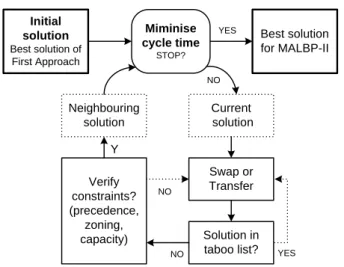
4.6 Addressing the problem of type II ... 87
4.6.1 First approach ... 88 4.6.2 Second approach... 89 4.7 Computational experience ... 90 4.7.1 Type I... 90 4.7.2 Type II ... 96 4.7.3 Additional goals... 98 4.8 Chapter conclusions... 99
5. Balancing U-shaped assembly lines ... 101
5.1 Chapter introduction ... 103
5.2 Characteristics of U-shaped assembly lines... 103
5.2.1 Literature review of approaches to solve the U-ALBP ... 105
5.3 Definition of the mixed-model U-ALBP ... 106
5.3.1 Problem assumptions and constraints... 108
5.3.2 Objective function ... 111
5.3.3 Complete mathematical programming model ... 114
5.4 U-ANTBAL: an ant colony optimisation based approach... 115
5.4.1 Use of parallel workstations ... 117
5.4.2 Numerical illustration ... 118
5.5 Computational experience ... 121
5.6 Chapter conclusions... 122
6. Balancing 2-sided assembly lines ... 123
6.1 Chapter introduction ... 125
iv
6.3.1 Problem assumptions and constraints ...128
6.3.2 Objective function ...131
6.3.3 Complete mathematical programming model ...132
6.4 2-ANTBAL: an ant colony optimisation based approach ...133
6.4.1 Building a balancing solution...135
6.4.1.1 Available tasks ...136
6.4.1.2 Selecting a task for assignment ...137
6.4.1.3 Assigning tasks to workstations ...139
6.4.2 Pheromone release strategy...140
6.4.3 Numerical example ...140
6.5 Computational experience ...142
6.6 Chapter conclusions...144
7. Real world applications ...147
7.1 Chapter introduction ...149
7.2 Case 1 – Combining heuristic procedures and simulation models for balancing a PC camera assembly line ...149
7.2.1 The PC camera assembly line ...150
7.2.2 Balancing the mixed-model assembly line...153
7.2.3 Development of the simulation models...158
7.2.4 Simulation experiment and results ...160
7.2.5 Conclusions ...164
7.3 Case 2 – Improving the performance of an assembly line by sequentially solving type I and type II problems ...164
7.3.1 Characteristics of the assembly line ...165
7.3.2 Two-step procedure for balancing the assembly line...167
7.3.3 Implementation of the proposed solutions ...169
7.3.4 Conclusions ...169
7.4 Case 3 – Increasing flexibility by turning a straight line into a U-shaped line ...170
v
7.4.4 Conclusions ... 174
7.5 Case 4 – Balancing a ‘n-sided’ assembly line ... 174
7.5.1 Characteristics of the assembly process ... 174
7.5.2 Adaptation of 2-ANTBAL to balance the assembly line ... 176
7.5.3 Addressing the assembly line planner’s preferences... 177
7.5.4 Conclusions ... 178 7.6 Chapter conclusions... 179 8. Conclusion ... 181 8.1 Final remarks ... 183 8.2 Future developments... 185 References ... 187 Appendix 1 Demonstration of the maximum and minimum values of functions Bb and Bw... 197
Appendix 2 Characteristics of the MALBP data sets... 201
Appendix 3 Computation of LBpmix for problems with maximum task processing time less or equal to 2C... 209
Appendix 4 Demonstration of the maximum and minimum values of functions B and bU U w B .... 215
Appendix 5 Computation of LBpmix for problems with maximum task processing time less or equal to 5C... 219
vi
Figure 2.1 Example of a precedence diagram ... 10
Figure 2.2 Types of assembly lines ... 11
Figure 2.3 An example of a combined precedence diagram ... 13
Figure 2.4 Binary integer programming model for the MALBP... 14
Figure 2.5 Assignment of tasks in straight and U-shaped assembly lines... 18
Figure 2.6 Configuration of a C-shaped assembly line ... 18
Figure 2.7 Illustration of the use of parallel workstations ... 20
Figure 3.1 Structure of a simulated annealing algorithm ... 26
Figure 3.2 Annealing schedule ... 27
Figure 3.3 Codification of a solution of a binary knapsack problem ... 31
Figure 3.4 Tournament selection ... 31
Figure 3.5 A crossover example ... 32
Figure 3.6 Standard encoding and the corresponding balancing solution ... 34
Figure 3.7 Example of crossover specific for standard encoding... 35
Figure 3.8 Two-point order crossover ... 36
Figure 3.9 Partially mapped crossover ... 36
Figure 3.10 Group encoding ... 37
Figure 3.11 Crossover in grouping genetic algorithms ... 37
Figure 3.12 The double bridge experiment... 41
Figure 4.1 Example of the variation of functions Bb and Bw for different scenarios ... 60
Figure 4.2 Mathematical programming model for the mixed-model ALBP with parallel workstations ... 62
Figure 4.3 The two-stage simulated annealing based procedure ... 63
Figure 4.4 Combined precedence diagram of the numerical example ... 68
Figure 4.5 Application of the SA based procedure to the numerical example ... 69
Figure 4.6 Global structure of the genetic algorithm based approach ... 70
Figure 4.7 Generation of two offspring through crossover ... 72
Figure 4.8 An application of the reassignment procedure ... 73
Figure 4.9 Variation of the fitness function in GA for two test problems... 75
vii
Figure 4.13 Outline of the modified version of ANTBAL ... 82
Figure 4.14 Procedure carried out by an ant to build a feasible solution... 84
Figure 4.15 Variation of the objective function in ANTBAL for two test problems ... 86
Figure 4.16 First approach to address MALBP-II ... 88
Figure 4.17 SA smoothing procedure for the MALBP-II... 89
Figure 4.18 An example of the variation of the workload balance functions... 99
Figure 5.1 Mixed-model production on a U-shaped assembly line ... 107
Figure 5.2 Possible combinations of models in a workstation in the same cycle. ... 112
Figure 5.3 Mathematical programming model for the U-MALBP... 115
Figure 5.4 Outline of U-ANTBAL ... 116
Figure 5.5 Building a balancing solution in U-ANTBAL ... 117
Figure 5.6 Straight and U-shaped line configurations for the numerical example ... 119
Figure 6.1 Configuration of a 2-sided assembly line ... 125
Figure 6.2 Interference in 2-sided assembly lines... 126
Figure 6.3 Mathematical programming model for the 2-MALBP... 134
Figure 6.4 Outline of 2-ANTBAL ... 135
Figure 6.5 Building a balancing solution for the 2-MALBP ... 136
Figure 6.6 Representation of a balancing solution for the 2-sided line ... 141
Figure 7.1 Exploded view of the PC camera ... 151
Figure 7.2 Combined precedence diagram for the three PC camera models... 152
Figure 7.3 Animation of the actual PC camera assembly system... 160
Figure 7.4 Simulation results for the average usage rate ... 162
Figure 7.5 Precedence diagrams of the five models ... 165
Figure 7.6 Combined precedence diagram for the five models ... 166
Figure 7.7 Two-step procedure for balancing the assembly line ... 168
Figure 7.8 Precedence diagram of one of the models ... 172
Figure 7.9 Assignment of operators to workstations for different production volumes 173 Figure 7.10 A wire harness assembly jig ... 175
Figure 7.11 Illustration of the wire harness assembly line ... 175
viii
Table 4.1 Processing times and average positional weights for the numerical example 68
Table 4.2 Main characteristics of the MALBP data set with typical task times ... 91
Table 4.3 Computational results for the MALBP-I data set... 92
Table 4.4 MALBP data set with random processing times ... 94
Table 4.5 Computational results for the MALBP-I data set with random times... 95
Table 4.6 Number of optimal solutions and maximum deviation obtained for Scholl’s data set... 96
Table 4.7 Computational results for the MALBP-II data set ... 98
Table 5.1 Task assignments and workload values for the two U-line solutions ... 120
Table 5.2 Computational results (number of operators) of U-ANTBAL for the two MALBP data sets ... 121
Table 6.1 Task processing times of models A and B ... 141
Table 6.2 Actions of the side-ants to build a balancing solution ... 142
Table 6.3 Results of the computational experience for 2-ANTBAL ... 144
Table 7.1 Task processing times ... 152
Table 7.2 Set of pairs of incompatible tasks ... 153
Table 7.3 Number of units to be produced for each demand level ... 153
Table 7.4 Demand values and cycle times for the different production scenarios... 154
Table 7.5 Initial solution for scenario 1 ... 155
Table 7.6 Final line configurations for the different demand scenarios... 156
Table 7.7 Comparison of theoretical and real cycle times ... 157
Table 7.8 Comparison of solutions with the lower bounds (LBpmix)... 157
Table 7.9 Simulation results for the average flow time ... 161
Table 7.10 Average usage rate and standard deviation ... 163
Table 7.11 Task processing times for the five models (t.u.) ... 166
Table 7.12 Results of the two-step procedure ... 168
Table 7.13 Comparison of performance measures between straight and U-shaped configurations... 174
Introduction
Contents
• Relevance of the problem
• Objective of the thesis
Assembly line balancing – new perspectives and procedures Ana Sofia Simaria
1.1
Relevance of the problem
The dynamics and intense competition in the current global marketplace together with the increased pace of technological change has led to shortening product life cycles and to a proliferation of product variety. Companies must be able to provide a higher degree of product customisation to fulfil the needs of the increasingly sophisticated customer demand (Su et al, 2005). Moreover, responsiveness in terms of short and reliable delivery lead times is demanded by a market where time is seen as a key driver. Mass customisation is a response to this phenomenon. It refers to the design, production, marketing and delivery of customised products on a mass basis. This means that customers can select, order and receive especially configured products, often selecting from a variety of product options, to meet their individual needs. On the other hand, customers are not willing to pay high premiums for these customised products compared to competing standard products in the market. They want both flexibility and productivity from their suppliers (Rudberg and Wikner, 2004).
As forecasting and planning become very complex, producing and storing all types of finished goods based on forecasts will lead to a high risk of stock out and obsolescence, while lead time often makes build-to-order impossible (Yang and Burns, 2003). Postponement arises as a strategy to contribute to the achievement of mass customisation. The concept of postponement is about delaying activities in the supply chain until real information about the market is available. The underlying logic is that the delay leads to the availability of more information and thus the risk and uncertainty of those activities can be reduced or even eliminated. In a postponement strategy uncertainty is seen as an opportunity instead of a problem (Yang et al, 2004, 2005).
Manufacturing postponement or delayed product differentiation is a type of postponement that seeks to delay the final formulation of a product until customer orders are received (Skipworth and Harrison, 2004). For example, in the automotive industry (high-volume vehicles), customers are allowed to choose their vehicle from a wide set of options. Customer involvement takes place only in the final assembly stage (Coronado et al, 2004).
Assembly line balancing – new perspectives and procedures Ana Sofia Simaria Delayed product differentiation involves shipping the products in a semi-finished state from the manufacturing facility to a downstream facility where final customisation occurs, normally as an assembly process. This strategy allows companies to standardise components and create a variety of products. Here, modularity plays an important role for a good performance of the system. It is an approach for efficiently organise complex products and processes by decomposing complex tasks into simpler portions so that they can be managed independently and yet operate together as a whole (Mikkola and Skjott-Larsen, 2004). Modularity consists in the breakdown of a complex part into simple and functionally independent components which are assembled to make customised parts. Although the number of parts in the modular design is larger than in the integral design, the total time of machining operations and manufacturing costs are more likely to decrease in the modular design. Nevertheless, modular designs increase the number of assembly operations and the assembly time and, hence, may require additional assembly stations in the system (He and Babayan, 2002).
Delayed product differentiation benefits the manufacturing process in two ways: it increases flexibility by enabling to commit the work-in-process to a particular end-product at a later time, and it decreases costs of complexity by reducing the variety of components and processes within the system (Nair, 2005).
The role of assembly lines has been changing through time. Assembly lines were firstly created to produce a low variety of products in high volumes. They allow low production costs, reduced cycle times and accurate quality levels. These are important advantages from which companies can benefit if they want to remain competitive. However, single-model assembly lines, designed to carry out a single homogenous product, are the least suited production system for high variety demand scenarios. As manufacturing is shifting from high-volume/low-mix production to high-mix/low-volume production, mixed-model assembly lines, in which a set of similar models of a product can be assembled simultaneously, are better suited to respond to the new market demands.
Instead of an inflexible production system, like they have been before, assembly lines are now an important piece of the supply chain, essential to support manufacturing postponement strategies. On one hand, assembly lines have the ideal structure to perform final product customisation tasks under a mass customisation concept. On the other hand,
Assembly line balancing – new perspectives and procedures Ana Sofia Simaria as they are labour intensive, assembly lines can be easily located geographically closer to the final customer marketplace.
The efficient design and operation of mixed-model assembly lines is, therefore, a crucial factor for the success of the supply chain in delivering customised products at low costs.
1.2
Objective of the thesis
The main objective of this thesis is to present a set of procedures to efficiently tackle different types of mixed-model assembly line balancing problems.
The proposed procedures based on the meta-heuristics, such as simulated annealing,
genetic algorithms and ant colony optimisation algorithms, are able to address some
particular features of the assembly process very common in real mixed-model assembly lines (e.g., use of parallel workstations, zoning constraints, task side constraints, U-shaped layouts) that most of the techniques covered in the current literature do not consider. This is a major contribution to scientific and industrial knowledge on the assembly line balancing subject.
Some of the procedures were applied to real assembly lines in order to test their efficiency to cope with real industrial settings, as they may differ significantly from theoretical problems. So, another goal of this thesis is to share the experience (successful applications and difficulties) of dealing with the conditions of real production systems.
1.3
Structure of the thesis
This thesis is divided in eight chapters. The present chapter briefly introduces the theme of the study, points out the relevance of the problem and presents the main objectives of the work.
The second chapter gives an overview of the assembly line balancing problem. It presents the main characteristics of assembly line systems and defines the assembly line balancing problem, emphasising the mixed-model perspective. Different types of assembly line configurations and particular features of the assembly process that may restrict the configuration of the lines are also presented.
Assembly line balancing – new perspectives and procedures Ana Sofia Simaria The third chapter is dedicated to review the available literature reporting meta-heuristic based approaches to tackle the assembly line balancing problem. It firstly describes the main characteristics of the selected meta-heuristics (simulated annealing, genetic algorithms and ant colony optimisation) and then presents a literature review of their applications to line balancing problems.
The fourth chapter presents the models and algorithms developed in this work for balancing mixed-model assembly lines with a linear configuration. A mathematical programming model was built to formally describe the problem and three heuristic procedures were developed to solve the problems. The procedures are based on well-known meta-heuristics, such as simulated annealing, genetic algorithms and ant colony optimization. A comparison between the performances of the three procedures, based on a set of computational experiments, is also provided.
In the fifth and sixth chapters mathematical programming models and heuristic procedures for balancing U-shaped assembly lines and 2-sided assembly lines, respectively, are presented. Conclusions about the heuristics’ performance are withdrawn, based on a set of computational experiments.
In the seventh chapter four industrial case studies are presented. They resulted from the analysis of real assembly lines and consequent application of the proposed heuristic procedures to improve the lines’ efficiency.
Finally, conclusions and directions for future research are pointed out in the eighth chapter.
2
2.
Overview of the mixed-model assembly
line balancing problem
Contents
• Chapter introduction
• Main characteristics of assembly line systems
• The mixed-model assembly line balancing problem
• Particular features of the assembly process
Assembly line balancing – new perspectives and procedures Ana Sofia Simaria
2.1
Chapter introduction
This chapter aims to provide an overview of the main features of production systems organised as assembly lines and to introduce the main concepts required to understand the mixed-model assembly line balancing problem – the object of the research presented in this work.
The chapter begins by introducing the main characteristics of assembly line systems, in order to point out the importance of mixed-model production, and the general mixed-model assembly line balancing problem is briefly described. Then, some particular features of the assembly line process that may be present in real assembly lines are described and the most common line performance measures are presented.
2.2
Main characteristics of assembly line systems
An assembly line is a set of sequential workstations connected by a material handling system, usually a conveyor belt. Manufacturing a product in an assembly line requires partitioning the total amount of work into a set of elementary operations called tasks. In each workstation a set of tasks is performed using a predefined assembly process, in which the following issues are defined:
the task processing time: the time required to perform each task;
a set of precedence constraints that, due to technological or organisational conditions, determine the sequence in which the tasks can be performed.
Figure 2.1 shows an example of a precedence diagram, in which the nodes represent tasks and the arcs express the precedence relationships between the tasks. For example, task 12 can only be performed after tasks 8 and 9 are completed (tasks 8 and 9 are direct
predecessors of task 12).
In a typical workstation the work is performed manually by human operators using simple tools or by semi-automated machines controlled by those operators. The time required to perform all tasks assigned to a workstation is termed workload.
Assembly line balancing – new perspectives and procedures Ana Sofia Simaria
Figure 2.1 – Example of a precedence diagram
In a paced assembly line each workstation has a predefined amount of time to complete all the tasks assigned to it: the cycle time. When this time is elapsed the sub-assembly must be moved to the next workstation and the workstation receives a new sub-assembly from the previous workstation. Thus, the cycle time determines the production rate of the assembly line. Since tasks are indivisible work elements, the cycle time cannot be less than the maximum task processing time (for assembly lines with no parallel workstations, as it will be explained in section 2.4.4). The difference between the cycle time and the workload is called workstation idle time. The sum of the idle times of all the workstations in the assembly line is the line idle time or total idle time.
In unpaced assembly lines there is no fixed time for a workstation to complete its tasks. All workstations operate at an individual speed so that sub-assemblies may have to wait before they can enter the next workstation and/or workstations may get idle waiting to receive a sub-assembly from the previous workstation. To avoid these difficulties, buffers between workstations are normally introduced in order to keep in-process inventories. The work developed in the present study only addresses paced assembly lines.
Considering the number of products to be assembled and the way they are processed, there are, basically, three types of assembly lines:
single-model assembly lines, in which a single homogenous product is continuously assembled in large quantities;
mixed-model assembly lines, in which a set of similar models of a product can be assembled simultaneously, in an arbitrarily intermixed sequence;
multi-model assembly lines, in which batches of similar models are assembled with intermediate setup operations.
Assembly line balancing – new perspectives and procedures Ana Sofia Simaria Figure 2.2 illustrates the different line types, where geometrical shapes symbolize the different models assembled on the line.
Figure 2.2 – Types of assembly lines
Single-model assembly lines are suitable for large-scale production, since they ensure very low production costs. High productivity is achieved by manufacturing a single product in very large quantities, using the principles of specialisation and division of work among operators. But long gone are the days when everyone could purchase a low priced car of ‘any colour as long as it was a black Model T Ford’.
The recent market trends show that there is a growing market demand for customised products, increasing the pressure for industries to diversify their production mix with more models and optional features being offered. Here it is evident the need for flexible systems, able to produce different versions of the same product without, however, increasing the costs excessively. This is the reason for companies to implement assembly line configurations, with specific measures being taken to make the system suitable for the production of different models. Assembly systems must still achieve high productivity, uniform quality and low assembly costs. Flexibility is also essential to cope with shorter product life cycles, low production volumes, changing demand patterns and a higher variety of product models and options.
In some cases multi-model lines are used: they can produce batches of different models with relatively low setup times. The line configuration is unique for each model so that tasks must be reassigned whenever the production changes from one model to another. When more flexibility is required the most suitable system is a mixed-model assembly line, in which setup is almost non-existent, allowing for the production of very small batches (even one-unit batches) in any sequence.
Assembly line balancing – new perspectives and procedures Ana Sofia Simaria According to Zhao et al (2004), there are two basic issues to address in mixed-model assembly lines: (i) at the ‘design’ level, the assignment of tasks to workstations in order to optimise a given ‘design measure’ and (ii) at the ‘operational’ level, the determination of the sequence in which the difference models are launched into the line, in order to optimise a given ‘operational performance measure’. The first is the balancing problem that must be addressed before building the line and the second is the sequencing problem that must be addressed everyday when implementing a production plan.
The present work addresses the balancing problem, which is defined in the following section.
2.3
The mixed-model assembly line balancing problem
The simple assembly line balancing problem (SALBP) was first mathematically formulated by Salveson (1955) and it consists in assigning a set of tasks, required to assemble a single homogenous product, to a set of workstations in order to minimise the number of workstations in the line or minimising the cycle time of the line (both these objectives are equivalent to minimise the idle time of the line). The assignment of tasks to workstations must ensure that the product demand is met and verify the following set of conditions (Shtub and Dar-El, 1990):
a task is indivisible and therefore must be totally performed in a single workstation; the sequence of the assigned tasks must respect the technological precedence
constraints;
all workstations have conditions to perform any task;
the task processing times are known and are independent of the workstation to which they are assigned;
the sum of the processing times of the tasks assigned to each workstation cannot exceed the cycle time, determined by the product’s demand.
The following characteristics are specific for the mixed-model assembly line balancing problem (MALBP):
a set of similar models is simultaneously assembled on the line; each model has a predefined demand over a planning horizon;
Assembly line balancing – new perspectives and procedures Ana Sofia Simaria the cycle time of the line is given by the ratio between the planning horizon and the
total demand of the different models;
each model has its own set of precedence relationships, but it is possible to combine all the relationships into only one precedence diagram – the combined precedence diagram, as exemplified in Figure 2.3;
the time required to perform a task may vary between the models;
workstations are flexible enough to perform their tasks on the different models.
Figure 2.3 – An example of a combined precedence diagram
According to the pursued goal, the MALBP can be classified into two different types, which are referred as dual problems (Scholl, 1999):
MALBP-I: minimises the number of workstations, for a given cycle time; MALBP-II: minimises the cycle time, for a given number of workstations.
In type I problems, the cycle time, and, consequently the production rate, has to be pre-specified, so it is more frequently used in the design of a new assembly line for which the demand can be easily forecasted. Type II problems deal with the maximisation of the production rate of an existing assembly line and are applied when, for example, changes in the assembly process or in the product range require the line to be redesigned. Both types of problems have the same mathematical formulation. The only difference is in what is given as input and what is the decision variable. While for type I the cycle time is given
Assembly line balancing – new perspectives and procedures Ana Sofia Simaria and the number of workstations is to be determined, for type II the opposite occurs, i.e., the number of workstations is given and the cycle time is to be determined.
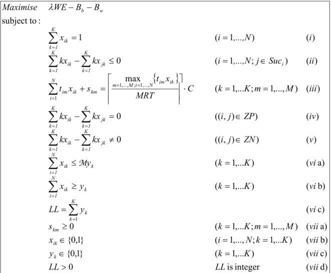
The MALBP can be formulated as a binary integer programming model, as presented in Figure 2.4, in which:
N is the number of tasks of the combined precedence diagram; M is the number of models assembled on the line;
Dm is the demand of model m over the planning horizon, P;
qm is the overall proportion of the number of units of model m being assembled,
given by
∑
= M p p m D D 1 / ; S is the number of workstations;
C is the line cycle time computed by
∑
= M m m D P 1 / ;
tim is the processing time of task i for model m;
Suci is the set of tasks that cannot be performed before task i is completed
(successors of task i), derived from the combined precedence diagram; ⎩ ⎨ ⎧ = otherwise 0, on workstati to assigned is task if 1, i k xik
{ }
0,1 1,..., ; 1,..., (5) ) 4 ( ,..., 1 ; ,..., 1 ) 3 ( , 0 ) 2 ( ,..., 1 1 : subject to ) 1 ( Minimise 1 1 1 1 1 1 1 S k N i x M m S k C x t Suc j N i kx kx N i x x t q C ik N i ik im i S k S k jk ik S k ik S k M m N i ik im m = = ∈ = = ≤ ∈ ∈ ≤ − = = ⎟⎟ ⎠ ⎞ ⎜⎜ ⎝ ⎛ −∑
∑
∑
∑
∑
∑ ∑
= = = = = = =Assembly line balancing – new perspectives and procedures Ana Sofia Simaria The objective function (1) minimises the weighted idle time of the assembly line, considering each model’s production share. This goal is equivalent to minimise the number of workstations for a given cycle time in MALBP-I and to minimise the cycle time for a given number of workstations in MALBP-II. The set of constraints (2) ensures that each task is assigned to only one workstation of the station interval and consequently tasks that are common to several models are performed on the same workstation. The precedence constraints are handled by the set of constraints (3) which guarantees that no successor of a task is assigned to an earlier station than that task. Constraints (4) are called capacity constraints and ensure that the workload of a workstation does not exceed the cycle time, regardless of the model being assembled. Finally the set of constraints (5) defines the domain of the decision variables.
The binary integer programming model becomes very complex even for small size problems, which makes it impossible to be solved to optimality in acceptable time. The problem is
NP
-hard (Scholl, 1999), which explains the interest of researchers in the development of heuristic procedures to address the problem.Although the minimisation of the idle time is the main goal of the MALBP, additional goals, like the workload balance between and within workstations, are also important to obtain good balancing solutions. Later in this work these goals will be described in detail and included in the proposed approaches.
2.4
Particular features of the assembly process
In order to better reflect the operating conditions of real assembly lines, some relevant issues of the assembly process need to be included when addressing an assembly line balancing problem. Scholl (1999) and Becker and Scholl (2006) present a comprehensive explanation on some particular features of the assembly process. Here, only a briefly description of these aspects is provided.
2.4.1
Variability of task processing times
The variability of task processing times depends on the nature of the tasks and operators. While for simple tasks the expected variance is very small, the processing time
Assembly line balancing – new perspectives and procedures Ana Sofia Simaria of complex and failure sensitive tasks may have significant variability, especially if performed by human operators, influenced by physical, psychological and social factors.
The use of deterministic values for the task processing times is justified when the expected variance is low. In most assembly lines using human workforce the number of tasks assigned to each operator is small and each task is usually very simple. Also, operators are especially trained to perform efficiently that small set of tasks. This way, the variability inherent to the human nature of the work is reduced by the simplicity of tasks and qualification of operators. The increased automation is also able to reduce the variability of task processing times, by using computer-controlled machines and robots able to work at constant speed.
If the tasks performed by human operators are long or complex, the variability of the task processing times should be considered when modelling the problem because the variance may significantly affect the system’s performance. In the case of automated lines, in which processing times are almost constant, there is a need to deal with the occurrence of machine breakdowns, by incorporating in the model a stochastic component of the task times reflecting the probability of machine breakdowns and the duration of repair processes.
When installing a new assembly line or introducing a new product in the line, the operators may have an adjustment period in which they take longer time to perform the tasks than after they are fully adapted. Dynamic task processing times may be used when learning effects allow systematic reductions or successive improvements of the production process.
2.4.2
Assignment constraints
Assignment constraints reduce the set of workstations to which tasks can be assigned. Several types of assignment constraints can be included in an assembly line balancing problem.
Zoning constraints force or forbid the assignment of different tasks to the same
workstation, being called positive or negative zoning constraints, respectively. Positive zoning constraints are normally related with the use of common equipment or tooling. For example, if two tasks need the same equipment or have similar processing conditions
Assembly line balancing – new perspectives and procedures Ana Sofia Simaria (temperature, pressure, operator qualification level, etc.) it is desirable that they are assigned to the same workstation. Negative zoning constraints are usually imposed by technological issues like, for example, when it is necessary to have a minimum time between the execution of the tasks or when it is not possible to perform them in the same workstation, for safety reasons.
Workstation related constraints are needed if special equipment is only available at a
determined workstation. Then the tasks that need that equipment must be assigned to that workstation.
In the case of large and heavy products (like cars, washing machines, etc.) the workpieces have a fixed position and cannot be turned. So, it may be necessary to perform tasks, for example, at both sides of the line. In this case a 2-sided line is used. It is, therefore, convenient to include position related constraints that group tasks according to the position in which they are performed.
When tasks require different levels of skills, depending on their complexity, operator
related constraints are needed to ensure that a sufficiently qualified operator is assigned
to a determined task. The qualification of an operator is determined by the most complex task assigned to its workstation. For ergonomic reasons, more monotonous tasks and more variable tasks should be combined in the same workstation in order to induce higher levels of job satisfaction and motivation.
2.4.3
Layout
In traditional or straight assembly lines, workstations are physically arranged along a linear conveyor belt and operators perform tasks on a continuous portion of the line. The implementation of just-in-time principles in industrial facilities made companies to switch from straight to U-shaped assembly lines. In a U-shaped line both ends of the line are closely together forming a ‘U’ and operators can move between the two legs of the line to perform combinations of tasks that would not be allowed in a straight line. It is an attractive alternative for assembly systems since operators become multi-skilled by executing tasks located at different parts of the assembly line. It improves visibility and communication between operators, which may facilitate problem solving. Also, a U-shaped line configuration allows for more possibilities on the assignment of tasks to
Assembly line balancing – new perspectives and procedures Ana Sofia Simaria workstations, so the number of workstations may be reduced, when compared with the number of workstations needed for a straight line. Figure 2.5 illustrates the differences between the assignment of tasks in straight and U-shaped assembly lines. A more detailed description of U-shaped assembly lines is provided in chapter 5.
Figure 2.5 – Assignment of tasks in straight and U-shaped assembly lines
Other assembly line layouts may be found in industrial facilities, like the C-shaped layout, illustrated in Figure 2.6 (Aase et al, 2004).
Assembly line balancing – new perspectives and procedures Ana Sofia Simaria
2.4.4
Parallelism
The implementation of parallel lines to assemble one or several products allows increasing flexibility and decreasing failure sensitivity of the production system. Parallel lines facilitate quick responses to product demand variations as the number of working lines can be easily changed. Also, the risk of production stoppage due to machine breakdowns is significantly reduced. Moreover, the cycle time can be increased, which brings additional advantages such as (i) better line balances, due to the higher number of possible task combinations and (ii) job enrichment, as the operators perform a larger number of different tasks.
The strategic problem of determining the optimal number of parallel line is of major importance as the duplication of lines involves increasing capital investment. However, when parallel lines are introduced, the number of tasks performed by each worker increases, the limit being one worker at each line performing all the tasks of the assembly process. This contradicts one of the main advantages of using assembly lines: the use of low skilled labour that can be easily trained (due to the strict division of labour). So, this aspect must be considered when installing parallel lines.
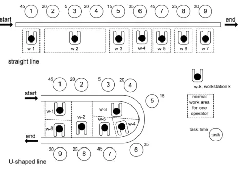
Even in single lines, parallelism can be implemented. When the production rate required to meet the demand is so high that the processing times of some of the tasks exceed cycle time, the implementation of parallel workstations is necessary to achieve the desired production rate. In parallel workstations, different workpieces are distributed among several operators who perform the same tasks. The local cycle time in these workstations is a multiple of the global cycle time, depending on the number of replicas installed. An example of the use of parallel workstations is shown in Figure 2.7. The longest task processing time of this example is 45, which limits the cycle time in the first configuration where no parallel workstations are used. With the use of parallel workstations it is possible to decrease the cycle time, for the same number of operators (seven), as it is shown in the second line configuration.
The use of parallel workstations is a common practice that allows a more flexible assignment of tasks and a reduction of the line cycle time. However, as for parallel lines, if the replication of workstations is not controlled, the advantage of the strict division of labour inherent to assembly lines can be lost.
Assembly line balancing – new perspectives and procedures Ana Sofia Simaria
1 2 3 4 5 6 7 8 9
w-1 w-2 w-5 w-6 w-7
45 20 5 20 15 35 45 25 30
start end
line without parallel workstations: cycle time =45
1 45 20 5 start end w-1 2 3 1 45 20 2 5 3 20 4 155 w-2 6 35 45 30 7 9 6 35 45 7 258 w-3 w-4 w-5
line with parallel workstations: cycle time =40 w-3 w-4
Figure 2.7 – Illustration of the use of parallel workstations
2.5
Assembly line performance measures
The implementation of an assembly line requires high capital investments, so it is very important that the line is designed and balanced to work as efficiently as possible. Also, re-balancing an existing assembly line is necessary when changes in the production process or demand structure occur. To assess the performance of the line, several criteria of technical and economical nature can be included in assembly line balancing problems.
According to Gosh and Gagnon (1989) the most widely used criteria of technical nature are related with the maximisation of the capacity utilisation which is measured by the line efficiency (the percentage of productive time in the line). Among them are (i) the minimisation of the number of workstations, for a given cycle time, (ii) the minimisation of cycle time, for a given number of workstations and (iii) the minimisation of the idle time of the line. Other capacity related criterion is the smoothing of workloads between the workstations, important to ensure similar workloads for all operators (see, for example, Merengo et al, 1999, Matanachai and Yano, 2001, Vilarinho and Simaria, 2002).
The economical nature criteria seek to minimise the total costs of the line, including long-term investment costs and short-term operating costs. Both installation and operation
Assembly line balancing – new perspectives and procedures Ana Sofia Simaria costs depend mainly on the cycle time and the number of workstations. As stated by Scholl (1999), the most important cost categories are (i) costs of machinery and tools, (ii) labour costs, (iii) materials costs, (iv) idle time costs, (v) penalties for not meeting the demand, (vi) incompletion costs, (vii) setup costs and (viii) inventory costs.
Several authors present multi-objective approaches. Shtub and Dar-El (1990) consider simultaneously (i) the minimisation of the line idle time and (ii) the minimisation of the number of parts at each workstation.
Malakooti (1991) includes (i) the number of workstations, (ii) the cycle time and (iii) the line operation costs, in his multi-criteria approach. In Malakooti (1994) the previous work is extended to include the size of buffers in the assembly line as another goal.
McMullen and Frazier (1998) use multi-objective criteria that comprise (i) the cost of labour and equipment, (ii) the workload balance between workstations and (iii) the probability of lateness.
Ponnambalam et al (2000) consider (i) the number of workstations, (ii) the workload balance between workstations and (iii) the assembly line efficiency as criteria to evaluate line balancing solutions.
Zhao et al (2004) aim to minimise the operational performance measure ‘total overload time’, i.e., the amount of time that exceeds the cycle time of the line, when considering mixed-model production. These authors state that the total overload appropriately reflects the relevant additional operating cost of the line, as when overload occurs the unfinished work has to be completed offline or the conveyor must be temporarily stopped to finish the tasks.
Besides capacity and cost related objectives, social goals may be important to fulfil, such as (i) job enrichment, avoiding the assignment of many monotonous tasks to an operator and (ii) job enlargement, increasing the number of tasks performed by an operator.
Although a wide variety of objectives may be included in line balancing approaches, the fact is that most of the objectives described in this section are basically influenced by the number of workstations and the cycle time of the line. Thus, this two goals can be considered the most important when balancing an assembly line.
3.
Meta-heuristics for assembly line
balancing: characterisation and review of
existing procedures
Contents
• Chapter introduction
• Simulated annealing algorithms
• Genetic algorithms
• Ant colony optimisation algorithms
• Taboo search algorithms
Assembly line balancing – new perspectives and procedures Ana Sofia Simaria
3.1 Chapter introduction
The assembly line balancing problem was firstly formulated by Salveson (1955) and, since then, numerous procedures have been developed to solve the problem. The literature on the subject is extensive and it focuses mainly on the simple version of the assembly line balancing problem. Comprehensive literature reviews on both exact and heuristic solution techniques for the different types of assembly line balancing problems are presented by Gosh and Gagnon (1989), Erel and Sarin (1998), Scholl (1999) and more recently by Becker and Scholl (2006) and Scholl and Becker (2006).
Although many optimising methods have been proposed, mainly branch-and-bound and dynamic programming procedures, their application is only possible for very restricted versions of the assembly line balancing problem, as the problem is
NP
-hard. To better reflect the characteristics of real world assembly lines, additional constraints must be included when solving the problem and this only increases its complexity. So, instead of exact procedures that find optimal solutions for simplified problems, heuristic procedures are used to find good solutions for much more complex problems. A large variety of heuristic approaches have been proposed in the literature. According to Scholl and Becker (2006), the development of constructive procedures, based on priority rules, to build one or more feasible solutions was presented in the literature until the mid nineties. In the last decade, the focus of researchers has been on improvement procedures using meta-heuristics like simulated annealing (Kirkpatrick et al, 1983), genetic algorithms (Holland, 1975, Goldberg, 1989), taboo search (Glover, 1989, 1990), and more recently, ant colony optimisation algorithms (Dorigo et al, 1996).Meta-heuristics are general search principles organised in a general search strategy used to solve combinatorial optimisation problems (Pirlot, 1996). They are able to search large regions of the solution’s space without being trapped in local optima, a major disadvantage of pure local search algorithms. As the research carried out for this work involves the application of meta-heuristics to mixed-model assembly line balancing problems, this chapter will focus on (i) the description of the main characteristics of the selected meta-heuristics (simulated annealing, genetic algorithms and ant colony optimisation
Assembly line balancing – new perspectives and procedures Ana Sofia Simaria
algorithms) and on (ii) the literature review of their application to assembly line balancing problems.
3.2 Simulated annealing algorithms
3.2.1 Overview
Simulated annealing (SA) is a randomised search technique that draws its inspiration from the physical annealing of solids. In this process, a solid is brought to its lowest energy state by first heating it to a very high temperature (usually the melting point temperature) and then cooling it at a very slow rate, to a very low temperature. When this heating and subsequent slow cooling occur, the particles within the solid rearrange themselves in such a way that the solid acquires some desired attribute, such as high strength or surface hardness.
The SA algorithm was introduced by Kirkpatrick et al (1983) to solve
NP
-hard combinatorial optimisation problems, by using the analogy with the simulation of the physical annealing of solids, in order to optimise the value of an objective function. Figure 3.1 presents the structure of a general SA algorithm.Assembly line balancing – new perspectives and procedures Ana Sofia Simaria
It starts from an initial solution to the problem, S0 and a control parameter, T, which is
set to an initial temperature value, T0. During the algorithm, the value of T is systematically
decreased according to an annealing schedule as shown in Figure 3.2. In this schedule the following issues are defined: (i) a temperature reduction function and (ii) the length of each temperature level, L, that determines the number of solutions generated at a certain temperature.
Figure 3.2 – Annealing schedule
At each temperature level, and as the temperature decreases, neighbouring solutions of the current solution are generated. A neighbouring solution, SV, is accepted, i.e., replaces
the current solution, if it is not worse than the current solution, S, (F(SV) ≤ F(S), where F is
the general objective function to minimise). If the neighbouring solution is worse than the current solution (F(SV) > F(S)), it still may be accepted with a certain probability, p=e-∆/T
where 100 ) ( ) ( ) ( × − = ∆ V V S F S F S F (3.1)
This probability of accepting inferior solutions allows the simulated annealing algorithm to escape from local minima.
S* is the best solution found by the algorithm.
The performance of the algorithm depends on the definition of the following annealing schedule parameters:
(i) The initial temperature, T0, should be high enough so that in the first iteration of
the algorithm the probability of accepting worst solutions is, at least, 80% (Kirkpatrick et al, 1983).
Assembly line balancing – new perspectives and procedures Ana Sofia Simaria
(ii) The most commonly used temperature reduction function is geometric: Ti=aiTi-1
(ai<1 and constant). Typically, 0.8≤ ai ≤ 0.99 (Eglese, 1990).
(iii) The length of each temperature level, L, determines the number of solutions generated at each temperature, T, and its value usually depends of the dimension of the problem.
(iv) The stopping criterion defines when the system has attained a desired energy level. Some of the most common stopping criteria are based on:
the total number of solutions generated;
the temperature at which the desired energy level is attained (freezing temperature);
the acceptance ratio (the ratio between the number of solutions accepted and the number of solutions generated).
Naturally, each of these control parameters must be refined according to the specific problem on hand. Two other important issues that need to be defined when adapting this general algorithm to a specific problem are the procedures to generate both the initial solution and the neighbouring solutions. These aspects will be addressed in the following section, in which a review of the application of SA procedures to the assembly line balancing problem is provided.
3.2.2 SA approaches for assembly line balancing
Heinrici (1994) proposes a SA procedure to solve the single-model assembly line balancing problem of type II, in which the objective is to minimise the cycle time for a given number of workstations. Suresh and Sahu (1994) solve the problem of type I and address variability by using stochastic task processing times. The SA approach presented by Erel et al (2001) aims at balancing U-shaped assembly lines. McMullen and Frazier (1998) present a multi-objective procedure to balance mixed-model assembly lines with stochastic task processing times and parallel workstations.
In the following sections a brief description of the application of simulated annealing to the assembly line balancing problem is provided, namely (i) the way the initial solution is obtained, (ii) the procedures to generate neighbouring solutions and (iii) the objective function used to evaluate the solutions and guide the search.
Assembly line balancing – new perspectives and procedures Ana Sofia Simaria
3.2.2.1 Initial solution
The precedence constraints of an assembly process determine the set of tasks available for assignment at a particular moment. The initial solution of a SA based procedure is typically obtained by a constructive heuristic, in which, from the set of available tasks, one task is selected according to a certain rule and assigned to the current workstation, as long as it does not exceed the workstation’s capacity. In the approach of Suresh and Sahu (1994) tasks are assigned according to their numerical order to build an initial feasible solution. The Ranked Positional Weight technique, originally developed by Helgeson and Birnie (1961), is the basis of the assignment of tasks to workstations in the initial solution of the procedure of Heinrici (1994). The assignment of tasks to workstations in the initial solution is done arbitrarily in the approach presented by McMullen and Frazier (1998).
Erel et al (2001) propose a different way of building the initial solution. First, each task is assigned to a different workstation and then the number of workstations is reduced by combining two adjacent workstations. When the workload of the combined workstation exceeds cycle time (leading to unfeasibility), the initial solution is complete and the subsequent steps of the SA procedure are initialised.
3.2.2.2 Neighbouring solutions
All the SA procedures mentioned in the previous section generate neighbouring solutions using two different movements:
(i) swapping two tasks in different workstations; (ii) transferring a task to another workstation.
The tasks and workstations are usually randomly selected and the resulting balancing solution must be feasible, regarding precedence and cycle time constraints.
3.2.2.3 Objective function
In the problem of type I the goal is to minimise the number of workstations for a given cycle time. But an objective function which only considers the number of workstations may not be effective, as there may exist several different balancing solutions with the same number of workstations. So, an important challenge is to determine an appropriate objective function that can efficiently guide the search through the solution space.
Assembly line balancing – new perspectives and procedures Ana Sofia Simaria
Depending on the nature of the problem or study, different objective functions are proposed to evaluate the balancing solutions and guide the SA procedure.
Dealing with stochastic task processing times, Suresh and Sahu (1994) use the probability of a workstation exceeding the cycle time and the balance of workloads between workstations (smoothness index) to compare their procedure with others available in the literature.
McMullen and Frazier (1998) in their multi-objective approach use the line design cost, the smoothness index and the probability of lateness to evaluate the solutions. They also build composite functions with combinations of these three objectives.
The SA procedure of Erel et al (2001) aims at achieving feasibility regarding cycle time constraints. The objective function used is the minimisation of the maximum station time, thus eliminating the unfeasibility caused by the workstation exceeding the cycle time.
Heinrici (1994) uses the minimisation of cycle time, as the addressed problem is of type II.
3.3 Genetic algorithms
3.3.1 Overview
Genetic algorithms (GA) are iterative search procedures, based on the biological process of natural selection and genetic inheritance, which maintain a population of a number of candidate members over many simulated generations. Hopefully the good characteristics of the members will be retained over the generations, maximising a determined fitness function.
GA do not operate directly on the solution space: solutions are coded in strings, over a finite alphabet, called chromosomes. An encoding is selected in a way that each solution in the search space is represented by one chromosome. Each chromosome is then decoded according to a user defined mapping function, enabling the computation of the corresponding fitness value, which reflects the quality of the solution represented by the chromosome. Figure 3.3 shows an example of representing a solution of the well known knapsack problem as a chromosome with binary codification. Each position in the
Assembly line balancing – new perspectives and procedures Ana Sofia Simaria
chromosome corresponds to an item, which takes the value 1 if it is selected and zero, otherwise. 0 0 1 1 0 1 0 1 1 0 0 1
Figure 3.3 – Codification of a solution of a binary knapsack problem
The most fit individuals (chromosomes) are selected to form a basis for subsequent generations, i.e., for reproduction. However, the selection is not deterministic. Each individual has a probability of being selected for reproduction that increases with its fitness. The selection scheme should provide a balance between population diversity and selective pressure in order to avoid premature convergence, allowing for an effective search. A very popular selection technique is called tournament and it aims to imitate mutual competition of individuals during casual meetings. It works the following way: two individuals are randomly selected from the population and the worst one is placed at the top of an empty list. The best individual returns to the population and the process is repeated until all individuals have been placed on the list. Then, starting from the top of the list, chromosomes are selected to undergo genetic operators. Figure 3.4 illustrates the tournament selection strategy (adapted from Falkenauer, 1998).
(i) select and evaluate the two individuals
list
(ii) put loser in list and winner back in the population
list
(iii) use the resulting order for crossover
list best
worst
Assembly line balancing – new perspectives and procedures Ana Sofia Simaria
The main genetic operator is the crossover, which has the role of combining pieces of information from different individuals in the population. The selected individuals (parents) are joined in pairs and combine their genetic material to produce two new individuals (offspring) as it is shown in Figure 3.5. The main objective of crossover is to transmit good characteristics from parents to offspring.
0 0 1 1 0 1 0 1 1 0 0 1 0 1 0 1 1 0 1 1 0 1 0 0 0 0 0 1 0 1 0 1 0 0 0 1 0 1 1 1 1 0 1 1 1 1 0 0
Figure 3.5 – A crossover example
Some individuals from the offspring population are randomly selected to undergo
mutation, i.e., small random changes are made in their genetic information. For example,
the mutation in a binary string is performed by changing the value of a randomly selected gene from 0 to 1 (or from 1 to 0). The use of mutation aims to ensure diversity among individuals, preventing premature convergence.
A replacement strategy is necessary to determine which individuals stay in the population and which are replaced by offspring. The members of the new generation can be (i) individuals from the current generation, (ii) offspring product of crossover or (iii) individuals who underwent mutation. The most common replacement approach is elitism, which allows the best chromosome in each generation to survive in the next generation, thus guaranteeing that the final population contains the best solution ever found. There are several approaches for the way the offspring replace their parents. Some favour the maintenance of the parents in the population while others always replace the parents by the offspring, even if they are worse than the parents. In either case, a random component is always present to avoid premature convergence to local optima.
In general, the main steps of a GA procedure are:
1. Generation of a random initial population of solutions in the form of chromosomes. 2. Evaluation of each individual in the population according to a pre-defined fitness
Assembly line balancing – new perspectives and procedures Ana Sofia Simaria
3. Selection of a set of individuals to undergo genetic operators. 4. Evaluation of the individuals created by the genetic operators. 5. Application of a replacement strategy to form the new generation.
6. If a satisfactory solution is achieved (or the stopping criteria are met, usually, a pre-defined number of generations), stop, otherwise go to step 3.
Several studies point out the effectiveness of GA in solving combinatorial optimisation problems, since they work with sets of solutions instead of only one solution at the time. Also they are flexible enough to include problem specific characteristics in the encoding scheme. The following section provides details of the application of GA to assembly line balancing problems and gives a review of the more relevant published approaches.
3.3.2 GA approaches for assembly line balancing
Evolutionary approaches have been widely applied to solve problems related with the design and organisation of manufacturing systems. In this section, solely the application of GA to the assembly line balancing problem (ALBP) is described. For other manufacturing problems the interested reader is referred to the reviews provided by Dimopoulos and Zalzala (2000) and Pierreval et al (2003).
The main challenge of the application of GA to the assembly line balancing problem is the development of good encoding schemes and genetic operators in order to attain feasible solutions. In the first part of this section, a review of the existing codification procedures and genetic operators is provided. A difficulty found in the application of GA to the assembly line balancing problem is related with the fitness function (Scholl and Becker, 2006). When addressing the assembly line balancing problem of type I, the objective function to minimise is the number of workstations. However, in a population, there might be several different solutions with the same number of workstations, so, the sole use of this performance measure as the fitness function may not be effective to guide the search. A review of the fitness functions proposed in the literature for the ALBP is presented, in the second part of this section. Finally, a glance of other features of the application of GA to ALBP is given in the last part of the section.