i
Smart Cities: Urban Green Infrastructures
Filipa Faria de Miranda Teixeira
Quantifying green infrastructures benefits and value
for cities sustainability
Project Work presented as partial requirement for obtaining
the Master’s degree in Information Management
ii
NOVA Information Management School
Instituto Superior de Estatística e Gestão de Informação
Universidade Nova de Lisboa
SMART CITIES: URBAN GREEN INFRASTRUCTURES
QUANTIFYING GREEN INFRASTRUCTURES BENEFITS AND VALUE
by
Filipa Faria de Miranda Teixeira
Project Work presented as partial requirement for obtaining the Master’s degree in Information Management, with a specialization in Knowledge Management and Business Intelligence
Co-Advisor: Miguel de Castro Simões Ferreira Neto, PhD Co-Advisor: Pedro Alexandre Reis Sarmento, PhD
iv
ABSTRACT
Populations have moved to cities and urban areas in recent years, resulting in their exponential growth. These migrations raise both traffic and resources consumption, leading to an increase of 𝐶𝑂2
emissions and contributing on a large scale to climate change. To extenuate the environmental issues adjacent to climate change, strengthening the number of urban trees is essential as they mitigate 𝐶𝑂2
emissions when incorporating carbon in their biomass. Understanding and measuring the extent of the role trees play as a mechanism for 𝐶𝑂2 storage introduces an interesting study that provides
information on urban green infrastructures planification. Additionally, attending the relation between carbon storage and carbon value, the trees represent a credit benefit for the cities. The incorporation of tree's species, age, and environment type on the previous analysis could also offer valid inputs to enhance the cities' decision making. With the present project, we will provide an interactive dashboard that complete and supports the current analysis.
KEYWORDS
Smart Cities; Urban Green Infrastructures; carbon storage; carbon value, tree species, urban trees, Viseu.
v
INDEX
1.
Introduction ... 1
2.
Literature Review ... 3
2.1.
Smart Cities ... 3
2.1.1.
Viseu City ... 3
2.2.
Urban Green Infrastructures ... 4
2.2.1.
Cities sustainability ... 5
2.2.2.
Green Infrastructure Economic Benefits ... 6
2.3.
Trees impact ... 7
2.3.1.
Carbon storage ... 8
2.3.2.
Allometric Equations ... 8
2.3.3.
Climatic changes ... 9
2.3.4.
Carbon Value ... 10
3.
Methodology ... 11
3.1.
Resource Data... 11
3.1.1.
Data Tools ... 11
3.2.
Cross-Industry Standard Process for Data Mining (CRISP-DM) ... 11
3.3.
Measure the carbon storage ... 12
4.
Data analysis ... 14
4.1.
Business Understanding ... 14
4.2.
Data Understanding ... 14
4.2.1.
Describe Data ... 14
4.2.2.
Explore data ... 14
4.3.
Data Preparation ... 15
4.3.1.
Rename variables ... 15
4.3.2.
Coherence Checking ... 16
4.3.3.
Handling missing values ... 17
4.3.4.
Handling outliers ... 18
4.4.
Modelling ... 18
4.5.
Data Visualization ... 21
5.
Results... 22
5.1.
Tree Species ... 22
5.1.1.
Variables Correlation ... 25
5.2.
Geographic analysis ... 30
vi
5.3.
Type ... 31
5.4.
Age and State... 33
5.5.
Reporting Dashboards ... 34
5.5.1.
Overview ... 34
5.5.2.
Species ... 34
5.5.3.
Details ... 35
5.5.4.
Geographic ... 36
5.5.5.
Variables Relation ... 37
5.5.6.
Information ... 38
6.
Conclusions ... 39
6.1.
Limitations and recommendations for future works ... 39
7.
Bibliography ... 41
8.
Appendix ... 1
8.1.
Exploring data ... 1
8.2.
Data coherence ... 2
8.3.
Handing missing values ... 3
8.4.
Data Modeler ... 4
8.5.
Number of trees and carbon storage by species ... 5
8.6.
Handling outliers ... 6
8.7.
Diameter at breast height e height equations impact ... 10
vii
LIST OF FIGURES
Figure 1: Trees relative frequency ... 22
Figure 2: Number of trees and carbon storage, as a percentage, by species ... 23
Figure 3: CO2 Value per Specie ... 24
Figure 4: Number of trees and CO2 relation ... 25
Figure 5: Diameter at breast height and CO2 Value relation ... 26
Figure 6: Height and CO2 Value relation ... 26
Figure 7: Carbon value in Viseu, by census tract ... 30
Figure 8: Number of trees by Type and Age. ... 32
Figure 9: CO2 value, by age ... 33
Figure 10: Age and state relation ... 33
Figure 11: Overview report, english version ... 34
Figure 12: Species report, english version ... 35
Figure 13:Details Report, english version ... 36
Figure 14: Geographic report, english version ... 37
Figure 15: Geographic report, english version ... 37
Figure 16: Information report, english version ... 38
Figure 17: Explorating Data Python Code ... 1
Figure 18: Part of Python Script results about Exploring Data ... 1
Figure 19: Data coherence ... 2
Figure 20: Handling missing values - python code I ... 3
Figure 21: Handling missing values - python code II ... 3
Figure 22: Data Modeler ... 4
Figure 23: Dbhcm distribution, by species family ... 6
viii
LIST OF TABLES
Table 1: Interval variables Statistics ... 14
Table 2: Absolute and relative frequency of the tree species present in the study area ... 15
Table 3: Rename variables correspondence. ... 16
Table 4: Coherence Checking rules ... 16
Table 5: Missing Values information ... 17
Table 6: Allometric Equations by Species Tree ... 20
Table 7: Diameter at breast height and Height impact, by species family ... 29
Table 8: Measures by locality ... 31
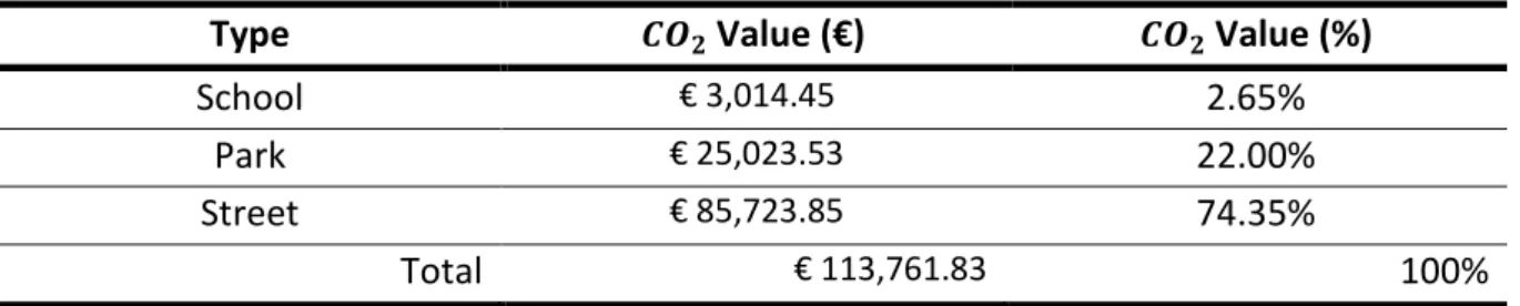
Table 9: 𝐶𝑂2 value and relative frequency by location type. ... 31
Table 10: 𝐷𝑏ℎ𝑐𝑚 detection of Outliers ... 7
Table 11: 𝐻𝑚 detection of Outliers ... 9
1
1. INTRODUCTION
Technology evolution happens not only at the companies but also in all society- including cities. There has been an increased recognition that more attention needs to be paid to this area. The new cities approach and strategies have based on technology and data, which contributes to develop and adopt the "smart cities" concept. Considering that nowadays cities have data it’s possible to have more information and produce knowledge... In orther words, with data and technology, we can understand the habitats, workers, and tourists. Posteriorly, the municipalities may plan, adapt, and manage its policies in a more sustainable way, making better and smarter, making better and more smart decisions. Cities work a crucial role in social and economic features worldwide and have a considerable impact on the environment. According to the United Nations, we predict that in 2030 more than 60% of the world population will live in cities (United Nations, 2018). Consequently, currently, most resources are consumed in cities worldwide, which contributes to economic development and at the same time to their poor environmental status. Cities account for 65% of global energy demand and 75% of global carbon dioxide emissions (Renewable Energy Policy Network for the 21st Century, 2019). However, when we increase the amounts of energy spent with transports and electricity, the lower the urban density, as proved by the fact that
𝐶𝑂
2 emissions per capita drop with the increase of urban areas density (Hammer, 2011).Towns are the centre of economic, people and the environment. The cities metabolism considers the goods input and the waste output with negative externalities, which means social and economic impact. Cities rely on too many external resources, and they are (and probably will always be) consumers of resource (Albino, Dangelico, & Berardi, 2015) . A recent and anthropocentric approach to urban sustainability, cities should respond to people's needs through sustainable solutions for social and economic aspects (Turcu, 2013).
Nowadays, we consider cities that discovery answers, opportunities and solutions for the citizen challenges and problems. Cities worldwide have started to look for solutions which enable transportation linkages, mixed land uses, and high-quality urban services with long-term positive effects on the economy (Albino, Dangelico, & Berardi, 2015). In that way, our mayors and cities are starting to worry about making and creating lively cities to respond to the population's needs. The big goal is offering more life quality and attract people. Therefore, the cities should be smart and give social, economic, environment and substantially policies for its residents, workers, or tourists.
Urban trees are outstanding sieves for urban pollutants and fine particulates. They can offer food, such as fruits. Spending time near trees improves physical and mental health by increasing energy level and speed of recovery while decreasing blood pressure and stress. Trees properly placed around buildings can reduce air conditioning needs by 30% and save energy used for heating by 20–50% (United Nations, 2016).
With the increase of the urban areas, trees could provide a pivotal measure to understand, and, respond to the urban trees impact on carbon storage in cities, as they stock carbon in their tissue though they grow. Trees absorb carbon dioxide and potentially harmful gasses, such as sulphur dioxide, carbon monoxide from the air and release oxygen. Also, they cool the air, land and water with shade and moisture, thus reduce the heat-island effect of our urban communities. The temperature in urban areas is often 9 degrees heater than in areas with substantial tree cover. Trees can help offset the build-up of carbon dioxide in the air and reduce the " greenhouse effect" (College of Agriculture & Life Sciences, 2019)
However, the ecological consequences of those National urban forest planting policies are still not clear. Besides, these kinds of ecological services are often primarily underestimated, and the potential of urban forest (UF) themselves to mitigate
𝐶𝑂
2 emission and climate change is far from being understood (Gaston, Ávila-Jiménez, Edmondson, & Jones, 2013). Hence, the precise and timely estimation of UF carbon storage is essential for cities to create strategic systems to improve urban𝐶𝑂
2 emissions mitigation (Ren & Zhai, 2019).2
Increasing flora cover in cities could be a pivotal approach to justify urban temperature excess. One way to measure the interactions between the urban environment and vegetation is to complete microclimate models that can simulate the effects of vegetation onto the urban microclimate, as well as the effects of urban environments onto vegetation. To provide reliable estimates, microclimate models need to be parameterised based on empirically obtained data.
At the same time, Environmental preoccupations are being more significant and are becoming an essential business for all of us. These issues range from global warming, temperature, 𝐶𝑂2
emissions,
acidification, melting and can even lead to extreme weather phenomena. Today these aspects are even more relevant, and 𝐶𝑂2emissions play a central role in the political agenda, due to the recognition that
𝐶𝑂
2emissions are the primary provider to climate change (United Nations , 2019). Attending to the
global and government preoccupation, the administration needs information to support its decisions. The goal of this thesis is to analyse the urban Trees’ power to measure carbon storage and Study trees’ impact on air quality in urban areas. We will combine the carbon storage with carbon produced and carbon monetary value of Viseu city which could represent a better approach to support the government decision making. For instance, at the beginning, we will address other points of view on the sustainable use of trees. Nevertheless, we found some challenges at the city data level.To support the decision making and our analysis, we will develop a dashboard using Power BI to better relate the additional variables like location, environment, age and status tree with its number, carbon storage and carbon monetary value. Our analysis will focus on three perspectives: species tree, geographic location and type age and status.
3
2. LITERATURE REVIEW
2.1. S
MARTC
ITIES"Smart City" concept does not have a standard definition. International Data Corporation (IDC) defines a "Smart City" as a city that has declared its intention to use information and communication technologies to transform modus operandi into one or more of the following areas: energy, environment, government, mobility, buildings, and services. Smart cities want to Increase their life quality, citizens and implement a sustainable economic growth. At the same time, the modernisation and information knowledge became crucial elements to discover the decisions making. It involves the use of digital and communication technologies and, as such, it strives towards high-quality resource management and service delivery (China Academy of Information and Communications Technology, EU-China Policy Dialogues Support Facility II, 2016). Considering other common concepts, like "digital city" or "city of the future", the difference is in "smart", which means data management and contains as one of its essential features project implementation from the "bottom-up" through the involvement of local communities (Crncevic, Tubic, & Bakic, 2017).
Currently, the leading Smart City focus on habitant/men. The technology evolution became part of the business, companies, and markets. In addition, data was spread all over society as well as the power to transform or convert them into knowledge. We can know what people bought, view, visited, liked or not. With this information, we could look at our cities and analyse social behaviour, to support decision making.
Urban territories contribute roughly seventy-five per cent on non-renewable energy source inferred 𝐶𝑂2 emanations, and numerous urban areas have instituted discharges relief plans. Assessment of the
viability of relief endeavours will require estimation of both the discharge rate and its change over the existence (Turnbull, et al., 2018). Cities strengthen population, business, industries, and energy output. Consequently, these are critical focal points to study improvement and emission 𝐶𝑂2 drivers'
opportunities.
2.1.1. Viseu City
The city is in Portugal Centre (40° 39'39.64 “N, 7° 54'34.96 “W). The municipality altitude is irregular, and it varies between 400 and 700 metres. The covered area is around 507.10 𝑘𝑚2 and divided into 25 parishes. Viseu is around 50 km east of Atlantic Ocean, encircled by mountains and it crossed by a rivers and streamlets network.
These characteristics make Viseu a city with a microclimate, with extreme temperatures: cold and wet winters and hot and dry summers. The average temperature is 19.2°, and the average precipitation is 1,198.5 mm. On the west side of the city, we can find Serra do Caramulo, which plays a significant role in climatic terms by reducing the impacts of the western air masses (while the Mondego River's basin makes the precipitation easier).
Viseu is also capital of the district with a population of 100 000 inhabitants. Two years ago, Viseu was in the top three of the healthiest councils, with greater security and quality of life (Cardoso, 2018) .
4 The municipality recognises resident's life quality as one of its priority goals, and it intends to become the best city to stay like to become the best city to stay, get a job, report, and invest (Cardoso, 2018). Viseu seeks to invest in tools that fix people that already live there, as well as attract new residents. In the environmental field, Cidade Jardim project emerged consisting on an exhaustive gathering of the city’s trees species. This project focus on a differentiated logic, for instance in the matter of pruning and the respective time of the year, including the analysis of late pruning. That will reduce the effect of pollens on people with allergies, or plan for replanting, removing some species to integrate others, explains Almeida Henriques (municipality mayor).
Additionally, the city has invested in improving the city's mobility infrastructures, with the creation of the new "Viseu Mobility Operations Center" and "Interface", the insertion of postcards, the implementation of the "Viseu Seguro" program" and implementing an environmental education project "Viseu Educating for Sustainable Mobility".
This town, by development all these initiatives, works to respond the goal of reducing more than 96,000 tons/year of
𝐶𝑂
2 by 2030, the promotion of energy and environmental sustainability, the promotion of the Information Society and Knowledge and promotion of active and healthy ageing in the county.Consequently, we believe that the present study may be an essential tool to support the municipality’s decision. Thus, we will make it possible to add more information to ongoing projects and contribute to the control of
𝐶𝑂
2 emissions per year, specifically (Ferreira, 2020).2.2. U
RBANG
REENI
NFRASTRUCTURESAfter the industrial revolution, the relationship between man and industry increased and became more prominent, causing a more significant influx of people in cities and a decline in agricultural and rural environments. Cities growth process was becoming faster and faster, marking the 20th century with the predominance of the city instead of the countryside.
During the 1920s and 1930s, modernism had invaded the cities. It had been segregated it in large functional areas. There, the focus had been on the economy with large commercial and industrial buildings and, at the same time, housing in big and high buildings as well. The green spaces appeared as multiple spaces for leisure. Since well-being in cities was associated with buildings, there was a contribution to less green spaces and environments.
Shortly after that, transports gave the impression that the city could disperse, as it allows for the intertwining of small towns. However, in practice, with the oil crisis in the 1970s, this concept became unsustainable. Urban expansion had an increasing impact, reaching levels of suburbanization (Mark Scott, 2016).
Then the new Urbanism was born, where compact and close city prevailed, as a result of a vibrant transport network. If, on one hand, rural spaces have been preserved, due to their abandonment, urban spaces have increasingly abdicated green spaces. At the same time, in the most notable towns, the transport network contributed to the reduction of car and the consolidation and greater efficiency in urban infrastructure (Mark Scott, 2016).
5 However, technological advances have introduced Geographic Information Systems in city planning as a tool for economic analysis and support for urban development. Furthermore, considering that society was becoming more aware of the impacts of the city’s environmental on human health and the benefits of green spaces for welfare municipalities were forced to focus on other values of natural areas beyond nature and biodiversity, namely those that would also respond to the needs of the populations.
The need to reverse urban development behaviours and the emergence of the sustainable development concept, in 1987, as a development to seek the satisfaction of the current generation’s needs, without compromising the ability for future generations to satisfy their own needs (United Nations, 1987), emphasizes the integration of the environmental component in planning. Thus, Green Infrastructure emerges as a territorial planning instrument, intending to defend the need for a more strategic and comprehensive approach to soil conservation.
Green Infrastructure concept has underlying notions that goes back to the beginning of Environmentalism, Nature Conservation, and the intervention of Landscape Architecture in 19th- century urbanism (Sussams, Sheate, & Eales, 2014). The Green Infrastructures is based on connections between green spaces and parks, in sequence to help populations and biodiversity preservation around the allocation of counterpoint corridors the habitat fragmentation (Samora-Arvela, Ferrão, Ferreira, Panagopoulos, & Vaz, 2017).
Accordingly, at a policy level, planning and the planning system needs to incorporate green infrastructures and an ecosystem approach to ensure that benefits are optimized in the long term, especially concerning global warming , biodiversity loss and climate change adaptation (CIWEM, 2010). We must plan and decide the infrastructures, in order to recognise the fundamental responsibility, it plays in the ecological and climate mindful growth of urban areas. Green infrastructures have an extensive range role with impact in quality life, and all the subsequent and related development from the beginning.
By taking care of the urban zones, the regards for the planet expands and green territories become more attractive, which increases the search for multifaceted, valued by both humans and the government. In that way, people have an interest in integrating dynamic and further action from cities, and the green infrastructures into the plan from development cities, becoming the green infrastructures plan a critical goal.
2.2.1. Cities sustainability
Urban Green Infrastructures can concentrate a big range of urban challenges, such as conserving biodiversity, adapting to climate change, supporting the green economy, and improving social cohesion. To capture this potential, local governments need to plan carefully and holistically.
According to Forest Research, there is a bright collection of proof which exhibits the remedial estimation of green space demonstrating that increasingly inactive types of use, or even merely access to perspectives on green space, can beneficially affect mental prosperity and individual capacity (Forest Research , 2010). We could provide opportunities for relaxation, exercise, and interaction with green areas, and when individuals are exposed to a green environment, stress levels decreased fast, compared with people who did not have this opportunity.
6 Maintainable reactions to economic and climate problems can help to solve social problems, such as being poverty and traffic congestion. Regardless, green spaces can also facilitate social interaction, integration, and the development of community cohesion (Forest Research , 2010). According to the Institute of Public Health reduced access to the natural environment can result in social isolation, obesity, and chronic stress. Consequently, access to green space is a significant predictor of increased physical activity (“active living”) and reduced risk of obesity (Heinze, 2011). Therefore, if Green infrastructures are related to parks, they play an essential role in helping physical activity in minority societies. it has been confirmed that people walking around parks shous a reduced stress rate across a broad spectrum of individuals (Hartig, Davis, Jamner, & Jamner, 2003).
Urban infrastructures and vegetation are typical for ecosystem assistance. They can decrease problems with flooding and generate positive effects on air quality (as a filter of polluted air). At the same time, improvements in air quality due to vegetation have a positive impact on physical health with apparent benefits as a decrease in respiratory illnesses (CemilBilgili & Gökyer, 2012). When people are in contact with green spaces, their stress levels decrease, which makes the correlation between nature and people more significant and with a greater influence on people’s lifestyle, work productivity and mental health.
The health benefits of regular walking have been widely reported, confirming that the benefits of this activity can contribute to reduce coronary heart disease and type 2 diabetes (Jones, M., & Coombes, 2009). Hence, green infrastructure can also support active travel, with incorporated walking and cycling, stimulating health.
Nevertheless, the links between green space and physical activity are not clear, and different studies have found contradictory results (Jones, M., & Coombes, 2009). Sometimes public spaces can attract criminal activities, such as drug dealers, nope – rapists. These criminal activities occur mainly because green spaces are often deserted at night, providing secluded and convenient venues for crime (Z., 2013). Nevertheless, a public study development in an inner-city found a correlation between lower crime rates and nearby vegetation (Kuo, 2001). That way, natural areas had the power to reduce crime and increase productivity, promote psychological wellbeing, decrease stress, and improve immunity. The effects in urban environments, cannot be over-stated and sometimes green space benefits are disproportionately distributed through the society. In other words, those who live in weak areas, the minority, the elderly, women, and people with disabilities, may not have access to the same levels of benefits. However, when the network has engaged with the arranging and usage of a green territory, its essence could be expanded as it assumes control over administration and responsibility for green territories in their region (Z., 2013).
2.2.2. Green Infrastructure Economic Benefits
Still, Green Infrastructure offers a high-quality environmental setting attracting new businesses which directly serve tourism, recreation, leisure, and health sectors (Forest Research , 2010). Frequently, people develop local activities where they live which contributes to urban green spaces becoming an input for relax and a local to usufruct these activities. However, the benefits are not only concentrated on the inhabitants of each region. Green infrastructure can attract and develop tourism, new local shops and get ideal exteriors for sports activities and a recreational variety.
7 Green infrastructure has also used as a valuable education resource. It has the potential to improve educational achievement, eventually helping to create a better qualified and more highly skilled workforce and bringing higher salaries and more valuable business investment into the region (Greater London Authority (GLA), 2008). With these green infrastructures in the cities there’s an increase in opportunities for educational events and jobs as forest warden, which consequently, creates more occasions to develop learning and employment.
The green infrastructure promotion and better respect can help decreasing management costs, like reduction in litter and other inappropriate practices. Green infrastructure provides a valuable, local resource for local schools and parents to use as a way of teaching children about sustainable development, conservation, environmental change, places, plants, animals, and natural and human-made processes (Okunlola, 2013). So, green infrastructure is a mechanism for sensitize and tell people about their environment.
Investment in Green Infrastructure can inspire and attract high-value industry, entrepreneurs, and skilled workers to a region through the creation of high quality, environmentally friendly living and working environments, value-adding to local economies (ECOTEC, 2008). It can offer leisure and recreation, opportunities creation and stimulate economic activity (forestry, parks, agriculture, and public services) with green infrastructure investment. These places are a way to attract and develop high-value industries, start-ups, businesspersons, and employees. Thereby, increasing the green infrastructures quality, the impact on the environment and society can also be positive so that it may add to economic performance.
When cities Increase their green economy, there are also linked prospects. They can create new jobs, limit the environmental impact of towns and cities, and reduce the costs of running them (Sustainable development Commission, 2010). Also, considering the minority, food acquiring makes up a significant part of a household’s income. So, the production that results from urban agriculture can be used for home consumption and as an effective way of supplementing income, thus contributing to poverty reduction (Z., 2013) . In this way, attending to subsistence, green infrastructures contribute to less expensive and capital cost, increasing the cost-effective approaches to manage runoff municipalities. The urban public park can help in increasing the property value the real estate market consistently demonstrate that many people are willing to pay a higher amount for a property located close to parks or open space areas than for homes that do not offer this facility (Okunlola, 2013). A park becomes one of a city’s innovations and attraction creation as a crucial advertising instrument to invite business, tourists, and conventions. Although the economic signal for the delivery of these profits is imperfect, these parks and green spaces can become profitable. The new green infrastructure development of current and new investments should be prioritized, particularly in areas that are significantly in need.
2.3. T
REES IMPACTDue to the growth of cities and harmful human activities, some species lost them habitats. At the same time, considering the environment and the species, this fact can become an opportunity to preserve some species. Nowadays, many cities contain sites of particular importance for conservation because they protect threatened species and habitats (CBO, 2012). So, many native fragments of vegetation
8 survived because of their geography, earth, and other characteristics. Increasing and planning cities according to the urban green infrastructures, could contribute to the biodiversity perseveration and control of some species behaviour.
Urban trees play a fundamental role in 𝐶𝑂2 storage as they act as a sink for 𝐶𝑂2 by fixing carbon during
photosynthesis and storing excess carbon as biomass (Nowak & Crane, 2002). That way, we need to understand the power and impact of the urban trees on carbon storage, as they collect carbon in their mass while growing.
Trees cool the air by throwing conceal and discharging water fume trees can channel fragile issues of particles - one of the most dangerous types of air contamination, produced from copying biomass and oil derivatives (The Nature Conservancy, 2016). On the other hand, to face the amount of carbon released into the atmosphere, derived from cities’ dimensions and human activities, the growth of trees has a greater importance and impact. Considering that the emissions caused by humans are higher than the number of trees saved, urban trees cannot be the only moderates. In parallel, trees also contribute with carbon to the atmosphere- when they die and rot. Consequently, by understanding how many carbons are stored by trees, we can become conscious about the amount of carbon that could be released when trees cease to exist.
Tree planting is becoming a strategy for city planners to mitigate heat and air pollution. Nevertheless, only trees can both renew and clean the air. Besides, trees and other green framework give a broad scope of co-benefits too—including territory for untamed life, stormwater control, entertainment openings, and beautification of open and private spaces in urban communities (The Nature Conservancy, 2016).
2.3.1. Carbon storage
In their biophysical process, trees trap and release 𝐶𝑂2 into the atmosphere. Throughout
photosynthesis, through leaves and by using the sun's energy, trees produce oxygen, vitamins, resins, and hormones necessary for their growth and health. It is based on the Carbohydrates retained throughout photosynthesis that trees grow, from where the respiration originates 𝐶𝑂2 storage by the
trees.
According to Aguaron and McPherson, the term "carbon dioxide storage" refers to the accumulation of woody biomass as trees grow over time. The similarity amidst the tree's biomass and the 𝐶𝑂2 stored
amount by it, in urban trees case, is proportional and it impacts on the tree density and management procedures (McPherson, Peper, & Van Doorn, 2016).
2.3.2. Allometric Equations
The allometric equations are the base to compute the carbon storage, using the diameter at breast height (𝐷𝑏ℎ), tree height, wood density, moisture content, site index and tree condition. Some of these parameters are correlated with climatic status and geographic area. Hence, some error is related to the use of regular densities and humidity contents in allometric formulas. We have two allometric biomass equations forms: volumetric and direct. Volumetric equations compute the overhead ground
9 volume of a tree using 𝐷𝑏ℎand tree height for the species. Linear equations produce beyond the ground dry weight of a tree using 𝐷𝑏ℎand tree height (McPherson E. A., 2012).
When we use allometric equation, we increase the uncertainty of our study. Though we have a lot of allometric equations developed for city trees, their precision needs to be more established when we apply it on an area with a challenging climate to define and to trees with significant size oscillations (McPherson E. A., 2012).
In city areas, we usually find many different tree species. Attending to E. Aguaron and, E.G. McPherson, we can find around 100 species in a city. Considering these tree diversity species and the allometric equation types scarcity for urban areas, most of the trees will be associated to a similar species or a family species equation. This fact increases our computation error associated with the equation choice (McPherson E. A., 2012).
2.3.3. Climatic changes
The Earth's climate has transformed during history. Few Scientists show an Earth-wide temperature boost propensity. This was seen since the mid-twentieth century to the human extension of the "nursery impact" — warming that outcomes when the climate traps heat transmitting from Earth toward space (NASA, 2018).
With climatic changes arises the Global warming concept, as a long-term rise in the average temperature of the Earth's climate system. It has been confirmed by direct temperature measurements and by various effects of warming, and its importance for climatic changes getting higher and higher (NASA, 2010). Some gases presented in the atmosphere are blocking the heat escaping. Long-lived gases stay "permanently" in the atmosphere "forcing" climate change (Stocker, et al.). With human activity, especially pollution and fossil fuels exploration, the temperature increases. Higher world temperature provides specific environmental problems, like melting of the ice caps, rising sea levels, acidification of the oceans, destruction of ecosystems, extinction of species, and, at least causes increasingly intense and frequent extreme weather phenomena (NASA, 2010).
On Earth, human activities are altering natural climatic. Over the last century, fossil fuels consumption of coal and oil has increased the intensity of atmospheric carbon dioxide (
𝐶𝑂
2). With the consumption of coal or oil, oxygen associates with carbon that is discharged into the air, shaping the𝐶𝑂
2. To a lesserdegree, the freeing from land for horticulture, industry, and other human exercises has expanded convergences of ozone-depleting substances (NASA, 2010). Considering the impact of the trees, they could play a critical role in the climatic changes combat.
The climate changes cause impacts on our entire society (business, families, and governments). To control it, we have built the social cost of carbon as a measure of the economic harm from those impacts.
10
2.3.4. Carbon Value
As we already mentioned, the carbon value corresponds to the social cost of carbon. It is expressed as the amount for the total damages from emitting one ton of carbon dioxide into the atmosphere, in euros (Environmental Defense fund, s.d.).
Attending to the Health Economic Assessment tool approach the carbon monetary value changes by each country and year. The price has in consideration the international facts, regional and country values.
When we compute the carbon monetary value of carbon, we calculate the hypothetical credits generated by the urban areas. This value, at the same time, stimulates climate-friendly securities, contributing to climate safety (Stempski, 2018).
11
3. METHODOLOGY
In this division, we introduce the methodology applied. First, we refer to the data source and data type used. Second, we present the data tools, techniques, and software used. Subsequently, we explain the data process adapted to respond to our problem since the input validation process data come out of the transformations and models required to final data set. Additionally, we describe the model methodology adopted, i.e., the formulas behind the request calculations.
3.1.
R
ESOURCED
ATAThe study is centred on the analysis and visualization of the secondary data obtained from the partnership between NOVA Cidade and Câmara Municipal de Viseu (Viseu City council). The data set was collected by the council government to develop studies and smart city projects to support decision-makers.
The project goal attends to quantify the carbon storage value and quantity using the most common tree species of Viseu.
3.1.1. Data Tools
This project mainly focuses on the Power BI tool. In the beginning, the dataset made available was in XML format. It was imported from Microsoft Excel to Microsoft Power BI.
In the initial part data processing and pre-processing and calculation of barometric equations, we will be using Python scripts inside Power BI. Later, when we create dashboards and make a visual data presentation, we will use Data Analysis Expressions (DAX).
3.2. C
ROSS-I
NDUSTRYS
TANDARDP
ROCESS FORD
ATAM
INING(CRISP-DM)
Cross-Industry Standard Process for Data Mining (CRISP-DM) is a six-stage model of the whole DM process. From beginning to end, that is exhaustively material across undertakings for a far-reaching display of data mining adventures. This methodology transforms business problems into data mining tasks, permitting holding projects independent of technology and applications (Wirth, 2000).
In the beginning, the CRISP-DM starts with a business understanding step. Here, the project goals are specified. This step determines a problem. At the “Data Understanding” phase, we need to describe the data, explore data, and verify data quality for the next steps in order to have the right data for our problem already defined. Afterwards, it follows the “Data Preparation“ phases, when we analyse data statistic, missing values, inconsistent data… the data focus on the business goal and adapts the values to that propose.
Additionally, the data sets can be “Modelling” to discover some parameter settings as desired, we built the data mining workflow for the nominated algorithms and to complete the data mining task on the
12 pre-processed data. In this phase, we adopt allometric equations to measure carbon storage. Surrounded by “Evaluation” the results reviewed attending to the core business objectives. Last, but not least, follows the “Deployment” step, where we implement or publish the project developed. We will use the CRISP-DM methodology to develop this project. First, we will clarify the project goals, understand, and prepare the data, with python scripts inside Power Bi. The modelling phases will require Allometric Equations, explained above. In the end, we respond to the evaluation and the deployment phases with Power Bi, building a dashboard to respond to the problem and to understand the results better.
3.3. M
EASURE THE CARBON STORAGEIn order to measure the carbon storage (𝐶𝑛) of each tree species, first, we started with the calculation
of the tress’ volume. To discover the volume value, we adapted the allometric equation for each tree, attending to its details and using the height and diameter of the tree Top (DAP_cm and Altura_m) variables. After that, we calculated the dry weight biomass, multiplying the weight density factor (specific value for each specie) (Neto & Sarmento, 2019) by the volume already calculated. Later, to calculate the total weight biomass and carbon and stored carbon dioxide, we multiplied the dry weight biomass (𝐷𝑤𝑏𝑛) by constant values. First, we computed the total dry weight biomass, the previous
dry weight biomass value plus the belowground biomass, with the product between 𝐷𝑤𝑏 and 1,28 (Husch, Beers, & Kershaw, 2003). At last, we converted the 𝑇𝑤𝑏 to 𝐷𝑤𝑐, multiplying by 1
2 (Leith,
1963). Ultimately, we estimated the stored carbon with the product between 44
12 and 𝐷𝑤𝑐 (McHale,
2009).
So, in short, with the purpose of measure the Viseu trees 𝐶𝑛, we calculated:
1. The trees volume by applying allometric equations according to the previous conditions: 𝑉𝑡𝑛= 𝑓(𝑑𝑖𝑎𝑚𝑒𝑡𝑒𝑟 𝑎𝑡 𝑏𝑟𝑒𝑎𝑠𝑡 ℎ𝑒𝑖𝑔ℎ𝑡, ℎ𝑒𝑖𝑔ℎ𝑡);
2. The trees dry weight biomass, i.e., the biomass of the tree visible part. For each tree was considered a certain dry weight density, according to the tree species, adopting the formula:
𝐷𝑤𝑏𝑛= 𝑉𝑡𝑛 × 𝐷𝑓𝑛 , 𝑤𝑖𝑡ℎ 𝐷𝑓𝑛= 𝑤𝑒𝑖𝑔ℎ𝑡 𝑑𝑒𝑛𝑠𝑖𝑡𝑦 𝑓𝑎𝑐𝑡𝑜𝑟;
3. Total dry weight biomass: part of the over and underground: 𝑇𝑤𝑏𝑛= 1.28 × 𝐷𝑤𝑏𝑛;
4. Dry weight carbon, that is, allows us to determine the carbon absorbed value for each tree:
𝐷𝑤𝑐𝑛= 𝑇𝑤𝑏𝑛 × 1 2 ;
5. Stored carbon: multiply the 𝐷𝑤𝑐 by 44
12:
𝐶𝑛= 44
13 After we calculated the stored carbon (𝐶𝑛), we considered relevant calculated carbon monetary value
associated. For each tree of Viseu, based on molecular weight, we compute the carbon monetary value with the product between the molecular weight of 𝐶𝑂2 -3.67- and carbon quantity. The 𝐶𝑂2 value for
each tree multiplied by the carbon projected social cost for Portugal in 2019:
12.74€
𝑡𝐶𝑂2 (World Bank Group,2019) (World Bank Group, 2019). The carbon cost social value of this tool is presented by country and year, based on global evidence, local averages, or country-specific values.
14
4. DATA ANALYSIS
4.1. B
USINESSU
NDERSTANDINGThe project aim is to study the potential of Viseu urban trees to measure stored carbon and carbon monetary value. For such, we had to estimate 𝑉𝑡, 𝐷𝑤𝑏, 𝑇𝑤𝑏, 𝐷𝑤𝑐, and 𝐶. At last, we provided a dashboard presentation to relate the variables and provide perspectives for analysis results.
4.2. D
ATAU
NDERSTANDING4.2.1. Describe Data
The dataset provides a total of 12,579 observations and 66 variables and corresponds to data collected between February 2017 and June 2018. In the beginning, we selected the most relevant variables for the analysis. We eliminated the ID variables and variables with higher missing data. To select which variables, we had to include in the analysis we built a Python script that provides a descriptive analysis, identifying the quantity observation and data type for a variable, [see Appendix 1].
4.2.2. Explore data
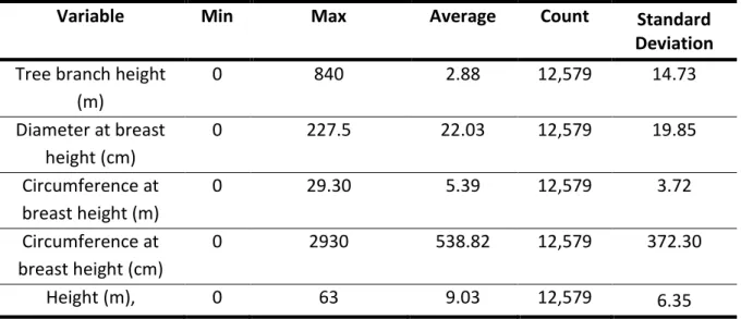
4.2.2.1. Interval Variables
After describing the data, we provided a statistic analysis of the interval variables- minimum, maximum, average, count and standard deviation for the variables, table 1.
Variable
Min
Max
Average
Count
Standard
Deviation
Tree branch height
(m)
0
840
2.88
12,579
14.73
Diameter at breast
height (cm)
0
227.5
22.03
12,579
19.85
Circumference at
breast height (m)
0
29.30
5.39
12,579
3.72
Circumference at
breast height (cm)
0
2930
538.82
12,579
372.30
Height (m),
0
63
9.03
12,579
6.35
15
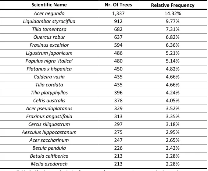
4.2.2.2. Categorical Variables
For the categorical variables, we calculated the number of individuals and their relative proportions for each category. With the presented analysis, we observed that the dataset provides data about a lot of scientific species. So, we focused our study on 20 most representative species, table 2:
Scientific Name
Nr. Of Trees
Relative Frequency
Acer negundo
1,337
14.32%
Liquidambar styraciflua
912
9.77%
Tilia tomentosa
682
7.31%
Quercus robur
637
6.82%
Fraxinus excelsior
594
6.36%
Ligustrum japonicum
486
5.21%
Populus nigra 'italica'
480
5.14%
Platanus x hispanica
450
4.82%
Caldeira vazia
435
4.66%
Tilia cordata
435
4.66%
Tilia platyphyllos
396
4.24%
Celtis australis
378
4.05%
Acer pseudoplatanus
329
3.52%
Fraxinus angustifolia
313
3.35%
Cercis siliquastrum
297
3.18%
Aesculus hippocastanum
275
2.95%
Acer saccharinum
247
2.65%
Betula pendula
226
2.42%
Betula celtiberica
213
2.28%
Melia azedarach
213
2.28%
Table 2: Absolute and relative frequency of the tree species present in the study area
4.3. D
ATAP
REPARATIONOn the Data Preparation, we started by renaming some variables, attending to the names provided by the methodology adopted. After that, we checked the incoherencies in numerical variables, handling missing values.
4.3.1. Rename variables
16
Variable
Variable source name
New name
Tree branch height (m)
Alt_ramo_m
ℎ𝑏𝑚Diameter at breast height
(cm)
DAP_cm
𝑑𝑏ℎ𝑐𝑚Circumference at breast
height (m)
d_copa_m
𝑑𝑐𝑚Circumference at breast
height (cm)
d_copa_cm
𝑑𝑐𝑐𝑚Height (m),
Altura_m
ℎ𝑚Table 3: Rename variables correspondence.
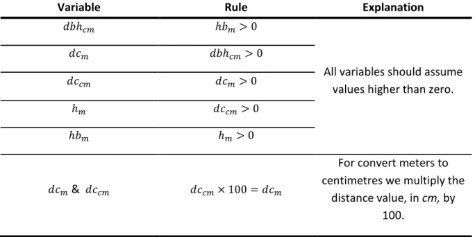
4.3.2. Coherence Checking
The coherence checking helped to verify if the analysis dataset had consistent data. Some rules were checked, to see if there was any incoherence data. Furthermore, in the beginning, we checked if the dataset had duplicates, although not applicable. For that, conditions were created to delete the incoherence data, table 4:
Variable
Rule
Explanation
𝑑𝑏ℎ𝑐𝑚 ℎ𝑏𝑚 > 0
All variables should assume
values higher than zero.
𝑑𝑐𝑚 𝑑𝑏ℎ𝑐𝑚 > 0
𝑑𝑐𝑐𝑚 𝑑𝑐𝑚 > 0
ℎ𝑚 𝑑𝑐𝑐𝑚 > 0
ℎ𝑏𝑚 ℎ𝑚> 0
𝑑𝑐𝑚
&
𝑑𝑐𝑐𝑚 𝑑𝑐𝑐𝑚× 100 = 𝑑𝑐𝑚For convert meters to
centimetres we multiply the
distance value, in cm, by
100.
Table 4: Coherence Checking rules
Additionally, we removed the duplicates and error values, in total, we deleted 435 observations, corresponding to a proximally 3% of the original data set. The summary of this python script can be seen in the [see Appendix 2].
17
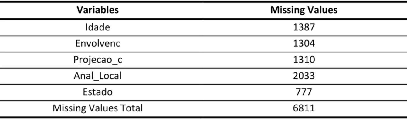
4.3.3. Handling missing values
The variables with missing values are categorical variables. So, to handle missing values, us applied an Extra-Trees Regressor and we filled the missing values with predictive values. This technique implements a meta estimator that fits randomized decision trees on various sub-samples of the dataset. It uses averages to adjust the predictive precision and control over-fitting.
The decision trees split the data into sets of mutually restricted records. When we used more than one decision tree, we built a decision forest that identifies data with even better similarity (among the records) and higher correlations (among the attributes). We used this technique because sometimes, a dataset probably has records within a section that have higher similarity and attribute correlations comparing to the similarity and correlations of the whole data set (Rahman & Zahidul, 2013). Additionally, when we use the data partition for the replacement, we can give better accuracy imputation.
With Extra-Trees Regressor, a random dataset partition is applied, however, it extracted the best random thresholds. At the same time, these are randomly selected the same as the splitting rule. It permits reducing the model variance, increasing the bias.
Once we had categorical variables, we had to transform it in numerical variable. In that way, we created an index that corresponds each categorical variable to a number. Attending to the variables used, we found a total of 6 variables with missing data, table 5:
Variables
Missing Values
Idade
1387
Envolvenc
1304
Projecao_c
1310
Anal_Local
2033
Estado
777
Missing Values Total
6811
Table 5: Missing Values information
After that we built a python code, [see Appendix 3], to apply the predictive decision tree imputation. Once we are using categorical variables this imputation it could be influential in correlation between the variables. With the python code our dataset had numerical variables rather than categorical and text variables. So, to impute the values in really dataset, we merged by OBJECTID variable the data set before and after imputation.
At this point we had a new dataset like an outer join of the previous table and the new table-without the missing values. First, we built support tables with index and respective descriptions and after, we connected the additional tables with the bases. So, inside Power BI we built the correspondence between the new numerical values, that we produced applying the decision tree technique, and its description, presented in additional tables.
18 Additionally, we found missing values on variables freguesia and localidade (parish and zone). Heretofore, we have the street, latitude, and longitude of each tree, manually we substituted the missing values for the correct value.
4.3.4. Handling outliers
The current study focusses principally on descriptive statistics analysis. Attending to that, we will handle the outliers just for the study part of dimension tree variables and it is the correlation with 𝐶𝑂2.
4.4. M
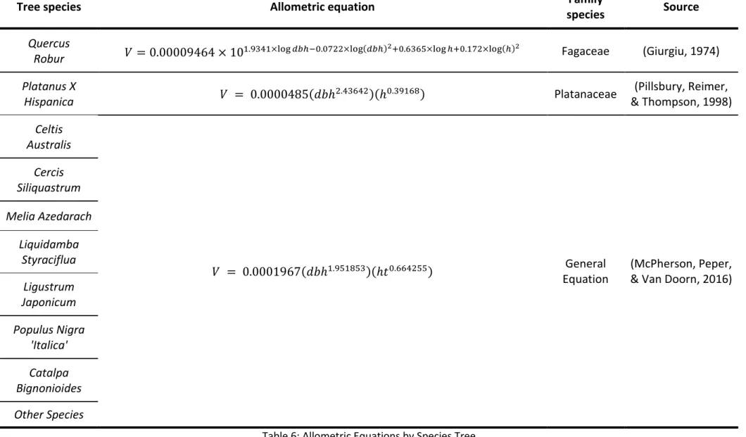
ODELLINGTo compute the new variables (volume, total dry weight biomass, total dry weight biomass of carbon, dry weight biomass, and carbon storage), we used allometric equations that we recovered from the GlobAllomTree database (Henry, et al., 2013) presented on the website (http://globallometree.org/). Since not all trees have an allometric equation associated, but only one similar tree species, which in turn has an allometric equation, we grouped the species tree in family species. When there were no similar species of the equivalent genus, we applied a general equation for broadleaf trees (Mcpherson & Doorn, 2016). In our equations, we considered the 𝐷𝑏ℎ𝑐𝑚and the h in meters, table 6.
19
Tree species
Allometric equation
Family
species
Source
Acer
Negundo
𝑉 = 0.012668 + 0.0000737 × 𝑑𝑏ℎ
2× h
0.75Aceraceae
(Centre for Ecology
& Hydrology, 2005)
Acer
Pseudoplatanus
Acer Sacharinum
Tilia
Cordata
𝑉 = 0.00004124 ×
10
(1.9302×log 𝑑𝑏ℎ)+(0.0209×((log(dbh))2))+(0.129×log ℎ)−(0.1903×((log ℎ)2))Malvaceae
(Giurgiu, 1974)
Tilia
Platyphyllos
Tilia
Tomentosa
Fraxinus
Excelsior
𝑉
= 0.00030648
∗ 10
1.2676∗𝑙𝑜𝑔10((𝑑𝑏ℎ))+0.3102∗𝑙𝑜𝑔10((𝑑𝑏ℎ))2+0.4929∗𝑙𝑜𝑔10((ℎ))+0.0962∗𝑙𝑜𝑔10((ℎ))2Oleaceae
(Giurgiu, 1974)
Fraxinus
Angustifolia
Betula
Pendula
𝑉 = 8.141 × 10
−5× 10
2.248×𝑙𝑜𝑔(dbh)−0.2062×𝑙𝑜𝑔(dbh)2+0.1946𝑙𝑜𝑔(h)+0.4147𝑙𝑜𝑔(ℎ)2Betulaceae
(Giurgiu, 1974)
Betula
Celtiberica
20
Tree species
Allometric equation
Family
species
Source
Quercus
Robur
𝑉 = 0.00009464 × 10
1.9341×log 𝑑𝑏ℎ−0.0722×log(𝑑𝑏ℎ)2+0.6365×log ℎ+0.172×log(ℎ)2
Fagaceae
(Giurgiu, 1974)
Platanus X
Hispanica
𝑉 = 0.0000485(𝑑𝑏ℎ
2.43642)(ℎ
0.39168)
Platanaceae
(Pillsbury, Reimer,
& Thompson, 1998)
Celtis
Australis
𝑉 = 0.0001967(𝑑𝑏ℎ
1.951853)(ℎ𝑡
0.664255)
General
Equation
(McPherson, Peper,
& Van Doorn, 2016)
Cercis
Siliquastrum
Melia Azedarach
Liquidamba
Styraciflua
Ligustrum
Japonicum
Populus Nigra
'Italica'
Catalpa
Bignonioides
Other Species
21 Attending to higher quantity of data and species trees, we considered at least 75% and we found an allometric equation or apply the general equation if it is the case. The other 25% of the trees assume the general equation too.
After that, we computed the additional variables (𝑑𝑤𝑏, 𝑇𝑤𝑏, 𝐷𝑤𝑐, 𝐶𝑎𝑟𝑏𝑜𝑛 𝑆𝑡𝑜𝑟𝑎𝑔𝑒, 𝐶𝑚𝑣 and 𝐶𝑂 2𝑉𝑎𝑙𝑢𝑒) attending to the formulas explained before. These calculations were made directly on
Power Bi data visualization tool.
In the same way the dataset provides variables such parishes, zone, age, place planted (i.e., if the tree is in a school, street, or park area), projection, state and local analysis, beyond the geographical coordinates, we could combine it with previous values calculated and the species trees. The data model was developed on Microsoft Power BI [see Appendix 4].
4.5. D
ATAV
ISUALIZATIONThe motivation for the presented study was to get insights about the places, where trees are located, relating it with tree features and analysing their relationship with carbon storage and value. To fundament the study and give support to community decision-makers for trees plantation planning measures, we developed a reporting dashboard to respond to the following questions:
▪ In which zones of Viseu were higher values of carbon storage?
▪ What is the age of the trees? And how much 𝐶𝑂
2is stored in those areas?
▪ Are the trees situated at schools, parks, or street? How many carbons can they
store?
22
5. RESULTS
Here, we provide some experimental evaluation of the new technique. The approach adopted to analyse the study results include four perspectives: tree species, geographic analysis, age and state and type analysis. In each perspective we have in consideration the number of trees, carbon storage and 𝐶𝑂2 value.
5.1. T
REES
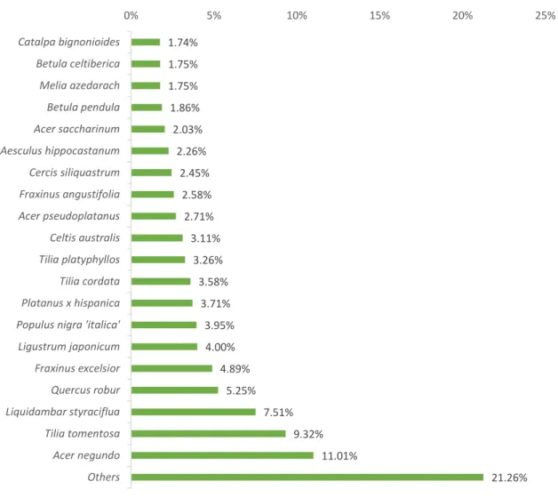
PECIESThe most represented tree species was Acer Negundo, with 11.01% of individuals, followed by Tilia
Tomentosa and Liquidambar styraciflua with 9.32%. and 7.51%, respectively. The presented dataset
has a higher number of tree species and we cannot find a dominant species. Additionally, when we agglomerate the trees in Others, we create a most representative category species. The trees did not have missing values in its species and dimensions data. In Figure 1 is presented the relative frequency for each tree species (Nh) from the total of 12,144 trees – after data preparation.
Figure 1: Trees relative frequency
The total carbon amount stored by the 12,144 trees of Viseu was 8,921Kg, with a higher contribution of the Tilia tomentosa, 2,572Kg and Platanus x hispanica, 2,548Kg. In the same way of the previous
1.74% 1.75% 1.75% 1.86% 2.03% 2.26% 2.45% 2.58% 2.71% 3.11% 3.26% 3.58% 3.71% 3.95% 4.00% 4.89% 5.25% 7.51% 9.32% 11.01% 21.26% 0% 5% 10% 15% 20% 25% Catalpa bignonioides Betula celtiberica Melia azedarach Betula pendula Acer saccharinum Aesculus hippocastanum Cercis siliquastrum Fraxinus angustifolia Acer pseudoplatanus Celtis australis Tilia platyphyllos Tilia cordata Platanus x hispanica Populus nigra 'italica' Ligustrum japonicum Fraxinus excelsior Quercus robur Liquidambar styraciflua Tilia tomentosa Acer negundo Others
23 analysis the Other Species represent a higher value, with 3,266Kg carbon stored, [see Appendix 5]. Therefore, we can observe that the most representative defined species do not represent the tree that absorbs more carbon, Figure 2.
Figure 2: Number of trees and carbon storage, as a percentage, by species
At the same time, according to Figure 2 we can observe species that have higher 𝐶𝑛 Value comparing
to its number of trees. For example, Melia azedarach species with less than ½ of representative of
Quercus robur, 213 and 637 trees respectively, have more than a double of the 𝐶𝑛 Value: 135.63Kg
and 56.99Kg [see ppendix 5].
3.3% 3.6% 1.9% 2.6% 2.0% 1.8% 5.3% 2.5% 4.9% 2.7% 4.0% 1.8% 1.7% 2.3% 7.5% 3.1% 11.0% 4.0% 3.7% 9.3% 25.0% 0.1% 0.1% 0.4% 0.5% 0.5% 0.5% 0.6% 0.8% 1.0% 1.1% 1.2% 1.5% 1.6% 2.6% 3.3% 3.4% 5.7% 9.8% 28.6% 28.8% 36.6% Tilia Platyphyllos Tilia Cordata Betula Pendula Fraxinus Angustifolia Acer Saccharinum Betula Celtiberica Quercus Robur Cercis Siliquastrum Fraxinus Excelsior Acer Pseudoplatanus Ligustrum Japonicum Melia Azedarach Catalpa Bignonioides Aesculus Hippocastanum Liquidambar Styraciflua Celtis Australis Acer Negundo Populus Nigra 'Italica' Platanus X Hispanica Tilia Tomentosa Others
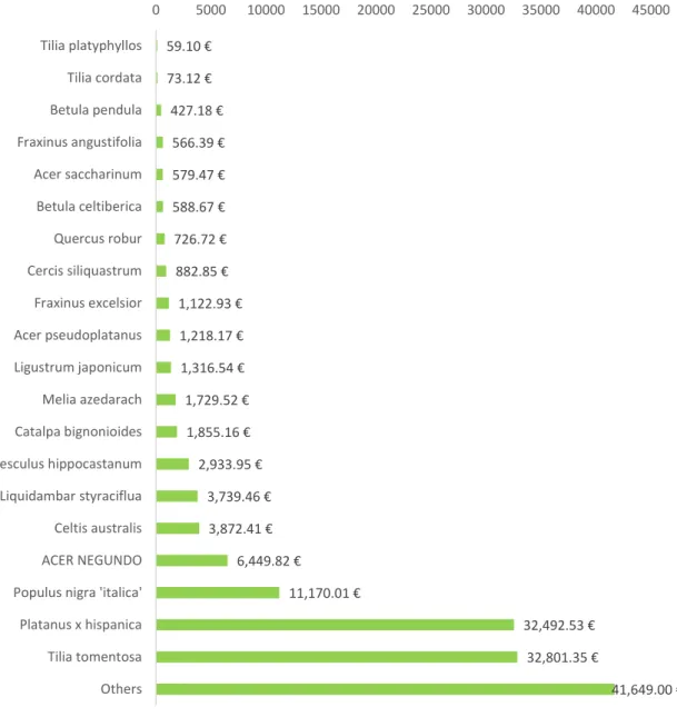
24 According to the 𝐶𝑂2 value, as expected, we were able to detect the same behaviour by species.
Agreeing to Figure 3, the species Tilia tomentosa is the one that gives the most credit for carbon dioxide to the city 32,801€, followed by Platanus x Hispanic 32,493€ and Populus nigra 'italica' 11,170€. For their part, the species included in the Others offer the largest credit € 41,649€ The species with the lowest stored carbon dioxide are those that, likewise, contribute less credit to Viseu.
Figure 3: 𝐶𝑂2 Value per Specie
We found significant positive effect on carbon storage for tree species because the total carbon amount that was stored by species, like Tilia Tomentosa, Platanus x hispanica or populus nigra ‘italica’ are higher than acer negundo or liquidambar. This second species group represents more trees quantity when compared with first group mentioned.
At the same time, we found no significant consist effect for trees amount. So, the figure 4 shows a positive relation between the 𝐶𝑂2 Value and number of trees. Although, the points scattered across
the graph and the lower R2 indicate the security does not generally follow a linear behaviour.
59.10 € 73.12 € 427.18 € 566.39 € 579.47 € 588.67 € 726.72 € 882.85 € 1,122.93 € 1,218.17 € 1,316.54 € 1,729.52 € 1,855.16 € 2,933.95 € 3,739.46 € 3,872.41 € 6,449.82 € 11,170.01 € 32,492.53 € 32,801.35 € 41,649.00 € 0 5000 10000 15000 20000 25000 30000 35000 40000 45000 Tilia platyphyllos Tilia cordata Betula pendula Fraxinus angustifolia Acer saccharinum Betula celtiberica Quercus robur Cercis siliquastrum Fraxinus excelsior Acer pseudoplatanus Ligustrum japonicum Melia azedarach Catalpa bignonioides Aesculus hippocastanum Liquidambar styraciflua Celtis australis ACER NEGUNDO Populus nigra 'italica' Platanus x hispanica Tilia tomentosa Others
25 Figure 4: Number of trees and 𝐶𝑂2 relation
We applied different allometric equation to compute de trees volume so, we considered that finding common behaviour between the variables was unnatural. The higher values in dimension data could explain the higher 𝐶𝑂2 Value, however the same rationale could be associated to species like Platanus x hispanica, it has the higher tree branch, 𝑑𝑏ℎ𝑐𝑚, ℎ𝑚 mean values.
5.1.1. Variables Correlation
The main goal before the analysis was done was to impute the outliers to have a segmentation with more reliable results. If the original outlier’s value were included in this analysis, the results would change very significantly. As such, a boxplot for both variables, diameter at breast height e height, was used, allowing to see its distribution without doing any damage to the representativeness of the population [see appendix 6].
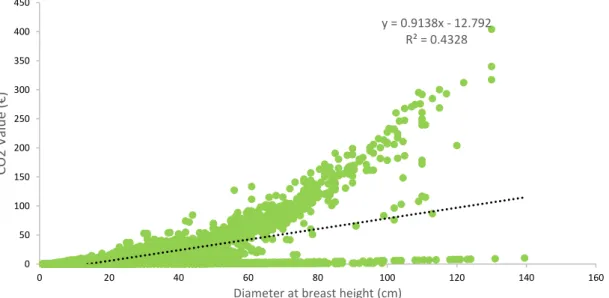
Consequently, per species, despite the positive relationship between the number of trees and 𝐶𝑂2
Value, we could not find an evident relation between them, figure 5 and figure 6. If we had considered a linear relation between them, we would get a R square lower than 0.5 in both cases.
R² = 0.3823 0 5000 10000 15000 20000 25000 30000 35000 0 200 400 600 800 1000 1200 1400 1600 CO2 Valu e (€) Number of trees
26 Figure 5: Diameter at breast height and 𝐶𝑂2 Value relation
Figure 6: Height and 𝐶𝑂2 Value relation
One important issue in using the 𝑑𝑏ℎ𝑐𝑚 as a monitoring approach is to determine its impact on it. The
impact is calculated by species family using the scatter plots of different composite 𝐶𝑂2 and 𝑑𝑏ℎ𝑐𝑚,
and 𝐶𝑂2 and ℎ𝑚 in each scene. A more detailed picture of the variability among estimates of credit
𝐶𝑂2 is presented in Table 7. y = 0.9138x - 12.792 R² = 0.4328 0 50 100 150 200 250 300 350 400 450 0 20 40 60 80 100 120 140 160 CO2 Valu e (€)
Diameter at breast height (cm)
y = 2.5701x - 15.536 R² = 0.3272 0 50 100 150 200 250 300 350 400 450 0 5 10 15 20 25 30 35 40 45 CO2 Valu e (€) Height (m)
27
Family
species
𝑫𝒃𝒉𝒄𝒎Impact
𝑯𝒎Impact
Aceraceae Malvaceae Oleaceae y = 0.3723x - 3.2854 R² = 0.7616 0 5 10 15 20 25 30 35 40 0 20 40 60 80 CO2 Valu e (€)
Diameter at breast height (cm)
y = 0.0141x - 0.0907 R² = 0.9107 0 0.5 1 1.5 2 2.5 0 50 100 150 CO2 Valu e (€)
Diameter at breast height (cm)
y = 0.0492x - 0.1683 R² = 0.6743 0 0.5 1 1.5 2 2.5 0 10 20 30 CO2 Valu e (€) Height (m) y = 0.1536x - 1.2113 R² = 0.8479 0 2 4 6 8 10 12 14 16 18 0 50 100 CO2 Valu e (€)
Diameter at breast height (cm)
y = 0.4016x - 1.4187 R² = 0.4518 0 2 4 6 8 10 12 14 16 18 0 10 20 CO2 Valu e (€) Height (m) y = 1.1129x - 4.3614 R² = 0.448 0 5 10 15 20 25 30 35 40 0 10 20 30 CO2 Valu e (€) Height (m)
28
Family species
𝑫𝒃𝒉𝒄𝒎Impact
𝑯𝒎Impact
Betulaceae Fagaceae Platanaceae y = 0.3403x - 2.4869 R² = 0.7881 0 5 10 15 20 25 0 20 40 60 CO2 Valu e (€)
Diameter at breast height (cm)
y = 0.6104x - 2.5003 R² = 0.2966 0 5 10 15 20 25 0 5 10 15 20 CO2 Valu e (€) Height (m) y = 0.0562x - 0.7326 R² = 0.9068 0 2 4 6 8 10 12 0 50 100 150 CO2 Valu e (€)
Diameter at breast height (cm)
y = 0.1139x - 0.5631 R² = 0.3335 0 2 4 6 8 10 12 0 10 20 30 40 CO2 Valu e (€) Height (m) y = 2.4335x - 70.464 R² = 0.8518 0 50 100 150 200 250 300 350 400 450 0 50 100 150 CO2 Valu e (€)
Diameter at breast height (cm)
y = 5.4283x - 47.224 R² = 0.4808 0 50 100 150 200 250 300 350 400 450 0 20 40 60 CO2 Valu e (€) Height (m)
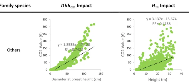
29
Family species
𝑫𝒃𝒉𝒄𝒎Impact
𝑯𝒎Impact
Others
Table 7: Diameter at breast height and Height impact, by species family
Positive relation is observed for the both variables. When 𝑑𝑏ℎ𝑐𝑚 and ℎ𝑚 increase the credit of 𝐶𝑂2
value increases. These behaviours not necessarily look a linear relationship between both variables and 𝐶𝑂2. Once the R-squared value is higher than 70% this contribute to our linear relations between
the variables, because generally considered strong effect size. We can observe this aspect relatively to 𝐷𝑏ℎ𝑐𝑚 to family Aceraceae, Malvaceae, Betulaceae, Fagaceae, Platanaceae family species. The Malvaceae present the higher R-square value for both variables. Attending to this family, a 10cm
increase in 𝑑𝑏ℎ𝑐𝑚 will increase 𝐶𝑂2 by 0.050 €, Equally, a 10cm increase (10%) in ℎ𝑚 will increase the
amount of 𝐶𝑂2 by (0,082)€The negative value, relative to 𝐶𝑂2, may indicate the high oxygen
consumption by this species. To better preview the variables impact on the CO2 we had computed the equation derivatives [Appendix 7].
∆ 𝐶𝑂2= 0.0141(10𝑑𝑏ℎ𝑐𝑚) − 0.0907 = 0.0141(10) − 0.0907 ≈ 0.050 €;
∆ 𝐶𝑂2= 0.0492(ℎ𝑚+ 10%) − 0.1683 = 0.0492(1.6 × 1.10) − 0.1683 ≈ −0,082€;
We can observe a higher difference between the variables impact. The presented values correspond to the expected values. Since trees have a higher number and volume of leaves in their branches, it is expected that the 𝑑𝑏ℎ𝑐𝑚 has a greater impact compared to ℎ𝑚. Therefore, the higher 𝑑𝑏ℎ𝑐𝑚 values
will increase the volume trees and the 𝐶𝑂2 credit.
To clarify reasons for different 𝐶𝑂2 amounts it is useful to examine differences among species that are
most important by virtue of their abundance and size. For example, Tilia Tomentosa is not the most plentiful species, but it assumes the most 𝐶𝑂2 credit in accordance with all our equations.
There are no discernible trends in terms of a set of equations always producing 𝐶𝐾𝑔 estimation that is
the highest or lowest across all species. The
𝑑𝑏ℎ𝑐𝑚 and height impact will depend the equation used, but we can observe a positive impact in all
of them. Attending to the species with more contribution to the 𝐶𝑂2, like Tilia Tomentosa, Fagaceae Quercus Spp and populus nigra ‘italica’, we can observe a relation closer to linear. So, the higher trees
dimension values, the higher 𝐶𝑂2 credit.
y = 1.3535x - 17.128 R² = 0.7422 0 50 100 150 200 250 300 350 0 50 100 150 CO2 Valu e (€)
Diameter at breast height (cm)
y = 3.137x - 15.674 R² = 0.4158 0 50 100 150 200 250 300 350 0 10 20 30 40 CO2 Valu e (€) Height (m)