* This thesis was written in accordance to the Master thesis guidelines of Maastricht University and is part of the
Urban Population Growth in Europe: The Attractiveness of Smart Cities
Master Thesis*
by Philipp Haese i6033213 / 773
Universidade Nova de Lisboa
Nova School of Business and Economics Supervisor: Sofia Margarida Fernandes Franco
Maastricht University
School of Business and Economics Supervisor: Pierpaolo Parrotta
Lisbon
Table of Contents
1. Introduction ... 1
2. Literature Review ... 2
2.1. US Based Studies on Migration ... 2
2.2. European Based Studies on Migration ... 4
2.3. Smart Cities Studies ... 7
3. Analytical Model ... 8
3.1. Households’ Behavior ... 9
3.2. Firms’ Behavior... 11
3.3. Urban Population Growth Rates ... 12
4. Data and Estimation ... 13
4.1. Sample Characteristics ... 13
4.2. Variables ... 14
4.3. Empirical Methodology ... 17
5. Results and Robustness Tests ... 18
5.1. Reference Model Results ... 18
5.2. Pooled OLS Results and Discussion ... 19
5.3. Tests of Model Specification and Robustness ... 23
6. Conclusion ... 26
Appendix A. Supplemental Figures ... 28
Appendix B. Supplemental Tables ... 30
1. Introduction
Cities around the world continuously compete for mobile workers and investment as these represent the basis of their regional economic development. Thus, the attraction and retention of businesses and households are central goals of urban policies (Malecki, 2004). To stay competitive, local governments and municipal planners attempt to understand which factors determine the attractiveness of metropolitan areas towards migrants. As European countries face severe demographic changes, such as overall population decline and ageing, this subject gains additional importance.1
In their location decision, mobile households compare economic and non-economic conditions across potential destinations to assess which place will maximize their welfare. Within the European context, several studies have shown the importance of local labor markets and regional wealth as migration incentives (Cheshire and Magrini, 2006; Biagi et al., 2011). In addition, quality of life (QOL) considerations
represent a set of potential push- and pull-factors for migration. They arise from the presence of amenities, which are local attributes such as cities’ social and physical environment, governmental policies as well as public goods and services.
This thesis investigates the effect of amenities associated with the emerging field of Smart Cities on the attractiveness of European metropolitan areas towards migrants. The term Smart City describes urban development concepts that invest in human and social capital as well as in conventional and modern infrastructure to generate sustainable economic growth and a high quality of life (Caragliu et al., 2009). Giffinger et al. (2007) identify six domains that provide opportunities for the application of Smart City concepts: economy, people, governance, mobility, environment, and living. We refer to the outcome of investments into these areas as smart amenities which canbe of inter alia, cultural, sociodemographic and infrastructural nature. Earlier studies operationalized the concept of Smart Cities into sets of measurable indicators and used them to create comparative rankings of cities (Giffinger et al., 2007; Neirotti et al., 2014). While these studies help us measure cities’ level of ‘smartness’, their results are based on subjective opinions and do not provide a quantitative measurement of the magnitude of the effects of these variables on migration levels and urban attractiveness. Thus, this thesis aims to contribute to the research on Smart Cities by applying insights from studies that examine inter-urban competition based on migration flows. In particular, we assess the relationship between the availability of smart amenities and the population balance of European metropolitan areas. We employ cities’ population balance as a measure of urban attractiveness, which provides an objective assessment of cities’ quality of life and has a strong theoretical foundation.
We hypothesize that, ceteris paribus, the local availability of smart amenities is positively correlated with urban population growth rates, which would be indicative of the utility that they generate from migrants’ perspective. For this purpose, we construct and analyze a panel dataset of 76 European metropolitan areas, which have 500.000 inhabitants or more, for the period between 2002 and 2013. We control for economic, sociodemographic and natural amenity-based determinants and we estimate the effect of smart amenities on cities’ population change. Our results suggest a positive correlation between population growth rates and the local presence of highly skilled individuals, recreational areas and infrastructure for non-motorized transport. Our pooled OLS specification is compared to alternatives with lower multicollinearity or reduced unobserved heterogeneity and provides the best goodness of fit. We conclude that the application of Smart City development concepts enhances the attractiveness of European metropolitan areas towards migrants. Further, our results suggest that migration flows within the EU react to perceived differentials in metropolitan areas utility levels and support the existence of European amenity-based migration.
The thesis is structured as follows. Section 2 provides a literature review of US-based and European-based studies on migration that provide the theoretical foundation for our research. Additionally, we review Smart City studies to outline the aforementioned literature gap. Section 3 introduces the spatial equilibrium framework, which underlies our empirical methodology as well as the necessary assumptions to use population growth rates as an indicator of households’ revealed preferences. We provide a detailed description of our data sources, selected variables and empirical framework in Section 4. Section 5 presents and discusses our results and robustness tests. Finally, Section 6 concludes.
2. Literature Review
2.1. US Based Studies on Migration
Empirical research examining inter-urban competition through the location decisions of households and firms originates from Tiebout (1956). According to the Tiebout setup, mobile workers within a single labor market compare perceived utility differentials across locations and relocate to improve their welfare. By ‘voting with their feet’, individuals reveal their preferences about a region’s or city’s attractiveness. This led to the investigation of how location-specific characteristics determine the ability of a place to attract people, what weight decision makers assign to them and whether they change over time.
non-traded goods. Under the models’ assumptions, all economic agents relocate if they expect that it will improve their welfare.2 For areas with population inflow, this continuous migration process increases
housing prices while decreasing wages, which will generate a state of spatial equilibrium where individuals with identical preferences enjoy the same utility level across all locations. Consequently, households in places with lower amenities are compensated through higher nominal wages or lower costs of living while firms in less productive places are compensated through lower labor or non-labor costs. Following this framework, several studies for the United States have shown that regional differences in economic conditions and amenities influence migration decisions and therefore population growth (Gyourko and Tracy, 1991; Albouy, 2008; Chen and Rosenthal, 2008).
For instance, Gyourko and Tracy (1991) investigate the effect of spatial characteristics on households’ location decisions by estimating the contribution of fiscal policies, public services as well as climate and natural environment on quality-adjusted houseing prices and quality-adjusted wages.3 For a sample of 130
cities, they show that these characteristics explain a large share of the observed variation in prices and wages, 55% and 44% respectively. On average, households are willing to forgo $8,227 of yearly income to live in the city with the highest observed level of amenities compared to the city with the lowest level. This significant discrepancy between cities suggests that households consider economic and non-economic factors in their location decision. In particular, the authors emphasize the role of spatial differences in economic conditions because cities can influence their attractiveness by creating favorable fiscal policies and public services.
Similarly, Albouy (2008) recognizes the importance of adjusting incomes for federal tax rate. He further extends the Rosen-Roback model to include non-housing prices in household consumption and to account for household’s non-labor income. His analysis of US Census data from 276 Metropolitan Statistical Area shows that households are willing to forgo significant amounts of income to live in areas with better natural amenities.4
This estimation and similar ones are sensitive to the choice of amenities included in the model. Therefore, Chen and Rosenthal (2008) construct an index, which compares wages with rents and only
2 The Rosen-Roback model requires a set of strong assumptions, such as labor and capital can move immediately and free of charge, wages equal the marginal productivity of labor (firm equilibrium) and housing prices are equal to the costs of providing housing (housing market equilibrium). For details, see Rosen (1979) and Roback (1982).
3 The authors apply a large set of explanatory variables for fiscal policies (e.g. income tax, state corporate tax rates, effective local property tax rate), public services (per capita incidents of violent crime, insurance company local premium, number of hospital beds per 1,000 people, student/teacher ratio) as well as climate and environment (e.g. average annual precipitation; relative humidity; average wind speed; sunshine days, heating and cooling degree days, mean total suspended particulates, closeness to an amenity).
controls for worker and housing characteristics, in order to implicitly measure the value of all observed and unobserved amenities. The authors construct a panel of separate measures for the location preferences of households and firms and show that these are only modestly correlated, which implies that both groups value different location-specific attributes. Specifically, their ranking suggests that the average household prefers to live in warm coastal regions, while the average firm prefers to locate in large, growing cities. Interestingly, an analysis of household characteristics reveals that workers and in particular high-skilled workers seek cities that are also attractive to businesses. Although these studies have provided evidence that households and firms in the US are willing to trade off favorable economic conditions for higher levels of amenities, we cannot easily generalize these country-specific findings to a European context.
2.2. European Based Studies on Migration
In contrast to the US, population movements in Europe involve migration flows between countries, which are subject to large linguistic, cultural and institutional differences. This interregional heterogeneity creates additional barriers for people to relocate and results in a more ridged labor market, which is potentially slower to react to spatial differences in economic factors such as wages and employment opportunities. For instance, between 1976 and 2013, the adjustment to a one-standard error positive labor demand shock on average required ten years in Europe compared to five years in the US (Beyer and Smets, 2015). In addition, interregional net migration flows show that during each year of the 1990s 0.04% of the European population has relocated, which is more than one order of magnitude less than the US’s mobility rate of 0.5% (Cheshire and Magrini, 2006). As a result, the assumption of perfect factor mobility – common in US-based models – is challenged and it is feasible that large economic discrepancies persist across regions and countries of the EU. Within-country and cross-country level studies of migration choice provide mixed evidence on whether this assumption is satisfied in the European context.
For instance, in a study of 71 German cities, Buch et al. (2013) regress each locations’ net migration rate on labor market conditions and a set of amenities. They address unobserved time-invariant city characteristics and potential reverse causality between migration and the explanatory variables through city fixed effects, the use of predetermined explanatory variables and instrumentalization of labor market conditions.5 Based on data from 2000 to 2007, the authors estimate a significant effect of recreation areas
such as urban green spaces, climatic conditions and access to transportation networks on cities’ labor migration balances. However, they do not find support for a favorable effect of human capital on the urban
5 The authors apply the share of older workers, a weighted average of nation-wide employment growth by branches
migration. The authors conclude that amenities act as a national migration driver once economic factors have been controlled for, which suggests that economic discrepancies that exist between Germany’s east and west partially compensate for differences in local non-economic features.
These findings contrast with Biagi et al. (2011), who utilize a dataset of Italy for 2001 and 2002, which allows them to determine the geographic distance associated with each migration movement. They use this information to separate inter-regional migration flows into their long- and short-distance components and estimate the effect of economic variables and amenities on them separately.6 The authors provide evidence that regional differences in GDP and employment rate determine long-distance migration patterns whereas natural amenities such as the vicinity of a coastline are only important for short-distance migration decisions. We observe that local amenities do not have an effect on migration decisions within the country as a whole but only within distinct regions, which suggests that it is possible that regional economic differences persist even within highly integrated economic area.
A comparison of the previous studies leads us to assume that migration mechanisms might structurally differ between countries. Culture and other country-specific factors potentially affect people to assign different weights to economic and non-economic factors. This represents an a caveat of cross-country migration studies in the EU as they have not been able to account for the geographic origin of population flows yet (Cheshire and Magrini, 2006; Rodríguez-Pose and Ketterer, 2012). Due to data limitations, these studies have focused on investigating the location decisions of the aggregated flow of migrants.
For example, Cheshire and Magrini (2006) regress net migration rates of 121 major EU Functional Urban Regions (FURs) between 1980 and 2000 on a set of economic and non-economic determinants.7 They include controls for industrial structures measured by historical employment levels in industry and agriculture as well as coal mining and port activity as these negatively influence a location’s natural and social environment. Further, the authors assume that the process of European integration generates cross-country heterogeneity as it systematically favors core regions.8 Their results show that spatial income differences, which are interpreted as a consequence of the change in economic potential, are positively correlated with net migration.9 Specifically, during the observed period, a one-unit increase in the squared
6 Here, long-distance migration is defined as the population flow from provinces belonging to the country’s “north” to its “south” and vice-versa. All other population flows are considered as short-distance.
7 Functional Urban Regions are defined based on the construction of a commuting zone around a core city, subject to population and density thresholds. They attempt to capture the concept of Metropolitan Statistical Areas (MSA) commonly used in the United States. For more detail, see Cheshire and Hay (1989). The analysis excludes FURs with a population of less than 333.000 or with a core city of less than 200.000 during all years between 1951 and 1981. 8 In this context, the term “core regions” refers to the continent’s most industrialized cities. Their economies are best positioned to benefit from decreasing transportation costs, EU enlargements and market liberalizations.
measure of integration gain is associated with an approximately 0.2% increase a city’s population growth rate.
Non-economic differences between FURs are captured by a location’s geographic position
based on latitude and longitude as well as its climate, which is operationalized by frost frequency,
temperature and number of wet days. When implemented as values relative to the EU as a whole,
these variables display no significant effect. However, relative to the same country, these measures
are correlated with net migration rates and serve as a predictor of within-country population
movements. Migrants appear to choose a country based on economic factors first and then opt to
live in a region with good climate, which suggests that cross-country migration is primarily a
reaction to economic discrepancies.
Rodríguez-Pose and Ketterer (2012) are the first to present evidence that natural and man-made amenities strongly influence location choices between all regions of the EU. Their analysis is based on 133 administrative divisions of EU15 countries (NUTS1 and NUTS2 regions) and covers the years between 1990 and 2006.10 The use of NUTS regions enables a comprehensive estimation of the impact of natural
amenities.11 In contrast to Cheshire and Magrini (2006), the authors conclude that places with pleasant
climate, nature conservation areas and cultural services are comparatively more successful at attracting migrates – even across European boarders. These empirical findings are in line with Partridge's (2010) prediction that rising standards of living, ongoing economic integration as well as declining migration and information costs will increase the weight that Europeans assign to amenities in their location choices. Rodríguez-Pose and Ketterer's (2012) analysis further includes a “social filter”, which aggregates several sociodemographic elements, such as the level of human capital endowments and inverse share of employment in agriculture. In contrast to Buch et al. (2013), the authors find a significant effect of these measures on urban attractiveness.
While early European-based studies of migration provide evidence for the existence of large economic discrepancies between counties and regions, which have been the primary migration driver at that time, studies that are more recent highlight the importance of natural and man-made amenities in determining regional attractiveness. This suggests that migrants in the EU might value the same location-specific attributes as their US counterparts.
10 Defined by the European Commission, the NUTS classification (Nomenclature of Territorial Units for Statistics) hierarchically divides the economic territory of the EU. NUTS 1 are “major socio-economic regions” and NUTS2 are “basic regions for the application of regional policies” (http://ec.europa.eu/eurostat/web/nuts/overview; last visit September, 2015).
2.3. Smart Cities Studies
A further strand of literature that relates to the previous two sets of studies is the research on Smart Cities, which aims to identify technical, economic and social innovations that improve the efficiency and QOL in urban spaces. Over the last 15 years, a variety of stakeholders with different interests contributed to this emerging discussion (i.e. technology vendors and integrators, city officials and policymakers as well as think tanks and academic researchers), which led to a wide dispersion of topics within the field. Among these, we are primarily interested in studies that help us to understand how a city’s level of smartness can be determined empirically and how it relates to their urban performance and QOL.
For instance, Giffinger et al. (2007) operationalize the concept of smartness by identifying a set of measureable performance indicators, which they use to create a comparative ranking of 70 medium-size European cities.12 This ranking is an attempt to identify role models for the development and
implementation of smart initiatives and presents insights into how cites attempt to increase their competitiveness. Giffinger et al.’s framework considers six domains to characterize the smartness of a city: economy, people, governance, mobility, environment and living. These are broken-down into 31 factors, which are measured through 74 indicators available on the regional-level and national-level. In order to express a city’s level of smartness numerically, the authors aggregate the standardized values by assigning equal weights to all variables. This highlights the fact that we are not yet able to estimate the relative importance of different smart characteristics on urban performance. Further, the applied indicators capture both, investments into smart initiatives as well as their outcomes. Therefore, the subsequent ranking can be interpreted partially as a city’s effort and success at implementing smart initiatives.13 The authors declare
Luxemburg to be number one and further show that hardly any city scores above average in all six domains, which suggests that cities develop distinct profiles according to their needs.
Neirotti et al. (2014) introduce contextual conditions as determinants for the development of these distinct profiles in a study of 70 international, self-proclaimed ‘smart cities’, 25 of which are located in Europe. Their methodology estimates the impact of four groups of contextual conditions, which are measured by variables related to a city’s size and demographic density, economic development, technology development as well as environmental policies, on a city’s progress in six domains that characterize smartness. The set of domains is nearly identical to Giffinger et al.'s (2007), however, the authors rely on
12 The authors’ sample includes all European cites with a population between 100,000 and 500,000 that have at least one university and a catchment area of less than 1.500,000.
an coverage index to judge a city’s success.14 Their analysis reveals that the number of domains addressed
by a city is independent of its size, however, which domains are addressed is depended the city’s geographic region. American and Asian cities tend to make higher investments in infrastructure such as transportation, electricity and telecommunication networks, whereas European cities focus on human capital and government practices. Regardless of the region, there is a significant and positive effect of population density on infrastructure investments. The authors conclude that there is no dominate model as city development is need-based and path depended.
These studies represent valuable contributions because they provide a first attempt at operationalizing the concept of Smart Cities into measurable indicators. However, they are inherently prone to a high level of subjectivity in the choice of variables and their approach is restricted to comparatively ranking a selected number of cities. This prevents us from interpreting their findings outside their specific settings.
This thesis aims to address some of the challenges that arise in the surveyed literature by further investigating the relationship between the presence of smart amenities and the urban attractiveness of European cities. Thus, we express urban attractiveness as a city’s population growth rate and analyze its correlation with measures of smart amenities. In contrast to earlier Smart City studies, which compare selected performance indicators to asses a city’s level of smartness, this represents an attempt to understand the impact of these indicators on a more general objective of urban planners.
For this purpose, we introduce a conceptual framework based on the locational choice spatial equilibrium approach of European based migration studies. Specifically, we follow Rodríguez-Pose and Ketterer (2012) and model net migration as the reaction of households and firms to differences in economic and non-economic regional characteristics. To the best of our knowledge, this methodology has not been applied in studies of Smart Cities, yet. However, it might be able to advance our understanding of cities’ returns to investments into smart initiatives by relating them to a measure of urban competiveness, which is firmly based on economic theory.
3. Analytical Model
To derive our hypothesis about the relationship between urban population growth rates and the presence of smart amenities, we develop a spatial equilibrium framework based upon Brueckner (2011). In the long run the welfare of economic agents is equalized across all locations so that in equilibrium economic agents (firms and households) are indifferent where to locate. During the transition towards this equilibrium state, households and firms relocate to metropolitan areas that provide higher-than-average utility or profits. We
consider the resulting migration flows as an indicator of local differences in economic and non-economic conditions.
3.1. Open City Model Setup
We assume an open city model where population is homogenous, rational and perfectly mobile where all agents choose to locate in their preferred metropolitan area, which are indexed by i, i = 1, …, N. Each metropolitan area i has an exogenously given level of amenity endowments (𝑍𝑖). For simplicity, we assume that the total amount of households (P), theamount of firms per metropolitan area (𝐹𝑖)and the amount of available square meters of real estate per metropolitan area 𝐿𝑖 are fixed.The demand for real estate by households and firms is endogenously determined as a result of their individual optimization problems. Metropolitan areas’ population stock (𝑃𝑖) is endogenously determined by migration across cities. Further, we assume that both the real estate and the labor markets are competitive. Consequently, the price per unit of housing consumption (𝑝𝑖) reflects the cost of real estate and the local wage level (𝑤𝑖) reflects workers productivity. For simplicity, we do not take into account agglomeration economies or congestion frictions and only allow for within-city commuting but not for between-city commuting.
3.1. Households’ Behavior
Households’ location-specific utility is derived from the consumption of a traded good (𝑇𝑖), for which the price is normalized to one, the consumption of real estate for housing (𝐿𝐻𝑖) as well as the presence of non-pecuniary amenity-based features (𝑍𝑖). We assume that each household provides one unit of labor at nominal wage (𝑤𝑖). Thus, their utility maximization problem is given by:
max 𝑈𝑖 = 𝑈𝑖(𝑇𝑖, 𝐿𝐻𝑖, 𝑍𝑖,) (1)
𝑠. 𝑡. 𝑤𝑖− (𝑇𝑖+ 𝑝𝑖𝐿𝐻𝑖) ≥ 0 (2)
𝐿𝐻𝑖 ≥ 0, 𝑇𝑖 ≥ 0,
where consumption of traded good 𝑇𝑖 is the numeraire and 𝑝𝑖 is the price per unit of housing consumption. Households choose the utility maximizing level of 𝐿𝐻𝑖 and 𝑇𝑖, with respect to their budget constraint (1). Solving this problem provides the demand curve of households for real estate, which we denote as:
𝐿𝐻𝑖(𝑝
Substituting (3) and the demand curve for consumption of traded good 𝑇𝑖 into (1), we show that households’ indirect level of utility from living in metropolitan area i depends on the local wage level (𝑤𝑖), the price per unit of housing (𝑝𝑖) and levels of amenities (𝑍𝑖):
𝑉𝑖(𝑝𝑖, 𝑤𝑖, 𝑍𝑖)
−, +, + . (4)
Indirect utility increases in the local wage level (𝑤𝑖), as it enables households to consume more, and decreases in the local price per unit of housing (𝑝𝑖), which constraints households’ budgets. As indicated by the comparative statics, the level of amenities is measured positively, for example through variables that capture cities’ level of safety instead of their crime rate, and thus indirect utility increases in 𝑍𝑖.15 We consider households’ utility as synonymous to “happiness” and QOL. Since households are perfectly mobile they need to derive the same utility level 𝑉̅ from living in city i as in any other city. In other words, they need to be indifferent about their location. Otherwise, they will relocate to a place, which is more attractive in terms of economic and non-economic features. Consequently, the equilibrium condition, which governs households’ behavior, is that utility must be equal across all metropolitan areas:
𝑉𝑖 = 𝑉̅ = (𝑉1, … , 𝑉𝑁)/𝑁, (5)
where 𝑉̅ is the average indirect utility level across all metropolitan areas, which is exogenously determined as the Nth share of “total available QOL”. In the state of the spatial equilibrium, housing prices and wages vary across metropolitan areas to compensate for differences in local amenity levels (Roback, 1982). Further, for a given level of amenities, high housing prices compensate for high wages level to equalize the metropolitan area’s indirect utility level to the average 𝑉̅ and vice versa.
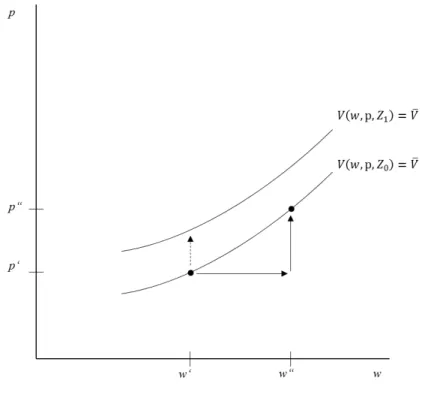
We illustrate this compensating-differential argument in Appendix Figure A1, which shows two indifference curves for different amenity levels. Both curves represent the utility level 𝑉̅ and are upward sloping because an exogenous shock to the wages from w’ to w’’ will be compensated by an increase in housing prices from p’ to p’’. Further, indirect utility derived from amenities is higher in the upper curve as
𝑍1> 𝑍0. Therefore, either wages or housing prices need to adjust to cancel out the additional utility. For example, the dashed vertical arrow represents an exogenous shock to a city’s level of amenity endowments. As the area temporarily provides above-average levels of indirect utility, households relocate towards it and increase its population stock. Consequently, the demand for housing and the supply of labor increase, which increases housing prices and decreases wage levels to equalize the indirect utility level to the metropolitan average 𝑉̅.16 To determine the actual variation of housing prices and incomes to different levels of amenities
15 For further information on comparative statics, see Brueckner (2011).
we introduce assumptions about firms’ behavior.
3.2. Firms’ Behavior
Firms’ adjustment process to spatial differences in economic and non-economic features occurs similarly to households’ behavior. Without specific assumptions about the form of firms’ production function, we assume that they use commercial real estate (𝐿𝐹𝑖) and labor (𝑊𝑖) as inputs to produce an exogenously given output level (𝑄𝑖) of the traded good. Location-specific wages (𝑤𝑖) and the price per unit of commercial real estate (𝑝𝑖) reflect the factor prices.17 Firms’ cost minimization problem is given by:
min 𝑝𝑖𝐿𝐹𝑖 + 𝑤𝑖𝑊𝑖, (6)
𝑠. 𝑡. 𝑓(𝐿𝐹𝑖, 𝑊𝑖) = 𝑄𝑖 (7)
𝐿𝐹𝑖 ≥ 0, 𝑊
𝑖 ≥ 0
Further, from firms’ point-of-view, amenities (𝑍𝑖) describe local exogenous features such as the natural or socioeconomic environment, the regulatory system and public services. These features influence productivity and we assume that firms benefit from their presence.18 Under consideration of amenities,
minimizing (6) subject to (7) results into firms’ demand curve for real estate:
𝐿𝐹𝑖(𝑝𝑖, 𝑤𝑖, 𝑍𝑖). (8)
Substituting (8) and the demand curve for labor into (6), we show that firms’ cost function for production in metropolitan area i depends on the local wage level (𝑤𝑖), the price per unit of housing (𝑝𝑖) and levels of amenities (𝑍𝑖) as follows:
𝐶𝑖(𝑤𝑖, 𝑝𝑖, 𝑍𝑖, )
+, +, − . (9)
Consequently, firm’s profits from production in metropolitan area i are given by:
Π𝑖(𝑤𝑖, 𝑝𝑖, 𝑍𝑖, ) = 𝑄𝑖[𝑘𝑖− 𝐶(𝑤𝑖, 𝑝𝑖, 𝑍𝑖)],
−, −, + (10)
where 𝑘𝑖 = 1 is the price of the traded good and 𝑄𝑖 is omitted for simplicity. Analogous to households, firms are perfectly mobile and spatial equilibrium requires that profits are equalized across metropolitan areas:
Π𝑖 = Π̅ = (Π1, … , Π𝑁)/𝑁, (11)
where Π̅ is the average profit level among all metropolitan areas, which we set equal to zero for
17 For simplicity, our analytical model does not differentiate between residential and commercial land use. Therefore, we use 𝑝𝑖 to refer to general land prices, cost of commercial land use and cost of private housing.
simplicity. This implies that in equilibrium, firms are indifferent in their location choice. Given a region’s level of amenities, low real estate prices compensate firms for high wage levels and vice versa. Further, land prices and wages vary across metropolitan areas to compensate for differences in local amenity levels. The iso-profit curves in Appendix Figure A2 illustrate how a higher level of amenities, which reduces production costs, requires higher real estate prices or wages to equalize local profits to zero. If a metropolitan area temporarily offers superior per unit costs, for example, through comparatively low wages or land prices or by comparatively high productivity, it experiences an influx of businesses. This process bids up the city’s wage level and land prices until firms’ expected lifetime profits equal zero again. Appendix Figure A3 illustrates households’ indifference curves and firms’ iso-profit curves. Their intersection indicates a metropolitan areas’ equilibrium real estate price and wage level. Under the assumption that firms’ unit costs only slightly decrease in amenities 𝑍𝑖, we expect a high-amenity city to have high real estate prices and high wage levels.
3.3. Urban Population Growth Rates
We assume that the physical extent of each metropolitan area is fixed and that the available real estate is distributed between households and firms according to their demand curves (3) and (8):
𝐿𝑖 = 𝐿𝐻𝑖(𝑝𝑖, 𝑤𝑖, 𝑍𝑖) ∗ 𝑃𝑖+ 𝐿𝐹𝑖(𝑝𝑖, 𝑤𝑖, 𝑍𝑖) ∗ 𝐹𝑖 (12) Solving for metropolitan areas’ level of population (𝑃𝑖) reveals that it is a function of the local wage level
(𝑤𝑖), the price per unit of housing (𝑝𝑖) and the amenity level (𝑍𝑖):
𝑃𝑖(𝑝𝑖, 𝑤𝑖, 𝑍𝑖) =𝐿𝑖− 𝐿𝑖 𝐹(𝑝
𝑖, 𝑤𝑖, 𝑍𝑖) ∗ 𝐹𝑖
𝐿𝐻𝑖(𝑝𝑖, 𝑤𝑖, 𝑍𝑖) (13)
We further divide (13) by 𝑃𝑖,𝑡−1 and take logarithms on both sides to approximate urban population growth rates:
𝑃̂ (𝑝𝑖,𝑡 𝑖, 𝑤𝑖, 𝑍𝑖) = 𝑙𝑛(𝑃𝑖,𝑡) − 𝑙𝑛(𝑃𝑖,𝑡−1) = 𝑙𝑛(𝐿𝑖,𝑡− 𝐿𝐹𝑖,𝑡) + 𝑙𝑛(𝐹𝑖,𝑡) − 𝑙𝑛(𝐿𝑖,𝑡𝐻) − 𝑙𝑛(𝑃𝑖,𝑡−1) (14) Based on the equilibrium conditions outlined in Section 3.1. and 3.2., we assume that a positive shock to amenity levels increases a metropolitan areas’ population stock, real estate prices and wage levels. Ceteris paribus, higher levels of amenities 𝑍𝑖 are positively correlated with population growth. This is consistent with Tiebout’s (1956) notion that migration flows are the aggregation of households’ revealed preferences regarding the level and quality of location-specific characteristics. Households ‘vote with their feet’ and reveal their preferences about metropolitan areas by moving from low-utility cities to high-utility cities. We hypothesize that, ceteris paribus, the local availability of smart amenities is positively correlated with migration rates, which would be indicative of the utility that they generate.19
19 Migration flow are the net change in population stock of city i between t-1 and t: 𝑀
4. Data and Estimation 4.1. Sample Characteristics
Our empirical analysis builds on a panel dataset of 76 metropolitan areas, which have 500.000 inhabitants or more and are located within the EU-15 countries and Switzerland.20 Time intervals are measured in
years and cover the period between 2002 and 2013. The data has been collected from three different sources: the OECD Metropolitan Database, the ESPON 2013 Database and the fifth and most recent round of the Eurostat Urban Audit. These projects gather metropolitan level data on various social and economic dimensions in OCED and European countries. As these sources differ in their definition of metropolitan areas, we performed the following modifications to compile them into a comparable dataset.
Functional Urban Areas (FUA), which correspond to the OECD’s definition of ‘a metropolitan area’, are our main spatial unit of analysis. They include cities with an urban core that satisfies a minimal density threshold (1.500 inhabitants per km²) and a minimal population threshold (50.000 inhabitants) as well as the surrounding commuting zone, which are constructed based on commuting patterns.21 Most cities are
part of their own commuting zone or a polycentric commuting zone covering multiple cities. In particular, for larger cities these hinterlands represent labor markets that are highly integrated with the cores. The definition of cities and greater cities (CGC) does not include these worker catchment areas but is otherwise identical with FUA (Dijkstra and Poelman, 2012).22 To establish a comparison between data that was
collected under these two definitions, we transformed all non-climate CGC variables into rations, e.g. share of high-skilled individuals of the total metropolitan population, and use them as proxies for the corresponding FUA values. Another set of variables included in our analysis is only available based on national administrative subdivisions (i.e. NUTS3).23 To approximate the FUA level, we aggregated these
indicators based on their correspondence with metropolitan regions.24 Further, we imputed a number of data
𝑑𝑖,𝑡, where 𝑏𝑖 is the fertility rate and 𝑑𝑖 is the mortality rate. However, as we explain further in Section 4.2., we assume that 𝑏𝑖,𝑡= 𝑑𝑖,𝑡 and surrogate migration flows through population growth rates.
20 The term EU-15 refers to the 15 Member States of the European Union as of December 31, 2003: Austria, Belgium, Denmark, Finland, France, Germany, Greece, Ireland, Italy, Luxemburg, Netherlands, Portugal, Spain, Sweden, and the United Kingdom. Due to data constraints, Greece and Luxemburg have been excluded from o sample.
21 Specifically, an urban center is defined based on adjacent 1-km² grid cells, which fulfill the minimum density and population threshold. Then, FUA boundaries are delimitated around this center based on Local Administrative Units - Level 2 (LAU2), such as municipalities, with at least half their population inside the urban center. The commuting zone is constructed from all contiguous LAU2 that have 15% or more of their employed resident population working in the urban core. For more details, see OECD (2012).
22 CGC are build based on the same definition of a core city as FUA. FUA extend the definition of CGC by the
inclusion of a commuting zone and have formerly been referred to as Large Urban Zones (LUZ). For more details, Dijkstra and Poelman (2012).
23 As defined by the European Commission, the nomenclature of territorial units for statistics (NUTS) classification is a hierarchical system for dividing the economic territory of the EU and Level 3 correspondents to small regions.
points to increase our efficient sample size.25 While these missing values potentially indicate a nonrandom
sample, we believe that they are produced by exogenous sample selection, i.e. more efficient municipalities are able to provide complete data. In this case, the attrition would be based on an unobserved independent variable and the sample selection itself will not introduce bias or inconsistency to our estimations.
4.2. Variables
The dependent variable of all estimations is cities’ population growth rate. In the absence of adequate data for fertility and mortality rates at a metropolitan level, we assume that each year both rates are equal for a given city and subsequently proxy for net migration rates through annual growth rates of population size.26
In addition to decreased data demands, population growth offers an advantage above net migration rates in capturing urban utility differences in cities, which have high rates of net migration and low rates of natural labor force growth or vice versa (Faggian et al., 2012).27 As outlined in Section 3, we assume cities’
endowments of location-specific characteristics to determine migration flows. These characteristics represent our independent variables and are grouped into three categories: economic, sociodemographic and amenity-based. We separate amenity-based regressors further into natural amenities and smart amenities.
Economic migration determinants are captured using inter-urban differences in standards of living and labor market conditions. Specifically, we control for cities’ annual GDP per capita and its growth rate as well as for locational-specific differences in unemployment rates. In addition, we indicate whether a city is a country’s capital as they traditionally provide a comparatively attractive labor market. Based on our conceptual framework, we expect that urban areas with relatively poor economic conditions have on average a lower population inflow and vice versa.
Analogous to Rodríguez-Pose and Ketterer (2012), we attempt to account for sociodemographic
capital city status, border and coast presence as well as the number of IP address per capita from NUTS3 to FUA. We applied equal weights to components. In the case of binary variables, resulting values larger than one were condensed to exactly one. (http://ec.europa.eu/eurostat/documents/4313761/4311719/Correspondence_NUTS2010_ID-Metroregions+_03-12-2014.xls/ca9628ba-588d-4426-97d5-d4dbba61218b, last visit November, 2015)
25 For all indicated variables (Table 1), we have applied forwards imputation. Missing observations during one sample period were replaced by their last observed value, which reflects our assumption that if a measurement is missing it has not changed from the last time it was observed. Further, we applied a moving average filter to smooth imputed values. Specifically, we used an MA(3) filter for the current and two backwards periods under uniform weights. 26 The data shows that the size of both rates is reasonably close. The Pearson's correlation coefficient between population growth and net migration rate is 0.9579 for the observations within our sample that provide the necessary data, N = 464.
externalities that we expect to influence cities’ economic potential. Specifically, we control for age structures, which we proxy through the share of the total population aged 15-24. We consider this measure influential because it reflects the flow of human resources into the labor market and, consequently, the renewal of the existing stock of knowledge and skills (Rodríguez-Pose and Crescenzi, 2008). The inclusion of further sociodemographic controls and, in particular, the share of total employment in the agricultural sector would be desirable, as they could provide a measure for cities’ productive employment of human resources and their level of hidden unemployment.
Natural amenities, such as climate, geography and air quality, have been proposed as another set of migration drivers. We introduce controls for cities’ annul average of daily sunshine hours and average winter temperatures, while we exclude their annual amount of precipitation and average summer temperature due to high levels of correlation with the aforementioned variables. Despite ongoing global climatic change, both measures are expressed as averages over the period 1990-2013 and included as time-constant regressors. In addition, we control for the presence of borders and coastlines through a binary indicator. Finally, we proxy for air quality through the annual average accumulated concentration of ozone and the average nitrogen dioxide (NO2) concentration. At ground level, both of these particles are considered harmful air pollutants and are a direct or indirect product of industrial activities and traffic (Fenger, 1999). Consequently, they might not be exogenous from factors such as population density and migration.
Smart amenities lie at the core of our analysis and are associated with the application of Smart City development concepts to the domains: people, living, mobility, economy, environment and governance (Giffinger et al., 2007).28 We introduce a set of proxy variables to investigate their relationship with
migration rates.
Smart People: Level of human capital is captured by the population’s share of high-skilled, i.e. the share of the total population aged 25-64 with ISCED level 5 or 6 as the highest level of education.29 While
this variable primarily reflects households’ private decisions, we believe that cities are able to influence this
28 According to Giffinger et al. (2007), Smart People comprises a city’s human and social capital as can be observed in the population’s level of education and the quality of social interactions regarding integration and public life. Smart Living addresses a city’s quality of life in a narrow sense, such as the presence and quality of recreation areas, culture, health, safety, housing and tourism. Smart Mobility is described by a city’s local and international accessibility and its transport systems. Smart Environment is characterized by natural resource management and environmental protection policies. Smart Economy includes factors associated with economic competitiveness such as innovative capability and international embeddedness. Finally, Smart Governance refers to citizen’s political participation and the level of public services.
domain by creating an attractive environment for high-skilled individuals, such as through the provision of educational and cultural facilities as well as labor market opportunities.30 In the US and Europe, high-skilled
workers are on average more responsive to differences in economic conditions than low-skilled workers (Borjas et al, 1992; Hunt, 2000). Therefore, human capital might be endogenous to our analysis, as cities that experience population growth will simultaneously experience a growth in the share of high-skilled individuals. Nonetheless, accumulation of human capital is considered a significant determinant of economic growth and QOL in the Smart City and migration literature (Giffinger et al., 2007; Rodríguez-Pose and Ketterer, 2012).
Smart Living: Green spaces per capita are measured as the amount of land in the metropolitan area covered by vegetation, forest and parks divided by the population. This variable is of interest as urban recreation areas are a type of natural amenity, which is strongly influenced by urban planners’ decision-making.
Smart Mobility: Quality and sustainability of public and private transport systems are proxied through the share of journeys to work by non-motorized individual traffic, such as walking and cycling. We expect that a city, which meets their inhabitants’ mobility and accessibility needs through environmental-friendly and safe modes of transportation on average will be more attractive to migrants.
Smart Economy: The amount of Internet Protocol (IP) addresses per capita reflects cities’ investments into ICT infrastructure and the level of households’ technological adaption. We further expect this variable to capture location-specific innovative capacity and cities potential for the clustering of high-tech industries. A positive correlation between these characteristics and regional economic growth has been found for European as well as US cities (Lever, 2002; Gabe et al., 2012).
The domains Smart Governance and Smart Environment are not addressed in this thesis due to a lack of data at the metropolitan level. An interesting measure of Smart Governance would be the implementation of e-governance (ICT-enabled improvements in the administrative process), such as the number of institutional forms that can be downloaded from the website of the municipal authority (Caragliu et al., 2009). Smart Environment could be assessed through cities’ quality of resource management, e.g. the efficiency of water treatment and the amount of waste generated.
Appendix Table B1 summarizes sources, initial spatial unit, exact definition and unit of measurement for all variables included in our analyses. With the exception of the set of climate-related natural amenities, all variables are expressed per annum. Further, Appendix Table B2 provides standard summary statistics.
4.3. Empirical Methodology
Based on our analytical model, we hypothesize a positive correlation exists between cities’ population growth rates and the local availability of smart amenities. Our identification strategy is to construct a model, which explains differences in metropolitan population growth rates based on economic, sociodemographic and natural amenity-based conditions. Then, we individually introduce smart amenity variables into this reference framework to test our hypothesis about their impact. For this purpose, we develop (14) into a structural equation, which relates changes in cities’ population growth rate to their relative endowment of economic and non-economic features:
𝑃𝑜𝑝𝑖,𝑡= 𝛼 + β1(𝑝𝑖,𝑡− 𝑝̅𝑖,𝑡) + β2(𝑤𝑖,𝑡− 𝑤̅𝑖,𝑡) + β3(𝑒𝑖,𝑡− 𝑒̅𝑖,𝑡) + β4(𝑍𝑖,𝑡− 𝑍̅𝑖,𝑡), (15) where 𝑝𝑖,𝑡−1, 𝑤𝑖,𝑡−1, 𝑒𝑖,𝑡−1 and 𝑍𝑖,𝑡−1 are city- and time-specific economic and amenity-based attributes. Based on our discussion of available data, we supplement the terms of the previous equation with proxy variables to estimate their relationship empirically. This operationalization results in the following regression:
𝑃𝑜𝑝𝑖,𝑡= 𝛼 + 𝛽1𝐺𝐷𝑃𝑝𝑐 𝑖,𝑡−1+ 𝛽2𝐺𝐷𝑃𝑟 𝑖,𝑡−1+ 𝛽3𝑈𝑛𝑒𝑚𝑝𝑙𝑟 𝑖,𝑡−1+ 𝛽4𝐶𝑎𝑝𝑖𝑡𝑎𝑙 𝑖
+ 𝛽5𝑌𝑜𝑢𝑛𝑔 𝑖,𝑡−1+ 𝛽6𝑆𝑢𝑛 𝑖+ 𝛽7𝑊𝑖𝑛𝑇𝑒𝑚𝑝 𝑖+ 𝛽8𝐶𝑜𝑎𝑠𝑡 𝑖+ 𝛽10𝐵𝑜𝑟𝑑𝑒𝑟 𝑖
+ 𝛽10𝑂𝑧𝑜𝑛𝑒 𝑖,𝑡−1+ 𝛽11𝑁𝑖𝑡𝑟𝑑𝑖𝑜 𝑖,𝑡−1+ 𝛽12𝑆𝑘𝑖𝑙𝑙 𝑖,𝑡−1+ 𝛽13𝑁𝑜𝑛𝑀𝑜𝑡𝑜 𝑖,𝑡−1
+ 𝛽14𝐺𝑟𝑒𝑒𝑛𝑝𝑐 𝑖,𝑡−1+ 𝛽15𝐼𝑃𝑝𝑐 𝑖,𝑡−1+ 𝜀𝑖,𝑡 ,
(16)
where all regressors are described in Appendix Table B1; α is the constant term; i is the metropolitan area index, i ∈ [1; 76]; t is the temporal index, t ∈ [2001; 2013]; and 𝜀𝑖,𝑡 is the residual term. For each smart amenity, we use an identical sample and estimate the coefficients via pooled ordinary least squares (OLS). The inclusion of time and country dummies in all estimations accounts for year- and country-specific fluctuations in population growth rates. Clustered robust standard errors grouped at the country level correct our estimates for potential dependences between the observations of the same country over time as well as for potential heteroscedasticity.31 All time-dependent explanatory variables are lagged by
one period, as we assume that households’ decision-making and actual migration also occur with a time lag. Migration arises as a response to changes in urban conditions and not contemporarily. Additionally, it is reasonable to assume that migration patterns shape cities’ economic and sociodemographic conditions, which generates an endogeneity problem. Predetermined variables are an internal instrument that may reduce the resulting simultaneity bias. In the presence of unobserved effects, such as cities’ municipal efficiency, pooled OLS will produce inconsistent coefficients. Therefore, we estimate an alternative panel
specification of our model that controls for time-invariant effects via the fixed effects (FE) estimator.
5. Results and Robustness Tests
This section presents and discusses the results and robustness tests for Regression (16) to explore our hypothesis about the positive correlation between urban migration rates and smart amenities. It further describes the derivation and results of our reference model and alternative model specifications. The dependent variable of all regressions is the annual population growth rate for 76 major EU metropolitan areas between 2002 and 2013. We distinguish between economic, sociodemographic as well as natural and smart amenity-based determinants of urban migration. Appendix Table B1 summarizes sources, initial spatial unit, exact definition and unit of measurement for all variables included in our analyses.
5.1. Reference Model Results
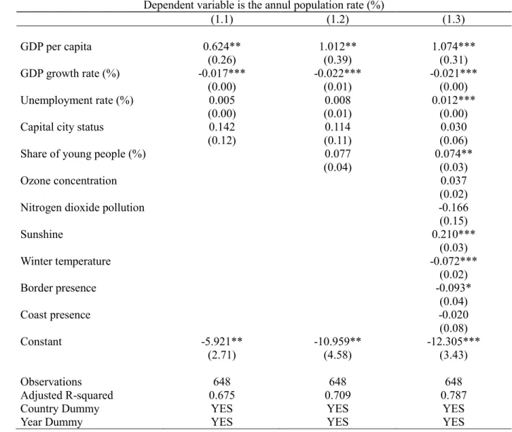
Based on the literature review, we identify potential urban migration determinants and construct a reference model to explain differences in metropolitan population growth rates through economic, sociodemographic and natural amenity-based conditions. Table 1 presents the model’s three-step derivation with each column including an additional set of explanatory variables and the last column representing the final specification.
First, Model 1.1 shows that economic conditions that represent regional wealth act as significant migration drivers. A higher standard of living, as measured by GDP per capita, positively correlates with population growth. This hints that within-EU differences in local economic incentives exist that motivate people to relocate, which is contrary to what we observe in the US. Surprisingly, GDP growth, which reflects a metropolitan’s economic expansion, is associated with lower levels of population growth. The relationship between unemployment rates or capital city status with the depended variable is not statistically significantly different from zero.
TABLE 1: Results of pooled OLS Regression: Reference Model
Dependent variable is the annul population rate (%)
(1.1) (1.2) (1.3)
GDP per capita 0.624** 1.012** 1.074***
(0.26) (0.39) (0.31)
GDP growth rate (%) -0.017*** -0.022*** -0.021***
(0.00) (0.01) (0.00)
Unemployment rate (%) 0.005 0.008 0.012***
(0.00) (0.01) (0.00)
Capital city status 0.142 0.114 0.030
(0.12) (0.11) (0.06)
Share of young people (%) 0.077 0.074**
(0.04) (0.03)
Ozone concentration 0.037
(0.02)
Nitrogen dioxide pollution -0.166
(0.15)
Sunshine 0.210***
(0.03)
Winter temperature -0.072***
(0.02)
Border presence -0.093*
(0.04)
Coast presence -0.020
(0.08)
Constant -5.921** -10.959** -12.305***
(2.71) (4.58) (3.43)
Observations 648 648 648
Adjusted R-squared 0.675 0.709 0.787
Country Dummy YES YES YES
Year Dummy YES YES YES
NOTES: Robust standard errors are in parentheses. ***, ** and * indicate significance at 1%, 5% and 10% level, respectively. All regressions include country and time dummies. Standard errors have been adjusted potential for serial correlation within metropolitan areas. Appendix Table B1 provides the exact definitions of all variables.
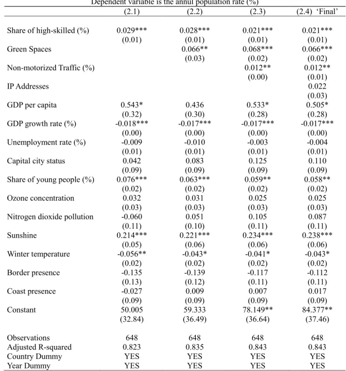
5.2. Pooled OLS Results and Discussion
TABLE 2: Results of Pooled OLS Regression: Smart Amenities
Dependent variable is the annul population rate (%)
(2.1) (2.2) (2.3) (2.4) ‘Final’
Share of high-skilled (%) 0.029*** 0.028*** 0.021*** 0.021***
(0.01) (0.01) (0.01) (0.01)
Green Spaces 0.066** 0.068*** 0.066***
(0.03) (0.02) (0.02)
Non-motorized Traffic (%) 0.012** 0.012**
(0.00) (0.01)
IP Addresses 0.022
(0.03)
GDP per capita 0.543* 0.436 0.533* 0.505*
(0.32) (0.30) (0.28) (0.28)
GDP growth rate (%) -0.018*** -0.017*** -0.017*** -0.017***
(0.00) (0.00) (0.00) (0.00)
Unemployment rate (%) -0.009 -0.010 -0.003 -0.004
(0.01) (0.01) (0.01) (0.01)
Capital city status 0.042 0.083 0.125 0.110
(0.09) (0.09) (0.09) (0.09)
Share of young people (%) 0.076*** 0.063*** 0.059** 0.058**
(0.02) (0.02) (0.02) (0.02)
Ozone concentration 0.032 0.031 0.025 0.025
(0.03) (0.03) (0.03) (0.03)
Nitrogen dioxide pollution -0.060 0.051 0.105 0.087
(0.11) (0.10) (0.11) (0.11)
Sunshine 0.214*** 0.221*** 0.234*** 0.238***
(0.05) (0.06) (0.06) (0.06)
Winter temperature -0.056** -0.043* -0.041* -0.043*
(0.02) (0.02) (0.02) (0.02)
Border presence -0.135 -0.139 -0.117 -0.112
(0.13) (0.12) (0.11) (0.11)
Coast presence -0.027 0.009 0.007 0.017
(0.09) (0.09) (0.09) (0.09)
Constant 50.005 59.333 78.149** 84.377**
(32.84) (36.49) (36.64) (37.46)
Observations 648 648 648 648
Adjusted R-squared 0.823 0.835 0.843 0.843
Country Dummy YES YES YES YES
Year Dummy YES YES YES YES
NOTES: Robust standard errors are in parentheses. ***, ** and * indicate significance at 1%, 5% and 10% level, respectively. All regressions include country and time dummies. Standard errors have been adjusted potential for serial correlation within metropolitan areas. Appendix Table B1 provides the exact definitions of all variables.
0.115% increase in the population growth rate. The direction of the observed effect is in line with Rodríguez-Pose and Ketterer (2012), who find a positive causal effect of human capital on urban migration rates. However, this variable needs to be treated cautiously due to potential endogeneity from worker’s self-selection. As argued by Cheshire and Magrini (2006), migrants have higher human capital endowments than non-migrants, which results in a composition effect. The level of human capital of the metropolitan area attracting additional households grows relative to that of its neighbors. Evidence from the US proposes that one third of the population growth induced by human capital accumulation results from improvements in urban QOL, such as growth of consumer services, and two thirds from increased productivity, such as localized knowledge spillovers (Shapiro, 2006).
The inclusion of urban recreation areas increases the explanatory power of our model from 0.823 to 0.835. A one percent increase in the amount of green spaces per capita is on average correlated with a 0.091% increase in the population growth rate. As green areas compete for land with commercial and residential usage we assume their presence increases local housing prices more directly than other amenities. The significant impact of their availability on urban attractiveness is a strong indicator for the perceived improvements in QOL that households expect from it. These improvements might arise from intangible benefitssuch as aesthetic value, social inclusion and the promotion of public health and safety (Takano et al., 2002; Maas et al., 2006). In a study of German cities, Buch et al. (2013) observe a similar effect, although at a different order of magnitude. Their analysis provides evidence that a one standard deviation increase in the share of total land area covered by green spaces generates a 0.524% – 1.127% increase in cities’ migration rate. It is likely that this discrepancy in the point estimates is partially generated by different specifications of the empirical model as well as by the use of alternative measures of population growth and measurement of green spaces variables. However, it might also indicate that Germans, who enjoy a comparatively high GDP per capita within Europe, place greater weight on non-economic factors in their location decisions. Additionally, this might be the case because income differentials within Germany are smaller than income differentials within the EU.
result in reduced housing costs.32
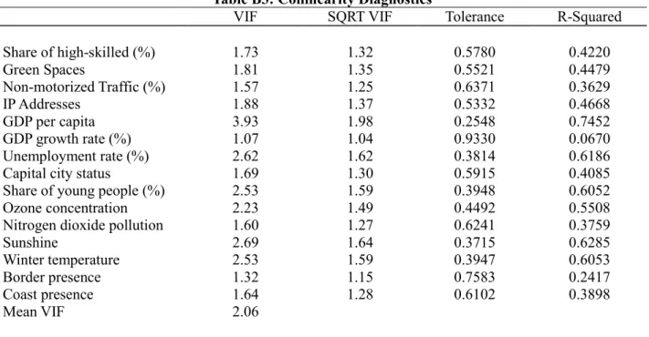
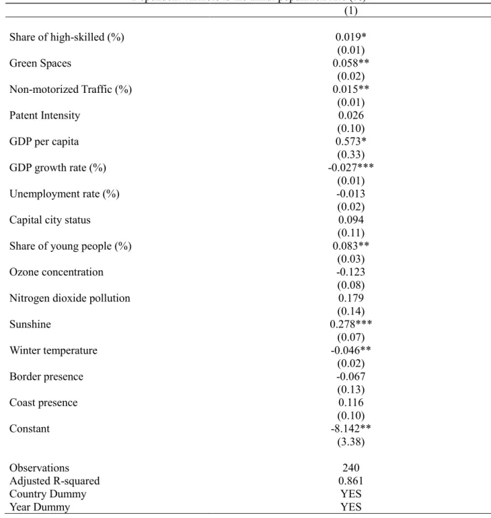
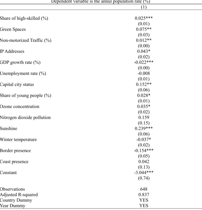
Surprisingly, the results in Table 2 do not indicate a statistically significant linear dependence of the mean of population growth on the amount of Internet Protocol (IP) addresses per capita. We would expect cities with better ICT infrastructure to attract population growth because they offer, inter alia, larger potential for innovation and entrepreneurial activities. The use of patent intensity as an alternative proxy for cities’ innovative capacity and level of technological adaption produces similar results.33 We suspect
multicollinearity to reduce the precision of these regressions as the correlation between GDP per capita and IP addresses per capita measures close to 0.56. Appendix Table B5 excludes GDP per capita and points towards a statistically significant, positive correlation between a metropolitan area’s population growth and their level of technological adaption. In Section 5.3., we discuss simultaneity concerns, which further motivate the exclusion of GDP per capita. Due to its superior goodness of fit, we prefer Model 2.4 to this alternative specification.
To test the preposition about the positive correlation between smart amenities and population growth further, we a perform Wald test on a linear combination of smart city coefficients as given by following null and alternative hypothesis:
𝐻0: 𝛽12+ 𝛽12+ 𝛽12+ 𝛽12≤ 0 (16)
𝐻𝐴: 𝛽12+ 𝛽12+ 𝛽12+ 𝛽12> 0 (17)
Based on the resulting one-sided p-value, we accept the alternative hypothesis at the 1% significance level. Overall, we conclude that our analysis of European metropolitan areas indicates a positive correlation
between population growth rates and the local presence of highly skilled individuals, recreational areas and infrastructure for non-motorized transport. Extending upon a reference model, which controls for differences in metropolitan population growth rates due to economic, sociodemographic and natural amenity-based conditions, we provide specific point estimates for the strength of this association. The adjusted R-squared reported in Table 2 is 0.843, which represents an increase above the reference model. Regarding the insignificant individual coefficient of IP addresses per capita, we propose an alternative specification with reduced multicollinearity, which reveals a significant and positive correlation between IP addresses and our dependent variable.
In the spatial equilibrium framework, these results suggest that cross-country migration flows within the EU react to perceived differentials in metropolitan area’s indirect utility levels. In line with
32 For further information on how land rents and housing prices depend on commuting costs in the open city model, see Duranton and Puga (2013).
Pose and Ketterer (2012), the significance of economic, sociodemographic and amenity-based migration drivers tends to support the existence of European amenity-based migration. In particular, the effect of human capital, non-motorized traffic and urban green spaces indicates that perceived utility differentials are partially generated by local differences in the endowments of smart amenities. Consequently, the application of Smart City development concepts might enhance the attractiveness of European metropolitan areas towards migrants. This contrasts with Cheshire and Magrini (2006), who argue that due to low factor mobility, cross-country migration flows in the EU are exclusively determined by differentials in economic conditions. Europeans appear to assign increasingly more weight to amenities in their location choice, which might be due to rising standards of living, ongoing economic integration or declining migration and information costs (Partridge, 2010).
Our results, however, are subject to theoretical and empirical shortcomings. Based on our empirical identification strategy alone we are not able to draw inferences about the causal relationship between population growth rates and the presence of smart amenities; it merely suggests a correlation. The true nature of this association might be that smart amenities are a determinant of migration flows, a reaction to migration flows, or both are caused by a third unobserved factor. For example, migration to high amenity cities might be a consequence of economic growth, which increases the demand for urban amenities, not of changes in the supply of amenities. Under the assumptions introduced in Section 3, migration flows are indicative of the existence of spatial utility differentials. However, these assumptions are simplistic. In particular, we model households with homogeneous preferences, which only allows one-directional migration flows to occur. In reality, preferences are likely to be very heterogeneous and context dependent as they might arise from households’ incomes, life cycle and cultural values. Our framework neglects the information resulting from bi-directional migration flows, as these cancel each other out in the net migration balance. Further, as outlined in Section 2, the assumption of (perfect) mobility might be violated in the EU context. Households face pecuniary and non-pecuniary moving costs, which prohibit them from acting upon relatively small potential utility gains from migration. Thus, migration rates might not fully reveal the reprehensive households’ preferences about a city’s attractiveness.
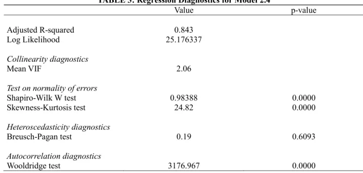
5.3. Tests of Model Specification and Robustness
Shapiro-Wilk W test for normality and the Skewness-Kurtosis test lead us to reject the null hypothesis of normally distributed residuals. We attempt to correct for this misspecification using Huber-White robust standard errors in all models. Further, the Breusch-Pagan test for heteroscedasticity indicates homogeneity of variance. Visual inspection of the residuals supports this proposition. Finally, the Wooldridge test suggests the presence of first-order autocorrelation within the observations of each metropolitan area (Wooldridge, 2002). Serial correlation might indicate the presence of migrant networks, which facilitate future migration. Other European migration studies account for this by including an autoregressive term of population growth rates or net migration rates in their model specification (Rodríguez-Pose and Ketterer, 2012). We cluster standard errors at the metropolitan level to adjust our estimates for this lack of independence.
TABLE 3: Regression Diagnostics for Model 2.4
Value p-value
Adjusted R-squared 0.843
Log Likelihood 25.176337
Collinearity diagnostics
Mean VIF 2.06
Test on normality of errors
Shapiro-Wilk W test 0.98388 0.0000
Skewness-Kurtosis test 24.82 0.0000
Heteroscedasticity diagnostics
Breusch-Pagan test 0.19 0.6093
Autocorrelation diagnostics
Wooldridge test 3176.967 0.0000
of this specification. While the coefficient of IP addresses per capita turns significant, all other smart amenities are almost unchanged. Further, we utilize predetermined variables as an internal instrument to reduce simultaneity bias. However, external instrumental variables would be a valuable addition to this thesis. Unobserved time-invariant heterogeneity of metropolitan areas might introduce omitted variable bias to the pooled OLS regression. Municipal efficiency and other important unobserved city characteristics might influence urban population growth rates. Consequently, we estimate regression (x) under the inclusion of city-specific fixed effects. The FE model, however, performs significantly worse than the pooled OLS version. In particular, its goodness of fit as measured by the adjusted R-squared is 0.576. This leads us to reject the FE results in favor of the pooled OLS results. While we identify and partially address the main sources of endogeneity in our model, we urge to consider the regression results in Table 2 with caution.
An additional caveat of our analysis is the lack of spatial analysis due to the lack of geographic location data. In the study of urban amenities, there are several potential sources of spatial dependence. For example, the diffusion of urban development best practices from one metropolitan area might affect neighboring regions stronger than more distanced ones. In addition, relocating households face migration costs that depend on the distance between their origin and their destination. As a result, the error terms across different FURs might be correlated (spatial error) or the population growth in a FUR might be affected by the explanatory variables of other FURs (spatial lag). This would violate the OLS assumptions and lead to biased estimates. In their analysis of a comparable dataset of European metropolitan areas, Cheshire and Magrini (2006) show that spatial dependences do not significantly bias the results of pooled OLS regressions on urban population growth rates. Nonetheless, it would be sensible to test our specification for the degree of spatial dependence using information on the geographic distances between the individual observational units and, if necessary, to control for inconsistencies through a spatial lag or error model.
Finally, while we conducted the compilation and aggregation of data sources as diligently as possible, we notice that the mismatch of spatial units potentially introduces biases related to the presence of different demographic groups in the core city and its commuting zone, the unequal migration pull of these territories and the local impact of urban planning activities.