Banco Comercial Português : equity valuation

(1)

Católica Lisbon School of Business & Economics

Banco Comercial

Português

Equity Valuation

Author: João Miguel Magalhães da Silva Pessanha, nr. 152110304

Advisor: Prof. José Carlos Tudela Martins

Abstract

Many financial analysts across the world try to understand on a daily basis if the price of a specific stock will go up or down. They combine all the existent theory regarding valuation with their practical experience and insight as support to strengthen their arguments over the fair value they recommend/’sell’. Similarly, my objective in this dissertation was to present different valuation methodologies and achieve reliable and as accurate as possible the share fair value of Banco Comercial Português, also known as Millennium BCP. The year-end 2013 price target yielded by my valuation model was 0,157 Euros per share, representing a potential return to the investor of 65,2% - BUY recommendation. I also performed a sensitivity matrix, showing how the implicit price target changes due to small changes in key variables of the model. Furthermore, a comparison with an equity research of a leading investment bank was done, mainly focusing on methodologies followed and results obtained.

Dissertation submitted in partial fulfillment of requirements for the degree of MSc in Business Administration, at the Universidade Católica

(2)

2 CONTENTS I. PREFACE ... 7 1. INTRODUCTION ... 8 2. LITERATURE REVIEW ... 10 2.1 Overview ... 10

2.2 The role of valuation ... 10

2.3 Choosing a valuation model ... 11

2.4 Main valuation models ... 12

2.4.1 Asset-Based Valuation ... 13

2.4.2 Discounted Cash Flow Models ... 13

2.4.2.1 Different models on DCF approach ... 14

2.4.2.1.1 Free Cash Flow to the Firm (FCFF) valuation ... 15

2.4.2.1.2 Adjusted Present Value (APV) valuation... 16

2.4.2.1.2.1 Value of the unlevered Firm ... 16

2.4.2.1.2.2 Present Value of Interest Tax Shields ... 17

2.4.2.1.2.3 Expected Bankruptcy Costs... 18

2.4.2.1.3 Capital Cash Flow (CCF) Model ... 19

2.4.2.1.4 Economic Value Added (EVA) valuation ... 20

2.4.2.1.5 Dividend Discount Model (DDM) ... 21

2.4.2.1.6 Free Cash Flow to the Equity (FCFE) valuation ... 23

2.4.2.1.7 Dynamic ROE – DuPont Approach ... 24

2.4.2.1.8 Net Asset Value Approach ... 25

2.4.2.2 Key inputs of DCF models... 26

2.4.2.2.1 Cost of Equity (RE) (CoE) ... 26

2.4.2.2.1.1 Risk-free rate (Rf) ... 27

2.4.2.2.1.2 Beta (β) ... 27

2.4.2.2.1.3 Market Risk Premium (Rm - Rf) ... 29

2.4.2.2.2 Cost of Debt (RD) ... 29

2.4.2.2.3 Weighted Average Cost of Capital (WACC) ... 30

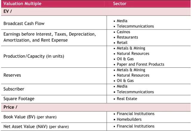
2.4.3 Relative Valuation - Multiples ... 30

2.4.3.1 Types of Multiples... 31

2.4.4 Contingent Claim Valuation Models ... 33

2.5 Valuing Financial Institutions ... 33

2.6 Cross-Border Valuation ... 35

3. BANCO COMERCIAL PORTUGUÊS (Millennium BCP) ... 37

3.1 Company Presentation ... 37

3.2 Shareholder Structure ... 39

3.3 Share Price Performance ... 40

3.4 Financial Performance ... 41

3.4.1 Profitability ... 41

(3)

3 3.4.3 Solvency ... 43 3.4.4 Liquidity ... 44 3.4.4.1 External Funding ... 45 3.4.5 Asset Quality ... 46 3.4.6 Ratings ... 47 3.5 Recapitalization Plan (2012) ... 48 3.6 Strategic Program (2013-2017) ... 50 4. SECTOR ANALYSIS ... 51 4.1 Banking Sector ... 51 4.1.1 Portugal ... 51 4.1.2 Poland ... 53 4.1.3 Angola ... 56 4.1.4 Mozambique ... 58 4.2 Regulatory Framework ... 60 5. VALUATION METHODOLOGY ... 62

5.1 Exclusion of other valuation models ... 62

6. ASSUMPTIONS... 64

6.1 Related with the macroeconomic indicators ... 64

6.2 Related with the Cost of Equity (CoE) ... 64

6.2.1 Portugal and Poland ... 65

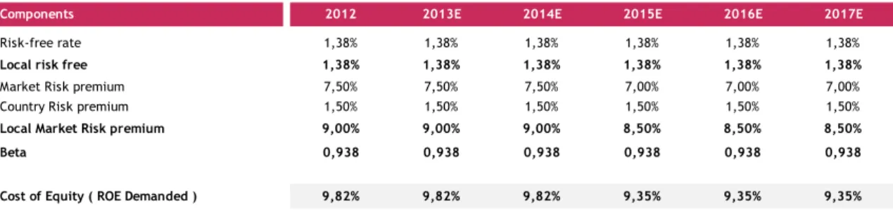
6.2.2 Angola and Mozambique ... 66

6.2.3 Greece ... 68

7. VALUATION OF MILLENNIUM BCP ... 69

7.1 Portugal ... 69

7.1.1 Selected volume figures ... 69

7.1.2 Selected results ... 71

7.2 Poland ... 74

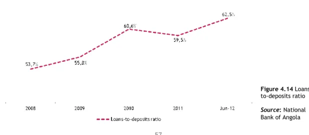
7.3 Angola ... 76

7.4 Mozambique ... 79

7.5 Greece ... 81

8. VALUATION RESULTS ... 84

8.1 Net Asset Value (NAV) Approach ... 84

8.2 Sensitivity analysis ... 88

(4)

4

8.4 Valuation comparison with BBVA Research ... 93 9. CONCLUSIONS ... 97 10. APPENDIXES ... 99

(5)

5

Hope for profits after the

RE-capitalization/structure

FY13 Reccomendation

BUY

Price Target Eur 0,157

In the end of the FY12, Millennium BCP posted a consolidated net loss of Eur -1.220 million, extremely penalized by impairment for estimated losses and results associated with the Greek operation in the amount of Eur -694 million. After the recapitalization operations, the issuance of Contingent Convertibles (‘CoCos’) (Eur 3.000 million) in June and the rights issue guaranteed by the Portuguese State (Eur 500 million) in September, Core Tier 1 reached in the end of the year 12,4% according to Bank of Portugal. The deleveraging process continued in 2012, with a decrease of Eur 5.246 million on the commercial gap and the improvement of the loans-to-deposits ratio to 129%.

Slow recovery of profitability in Portugal

The domestic operation will be under pressure until 2016. The ‘CoCos’ interest payments (avg. interest rate of 9,15%) and the high level of loans impairment contribute for net losses until 2015. The recovery of profitability in Portugal will come back in 2016, following the net interest income improvement, the decrease of the cost of risk and the cost cutting initiatives.

Foreign operations continue growing. Greece for sale.

The improvement of the banking income and the strict control of costs will support the good performance of the Polish operation. The increasing penetration of the banking activity in Angola and Mozambique will allow continue growing in these markets. Initiated discussions to sell the Greek operation. Potential bidder is Piraeus Bank.

Expected upside: 65,2%

Bloomberg

BCP PL Reuters BCP.LS Share price: Eur 0,095 (closing price as 28-Mar-13)

Market Cap. Eur 1.872m Nr. of shares 19.707m

Share price performance (July11 – March13)

Market performance (YTD %)

Historical financial highlights (2010-2012)

Sources: Bloomberg, BCP, own estimates

Millions of Euros 2012 2013 E 2014 E 2015 E 2016 E 2017 E

Net interest income 493 537 607 720 843 1.077

Net operating revenues 1.253 1.083 1.206 1.384 1.533 1.785

Operating costs 872 704 732 780 800 854 Net income (669) (452) (248) (58) 117 333 ROE -15,3% -10,4% -5,6% -1,3% 2,4% 6,8% NIM 0,8% 0,9% 1,0% 1,1% 1,3% 1,6% C/I 66,3% 61,3% 57,3% 53,3% 49,3% 45,3% Cost-of-Risk (bps) 179,3 165,7 134,5 109,4 88,9 73,0 Loans-to-deposits 152,1% 152,1% 152,1% 152,1% 152,1% 152,1%

Overdue loans / Total loans 6,5% 5,9% 5,0% 4,2% 3,6% 3,0%

Total impairment / Overdue loans 89,3% 89,3% 89,3% 89,3% 89,3% 89,3%

Millions of Euros 2012 2013 E 2014 E 2015 E 2016 E 2017 E

Net interest income 492 569 631 697 766 840

Net operating revenues 863 958 1.049 1.149 1.258 1.375

Operating costs 533 564 616 673 732 793

Net income (30) 7 72 145 196 265

Net income (w/out Greece) 237 270 300 334 346 383

-20% -15% -10% -5% 0% 5% 10% 15% 20% 25% 30%

Millions of Euros 31 Dec. 10 31 Dec. 11 31 Dec. 12

ROE 9,8% -22,0% -35,4% ROA 0,3% -0,9% -1,3% NIM 1,68% 1,74% 1,20% C/I 54,1% 58,4% 66,6% Core Tier I 6,7% 9,3% 12,4% Loans-to-deposits 163,6% 144,8% 129,0%

Overdue loans / Loans 3,0% 4,5% 6,2%

Immpairment / Overdue loans 109,4% 109,1% 101,6%

Total assets 98.547 93.482 89.744

Loans to customers (net) 73.905 68.046 62.618

Customer deposits 45.609 47.516 49.390

NII 1.516 1.580 1.023

Net operating revenues 2.902 2.570 2.180

Operating costs 1.543 1.634 1.459

Net income 345 (848) (1.220)

Branches 1.744 1.722 1.699

Employees 21.370 21.508 20.365

(6)

6

Valuation FY13

Facing the specifications and risks of each market where Millennium BCP operates, I develop a Sum of Parts (SoP) approach based on NAV model, valuing each geographic segment separately and then summing up the BCP’s value in Portugal to the international value of the Bank. For this purpose, I use historical individual financial statements (until December 2012) to forecast the correspondent components for the next five years (until December 2017), and I apply an individual cost of equity that incorporates the risks associated to each market. I assume a Sustainable ROE which reflects the Banks’ ability to deliver profitability under stable market conditions in the long-term. Furthermore, I consider the current pension fund shortfall that must be adjusted to the BCP’s final valuation.

Valuation comparison with trading ‘peers’ Sources: Bloomberg, own estimates

Analyst: João Miguel Magalhães da Silva Pessanha

Millions of Euros Equity Value 13E Net income 13E Forecasted ROE 13E CoE 13E Sustainable

ROE G P/NAV Valuation

% of Capital held Attributable Per share % Valuation Implied P/E BCP GROUP 6.394 (445) -7,0% 0,6x 4.149 3.279 0,17 106,0% -7,4x Millennium BCP - Portugal 4.330 (452) -10,4% 15,8% 6,8% 0,9% 0,4x 1.717 100% 1.717 0,09 55,5% -3,8x

Bank Millennium - Poland 1.238 128 10,4% 9,8% 11,7% 1,8% 1,2x 1.524 65,5% 998 0,05 32,3% 7,8x

Banco Millennium - Angola 247 39 15,7% 14,5% 15,7% 2,7% 1,1x 271 52,7% 143 0,01 4,6% 3,7x

Millennium bim - Mozambique 390 103 26,4% 14,6% 21,7% 3,9% 1,7x 649 66,7% 433 0,02 14,0% 4,2x

Millennium Bank - Greece 188 (263) -139,5% 28,6% 0,0% 1,8% -0,1x (12) 100% (12) 0,00 -0,4% 0,0x

# Number of shares (13E) (millions) 19.707

Adjustments (185) (185) -0,01 -6,0%

Pension Fund shortfall (185) (185) -0,01 -6,0%

VALUATION (13E) 3.093 0,157 100,0%

Lx closing price (28.03.2013) 0,095 Income (e.g. Dividends) 0,000 Expected Holding Period Return (HPR) - Dec13 65,235%

0,0x 0,1x 0,2x 0,3x 0,4x 0,5x 0,6x 0,7x 0,8x 0,9x 0 10.000 20.000 30.000 40.000 50.000 60.000 70.000 80.000 90.000 P/ N A V

Total assets (m Eur)

0,0x 0,2x 0,4x 0,6x 0,8x 1,0x 1,2x 1,4x 1,6x 1,8x 2,0x 0 10.000 20.000 30.000 40.000 50.000 P/ N A V

Total assets (m Eur)

-0,2x 0,0x 0,2x 0,4x 0,6x 0,8x 1,0x 1,2x 1,4x 1,6x 0 10.000 20.000 30.000 40.000 50.000 60.000 70.000 80.000 P /N A V

(7)

7

I. PREFACE

As a Mergers & Acquisitions (M&A) analyst, the understanding and creation of valuation models will be part of my work. Therefore, this dissertation was an opportunity to improve my technical skills and expertise in valuation modeling, especially for financial services companies. I chose to value Millennium BCP’s share price due to the incredible challenges posed in its valuation, even more during the current economic environment in Europe which has been having a tremendously unpredictable impact on the European banking system. I would like to express my thankfulness to Professor José Carlos Tudela Martins for the constant availability and helpful feedback throughout the accomplishment of this dissertation.

I would like to appreciate the support provided by Millennium BCP’s Investor Relations Officer, Dr. Sofia Raposo, in terms of information and data collection. I am also very grateful to her for the several meetings we had and all the explanations provided.

On PricewaterhouseCoopers (‘PwC’), I am grateful to the Mergers & Acquisitions team, where I currently work, for the support, advice and understanding - Dr. Cidália Santos, Dr. Alexandra Viana, Dr. Narciso Melo, Dr. Gonçalo Adrião and Dr. José Nunes Pereira. I would also like to thank the knowledge transmitted by the Valuation & Strategy team of PwC.

Finally, I would to express my gratitude to my father by the constant support provided during my master degree, as well as the critical advice throughout the development of my thesis; and to my family and girlfriend, Isabel, by all support given.

(8)

8

1. INTRODUCTION

This dissertation aims to value the share price of Banco Comercial Português S.A. (“Millennium BPC”, “BCP”, “Bank”). Currently, BCP shares are listed in over 25 national and international stock market indexes, from which PSI-20 Index might be highlighted. Millennium BCP share is the most traded share in the Portuguese market, as it is the most liquid security on the domestic market.

Millennium BCP Group is the largest Portuguese private bank and the second bank when state-owned banks are considered, just behind Caixa Geral de Depósitos. According with the Annual Report of the Bank, it has total assets of 89.744 million Euros, loans and advances to customers (gross) of 66.861 million Euros and customer funds of 68.547 million Euros at 31 December 2012.

The Bank offers a wide variety of banking solutions and other financial services to its clients in Portugal and internationally, operating in Poland, Greece, Mozambique and Angola. It also has small operations in Romania and Switzerland.

Through the Net Asset Value (NAV) model, I value each core operation separately – Portugal, Poland, Angola, Mozambique and Greece. Then, I use the Sum of Parts (SoP) approach to reach the fair price per share of Millennium BCP for 2013, providing a buy/sell recommendation to readers. For this purpose, I use historical individual financial statements (until December 2012).

The structure of my thesis is the following:

In the ‘Literature Review’ (Section 2.), I explain the role of valuation by considering its practical scope in finance. I describe the different valuation models mostly used by financial practitioners, as well as the key inputs of each valuation model. Furthermore, I understand the implicit complexity in the approach of banking valuation.

A detailed company presentation is done in the ‘Banco Comercial Português’ (Section 3.). I describe Millennium BCP’s history, market position, shareholder structure and historical share price performance. Further, I analyze the financial performance of the Bank until December 2012, mainly concerning profitability, efficiency, solvency, liquidity, external funding, asset quality and ratings. I also describe the Bank’s recapitalization plan and the strategic program until 2017.

I provide a banking ‘Sector Analysis’ (Section 4.) in the core markets where Millennium BCP operates – Portugal, Poland, Angola and Mozambique (excluding Greece due to the fact that this geography is out of the Group’s strategic plan). Accordingly, I evaluate macroeconomic performance in the countries mentioned above, as well as their banking system historical profitability, asset quality, solvency and liquidity ratios.

(9)

9

In the ‘Valuation Methodology’ (Section 5.), I explain the reasons for choose Net Asset Value approach as my valuation model. Furthermore, I describe the reasons for exclude some models usually applicable to banking valuation.

I describe and explain the key ‘Assumptions’ (Section 6.), considered in the BCP’s valuation, related with macroeconomic forecasts and cost of equity.

In the ‘Valuation of BCP’ (Section 7.), I present the individual forecasts assumed and the implicit details for Balance Sheet and Income Statement of each geography – Portugal, Poland, Angola, Mozambique and Greece.

Finally, the ‘Valuation Results’ (Section 8.) yielded from my model are delivered and explained.

I also perform a sensitivity matrix, showing how the implicit price target changes due to small changes in key variables of the model, and compare the results of my valuation with the current trading multiples of comparable banks for each subsidiary.

Furthermore, I compare my model, in terms of assumptions and price target, with the equity research of a leading investment bank (Section 8.4.).

To finish, my ‘Conclusions’ (Section 9.) are expressed. Limitations/risks to fair value are also listed, mainly regarding the huge unpredictability of the ongoing restructuring process’s impact in Millennium BCP.

(10)

10

2. LITERATURE REVIEW 2.1 Overview

Valuation models have been evolving constantly since the recognition of their importance for strategic decisions in finance. Consequently, the existent literature about how to value a company is wealthy and very extensive. By taking into account the vast theoretical valuation metrics I will recognize the extent of each valuation model before comprehend which ones best fit on Millennium BCP valuation.

In this chapter I will explain the role of valuation by considering its scope in ‘finance world’. Then, I will describe the valuation models used by financial practitioners, discussing their advantages and disadvantages, as well as the key drivers of each valuation model.

Furthermore, I will understand which the main concerns that must be considered in the valuation of a financial service company, as Millennium BCP. Finally, I will select the valuation model which I will use for my valuation of this particular company.

2.2 The role of valuation

Koller et al. (2005) stated that “valuation is an age-old methodology in finance”. The same authors considered that “its intellectual origins lie in the present value method of capital budgeting and in the valuation approach developed by Professors Merton Miller and Franco Modigliani in their 1961 Journal of Business article entitle “Dividend Policy, Growth and the Valuation of Shares””.

Nowadays, as Damodaran (2002) argued, the relevance of valuation is reflected, mainly, in two financial areas, namely Corporate Finance (including Merger & Acquisition transactions) and Portfolio Management.

Valuation assumes a critical role as it supports strategic corporate finance decisions such as Mergers & Acquisitions, Privatizations, Private and Public Sales (IPOs), Dividend Policy, Leverage Buyouts and other investment opportunities or divestment processes. For this reason, the majority of investment banks and financial consultancy companies have specialized departments providing valuation services to their corporate clients, supporting the idea that an accurate valuation prepared by financial specialists is crucial to avoid taking bad decisions.

Concerning with Mergers & Acquisitions transactions, valuation plays a central part in the deal analysis. Damodaran (2002) stated that the bidding firm has to figure out the fair value for the target firm (including potential synergies) before making a bid, and the target firm has to determine a reasonable value for itself before deciding to accept or reject the offer.

In what concerns the other strategic corporate finance decisions presented above, if the objective is the maximization of firm value, the relationship between the financial decisions,

(11)

11

corporate strategy, and firm value has to be delineated. For Damodaran (2002), understanding this relationship through valuation methodologies is key to making value-increasing decisions.

Regarding Portfolio Management, the role that valuation plays is determined by the investor’s profile and philosophy. Whereas valuation is meaningless for a passive investor, the role of valuation for an active investor is substantial. For active investors, valuation provides fundamental information (growth prospects, risk profile, cash-flows, etc.) used to understand the future trend of the company’s stock price.

Fama (1970) argued that the market efficiency hypothesis lies on the assumption that stock prices at any time “fully reflect” all available information, therefore stock returns are unpredictable and follow a random walk. Considering this hypothesis, Damodaran (2006) recognized the importance of valuation methods in supporting investors to analyze whether and why market prices deviate from value, and how quickly they revert back.

For the reason stressed above, valuation is being a critical approach to support the stock selection decision for asset managers, traders and other investors. By taking into account the importance of valuation for capital markets players, research coverage has been increasingly centralized on companies’ valuation. Nowadays, equity research analysts perform valuations regularly in order to provide ‘buy’ and ‘sell’ recommendations to their clients, by comparing the intrinsic value of a stock against its value in the market.

Summing up, Damodaran (2006) considered that valuation is the “heart of finance”, being a prerequisite for making sensible strategic decisions and understanding how they affect the value of the company.

2.3 Choosing a valuation model

As Fernandez (2007) stated, for any financial practitioner involved in corporate finance, “understanding the mechanisms of company valuation is an indispensable requisite”. This is not only because of the importance of valuation but also because “the process of valuing the company and its business units helps identify sources of economic value creation and destruction within the company”. Furthermore, identifying the key drivers of the models used in valuation helps to understand the impact of such drivers on the estimated value of the company.

Having valuation the aforementioned role in finance, professionals in the field have to choose the models that best fit the company under analysis. Damodaran (2002) argued that “the problem in valuation is not there are not enough models to value a company, it is that there are too many”.

Nevertheless, as argued by Young et al. (1999), “All Roads Lead to Rome”, “every popular valuation model is no more than a different way of expressing the same underlying model”.

(12)

12

Under a practical perspective, this implies that if we use equivalent assumptions when we are valuing a company, we will obtain a similar outcome for the different methods used. As Damodaran (2002) stated, deciding what approach should be used can be a critical step when valuing a company. The decision whether to choose a simple model or a more complex and sophisticated one depends on several factors, some of which related to the business being valued and the precision that is required, but many of which related to the analysts and the information he has about the company being valued.

2.4 Main valuation models

Fernandez (2007) and Damodaran (2002) recognized similar classifications schemes for valuation models. In general terms, both authors considered that firms or assets can be valued by using one of four main types of valuation approaches: asset-based which aims determining the net value of the assets owned by the firm; discounted cash flow that computes the present value of future cash flows to arrive at a value of equity or the firm; relative valuation that values the firm based on performance and accounting measures of a group of comparable firms; and option pricing approaches that use contingent claim valuation. According with Damodaran (2002), within each of these approaches there are different models that can determine the final value of the company or asset under analysis. Below there are the main valuation models that can be used within the four different valuation approaches stressed previously:

Main Valuation Models

Asset-Based

Valuation Discounted Cash Flow Models Relative Valuation Contingent Claim Models

 Book value

 Adjusted Book value  Liquidation value  Substantial value

 Equity Valuation

 Dividend Discount Model (DDM)  Free Cash Flow to

the Equity (FCFE)  Dynamic ROE –

DuPont approach  Firm Valuation

 Free Cash Flow to the Firm (FCFF)  Adjusted Present

Value (APV)  Capital Cash Flow

 Economic Value Added (EVA)  Multiples  Price-Earnings ratio (P/E)  Price-book ratio (P/BV)  Price-sales ratio (P/Sales)  Enterprise value to EBITDA (EV/EBITDA)  Enterprise value to EBIT (EV/EBIT)  Enterprise value to sales (EV/Sales)  Enterprise value to Reserves (EV/Reserves) (among others)

 Black & Scholes and Binomial

 Option to delay

 Option to expand  Option to liquidate

Figure 2.1 Main Valuation Models

In the next sections, I will describe the models presented above as well as the key drivers of each valuation model. Since Millennium BCP is a financial institution, meaning that it has particular characteristics which I will explain later (Section 2.5), I will present also the main concerns in its valuation from using the different models discussed. Finally, I will briefly

(13)

13

expose the concerns of cross-border valuation, particularly in emerging markets, which represents (among other) what Damodaran (2010) called as the “dark side of valuation”.

2.4.1 Asset-Based Valuation

From Fernandez’s (2007) perspective, the asset-based valuation is based on the principle that a “company’s value lies basically in its balance sheet”. Given the stationary characteristic of the balance sheet, these type of valuation methodologies determine the value of the company from a static viewpoint which, therefore, does not take into account the company’s possible future evolution. Furthermore, these methods do not take into account changes in other factors that also affect the value of a company such as: macroeconomic conditions, regulatory environment, organizational structure, etc..

Damodaran (2006) argued that the value of a business can be considered as “the sum of the values of the individual assets owned by the business”. Nevertheless, he pointed out a limitation of this model by looking to the differences between a balance sheet at market values, which incorporates not only the existing investment but also the expected future investments and their profitability, and a balance sheet at accounting values, which only takes into account the investment realized. Consequently, models using book values, as the ones included in the asset-based valuation, will yield a lower value for the company than the models which the excess returns, that come from future growth, are incorporated.

By ignoring the critical factors stressed above, asset-based valuation methods can lead to misleading conclusions regarding the company’s value. The severity of these misleading conclusions is even bigger if the company being valued is an institution operating in financial sector, as it is Millennium BCP. The value of a bank is especially sensible to changes in regulatory environment. Consequently, the value of Millennium BCP can vary significantly as it is affected by regulatory changes required by national and international supervision entities, such as Bank of Portugal (BoP) and European Central Bank (ECB).

Given the absence of potential/future changes in regulatory environment and other important factors, asset-based models do not fit on Millennium BCP valuation. As a result, I think it is not appropriate to develop a formal asset-based valuation for Millennium BCP and therefore I will not prosecute a deepest analysis of each model within the valuation approach discussed.

2.4.2 Discounted Cash Flow Models

As it is stated by Rosenbaum and Pearl (2009), “discounted cash flow analysis (“DCF Models”) is a fundamental valuation methodology broadly used by investment bankers, corporate officers, university professors, investors and other financial professionals. It is premised on the principle that the value of a company, division, business, or collection of assets (“target”) can be derived from the present value of its projected free cash flows”. A company’s projected cash flows are “derived from a variety of assumptions about its expected financial

(14)

14

performance, including sales growth rates, profit margins, capital expenditures, and net working capital requirements”. As Damodaran (2006) argued, these projected cash flows should be “discounted at a rate that accurately reflects their riskiness”.

According to Fernandez (2007), the standard formula associated with the Discount Cash Flow Models is represented by:

[2.1] Intrinsic Value =

.…

RVn = Where,

CFi =Cash Flow generated by the firm in the period i

RVn = Residual Value of the firm in the year n

R = Appropriate discount rate for the cash flows’ risk

g = expected growth rate of cash flows after the explicit period

Furthermore, Rosenbaum and Pearl (2009) stated that the company’s cash flows are typically projected for a period of five years. Nevertheless, this period (usually defined as ‘Explicit Period’) may be longer depending on the company’s sector, stage of development, and the underlying predictability of its financial performance. Given the inherent difficulties in accurately projecting a company’s financial performance over an extended period of time (and through different economic cycles), the residual value is used to capture the remaining value of the target company, beyond the explicit period.

2.4.2.1 Different models on DCF approach

Under the Discounted Cash Flow approach there are distinct methods for valuing a company. Accordingly, the main DCF models can be classified as Equity vs Firm valuation and Absolute vs Residual Income valuation. As Damodaran (2002) argued, the different methods available should produce equivalent outcomes for the value of the ‘target’ company. As the assumptions about growth and leverage are consistent among the different DCF models used, the value of the company’s equity should be the same using the firm approach (where the value of the firm is computed and then the outstanding debt is subtracted) and the equity approach (where the value of the equity is directly computed).

The following table presents the different DCF models classifications:

Main DCF Models Absolute valuation Return based valuation

Firm valuation Free Cash Flow to the Firm

(FCFF)

Adjusted Present Value(APV)

Capital Cash Flow(CCF)

Economic Value Added(EVA)

Equity valuation Dividend Discount Model

(DDM)

Free Cash Flow to the

Equity(FCFE)

Dynamic ROE- DuPont

approach

(15)

15

As it will be explained in the following chapters, among the different DCF models classifications mentioned above, the expected cash flows and the discount rate will change. Damodaran (2002) stated that “the discount rate will be a function of the riskiness of the estimated cash flows, with higher rates for riskier cash flows and lower rates for safer cash flows”.

2.4.2.1.1 Free Cash Flow to the Firm (FCFF) valuation

As it is presented in Figure 2.2, FCFF valuation model allows us to estimate the value of the entire company, including debt. As Damodaran (2002) pointed out, “the value of the firm is obtained by discounting the Free Cash Flow to the Firm (FCFF) and the Residual Value (RV) at the after-tax Weighted Average Cost of Capital (WACC), which is the cost of the different components of financing used by the firm, weighted by their market value proportions”. The WACC and the RV assumptions typically have a substantial impact on the valuation final output.

According to Rosenbaum and Pearl (2009), the FCFF valuation should follow the following steps:

Step I. Study the target and determine key performance drivers

Step II. Project Free Cash Flows to the Firm (FCFF)

Step III. Calculate after-tax Weighted Average Cost of Capital (WACC)

Step IV. Determine the Residual Value (RV)

Step V. Calculate the Present Value and estimate valuation Figure 2.3 Free Cash Flow to the Firm (FCFF) valuation steps

The focus of this valuation method is on the cash generation. Accordingly, Rosenbaum and Pearl (2009) defined the FCFF as “the cash generated by the company after paying all cash operating expenses and the associated taxes, as well as, the funding of Capital Expenditures (CAPEX) and Working Capital, but prior to the payment of any interest expense”. Therefore, FCFF is independent of capital structure as it represents the cash available to all capital providers (both debt and equity holders).

Fernandez (2007) considered that the FCFF is computed by the following formula:

Earnings Before Interest and Taxes (EBIT)

Less: Taxes paid on EBIT (at the effective tax rate)

Earnings Before Interest After Taxes (EBIAT)

Plus: Depreciation & Amortization Less: Capital Expenditures

Less: Increase/Decrease in Net Working Capital (∆ in NWC)

Free Cash Flow to the Firm

Figure 2.4 Free Cash Flow to the Firm Calculation

The enterprise value (EV) of the target company is estimated by summing up the discounted Free Cash Flows to the Firm and the Terminal Value, as it is indicated below:

[2.2] EV =

.…

TVn =

(16)

16 Where,

FCFFi =Free Cash Flow to the Firm in the period i

TVn = Terminal Value of the firm in the year n

WACC = Weighted Average Cost of Capital (after-tax) g = expected growth rate after the explicit period

2.4.2.1.2 Adjusted Present Value (APV) valuation

The APV valuation model indicates that the basis for the firm’s value is the unlevered scenario, when the firm is entirely financed with equity. As debt is introduced on the firm’s balance sheet, the APV model considers the net effect on value by taking into account both the benefits and the costs of borrowing. In general terms, Damodaran (2006) pointed out that debt usage to fund the company’s operations creates tax benefits (because interest expenses are tax deductible) and increases the expected bankruptcy costs (because the increase of the bankruptcy risk):

Accordingly, Damodaran (2006) and Fernandez (2007) argued that the enterprise value (EV) of the target company is estimated by summing up the value the unlevered firm and the effects of using debt as a source of financing:

[2.3] EV = Vunlevered + PVITS – PVE(BC)

Where,

Vunlevered =Value of the company unlevered

PVITS = Present Value of Interest Tax Shields

PVE(BC) = Present Value of the expected Bankruptcy Costs

By considering the formula presented above, Damodaran (2002) considered the APV valuation as a three-step process. First, the value of the unlevered firm is estimated. Secondly, the present value of the interest tax savings generated by borrowing a given amount of money is calculated. Finally, the expected bankruptcy costs for the firm’s debt level are evaluated.

2.4.2.1.2.1 Value of the unlevered Firm

The first step in the APV approach is the estimation of the value of the unlevered firm. This

can be easily done, by using the same formula [2.2] of the FCFF valuation model. By

definition, an unlevered firm is a firm which is entirely equity financed. Consequently, the WACC will be equal to the cost of equity when the company has no debt (known as unlevered cost of equity), which results on the formula presented below:

[2.4] EV =

.…

TVn = Where,

FCFFi =Free Cash Flow to the Firm in the period i

RU = unlevered Cost of Equity

(17)

17

2.4.2.1.2.2 Present Value of Interest Tax Shields

The second step in the APV approach is the calculation of expected tax benefit from using a certain level of debt as source of financing.

Modigliani and Miller (1963) showed that a firm paying taxes on income may lower the tax amount by resorting to debt financing if interest payments are tax deductible. These savings are called tax shields because debt financing shields income from taxes to some extent. Even so, the fundamentals of the interest tax shields valuation have been discussed by several authors since almost half a century.

Modigliani and Miller (1963) argued that the tax benefit is a function of the tax rate and interest payments of the firm and is discounted at the cost of debt. This point of view considers the tax shields as a perpetuity, assuming that the marginal tax rate and the cost of debt stay constant over time. Accordingly, the Present Value of Interest Tax Shields is given by the following formula:

[2.5] PVITS =

= D * tc Where,

PVITS =Present Value of Interest Tax Shields

D= Value of Debt (subject to interest payments)

RD = Cost of Debt (required rate of return by debtholders)

tc = Marginal corporate tax rate

Further literature has shown similar or different perspectives concerning the estimation of the tax benefits from debt usage proposed by Modigliani and Miller (1963).

Myers (1974), the pioneer of the APV approach, followed the roots proposed by Modigliani and Miller (1963). Therefore, Myers (1974) proposed calculating the value of tax shields by discounting the tax savings at the cost of debt. The argument is that the risk of the tax savings arising from the use of debt is the same as the risk of the debt. Then, according to Myers (1974) the present value of the interest tax shields should be valued by the following growing perpetuity formula:

[2.6] PVITS =

Miles and Ezzell (1980) proposed a different approach for the computation of the interest tax shields. Despite the same fundamental basis of the Modigliani and Miller (1963) point of view, Miles and Ezzell (1980) argued that the correct discount rate for the tax savings of a company with a fixed target debt ratio (D/VL at market values) is the cost of debt (RD) in the first year,

(18)

18

Consequently, the authors considered that the present value of interest tax shields follows a growing perpetuity, as it is indicated by the formula below:

[2.7] PVITS =

Later, Harris and Pringle (1985) proposed that the present value of the interest tax shields should be calculated by discounting the tax saving at the required rate of return on assets, which is equal to the unlevered cost of equity. The argument presented by Harris and Pringle (1985) is that the interest tax shields have the same systematic risk as the firm’s underlying cash flows and, therefore, should be discounted at the required return to assets. Hence, according to the authors, the value of the tax shield is given by:

[2.8] PVITS =

From the extensive literature about the estimation of the tax shields, it is not possible to reach an incontestable conclusion. Therefore, the tax savings calculation should be made according to the characteristics of the debt level (fixed or variable) and the characteristics of the company/business itself.

2.4.2.1.2.3 Expected Bankruptcy Costs

The third step of the APV model is to evaluate the effect of the debt usage on the default risk of the firm and on the expected bankruptcy costs. According with Damodaran (2002), the present value of the expected bankruptcy costs is estimated by the formula presented below:

[2.9] PVE(BC) = Probability of bankruptcy * PV of Bankruptcy Costs

Nonetheless, Damodaran (2002) stressed that this process poses the most significant estimation problems, since neither the probability of bankruptcy nor the bankruptcy costs can be estimated directly.

Damodaran (2001) argued that the probability of bankruptcy is the likelihood that the firm’s cash flows will be insufficient to meet its promised debt obligations, either interest or principal. Considering this definition, the probability of bankruptcy is a function of:

1st _{Size of Operating Cash Flows relatively to the size of the Debt Obligations}

2nd _{Variance in Operating Cash Flows}

Damodaran (2002) discussed three main methods to estimate the probability of bankruptcy. The first one is computing a probit analysis (stress tests, multiple scenarios test and other statistical approaches) taking into consideration the characteristics of the firm associated to different debt levels. The second way to compute the probability of bankruptcy is estimating a bond rating and uses the empirical estimates of default probabilities for the correspondent

(19)

19

rating. Finally, the probability of bankruptcy can be derived by reverse engineering (i.e. backing out the probability from the prices of corporate bonds issued by the firm).

The most critical and demanding part in estimating the present value of the expected bankruptcy costs is quantifying the costs associated to the bankruptcy. Considering Damodaran (2001), these costs can be classified into direct and indirect. The direct costs of bankruptcy are the costs incurred at the time of the bankruptcy and can be easily estimated. These costs are mainly administrative and legal expenses related to accountants’ and lawyers’ fees. In the other hand, the indirect costs of bankruptcy may be substantial relatively to the firm’s value. The indirect costs are categorized as the costs associated with the debt usage and the increasing default risk that arises prior to the bankruptcy. Accordingly, the indirect costs translate the customers’ and suppliers’ perception that the firm is financially deteriorating. For customers’ point of view, they may stop buying the product or service out of fear that the company will go out of the business. Further, as the debt level increases, company’s suppliers will demand stricter terms to protect themselves against the probability of default. Damodaran (2001) considered that the severity of these and other indirect costs (not mentioned) depends on the company’s business and on the products and services characteristics (durability, quality, maintenance, complementarity with other products or services, etc.). Despite their significant impact on company valuation, the indirect costs are very difficult to be measured.

2.4.2.1.3 Capital Cash Flow (CCF) Model

Ruback (2000) introduced the Capital Cash Flow model as a different way of valuing companies using the same assumptions and approach as the Free Cash Flow valuation model

(Section 2.4.2.1.1). Despite algebraically equivalent to the FCFF model, the CCF model includes

all of the cash available to capital providers, including the interest tax shields. In other words, Capital Cash Flows are equal to the Free Cash Flows plus the interest tax shields. Because the interest tax shields are included in the cash flows, the appropriate discount rate is before-tax and corresponds to the riskiness of the cash flows. As Ruback (2000) argued, the main advantage of the CCF valuation model is its simplicity either when the company has a fixed target debt ratio or when the debt ratio changes over time.

Ruback (2000) considered that the CCF is computed by the following formula:

Earnings Before Interest and Taxes (EBIT)

Less: Taxes paid on EBIT (at the effective tax rate)

Earnings Before Interest After Taxes (EBIAT)

Less: Increase/Decrease in Net Working Capital (∆ in NWC)

Free Cash Flow to the Firm

Plus: Interest Tax Shields

Capital Cash Flow

(20)

20

Then, the enterprise value (EV) of the target company is estimated by summing up the discounted Capital Cash Flows and the Terminal Value, as it is indicated below:

[2.10] EV =

.…

TVn = Where,

CCFi =Capital Cash Flow in the period i

WACC = Weighted Average Cost of Capital (pre-tax) g = expected growth rate after the explicit period

As it was stressed early, Capital Cash Flow method and the Free Cash Flow method are equivalent because they make the same assumptions about cash flows, capital structure, and taxes. Therefore, Ruback (2000) argued that both models should give identical outcomes. The choice between the two methods is only dependent on their ease of use, mainly concerning to the complexity of applying each method on the target company.

2.4.2.1.4 Economic Value Added (EVA) valuation

Koller et al. (2005) considered that despite the greater popularity of the methods presented

above (Sections 2.4.2.1.1/.2/.3), among financial professionals, academics and other

practitioners, they provide little insight into the company’s performance. In other hand, Economic Value Added (EVA) valuation highlights how and when the company creates value. As Damodaran (2006) stated, EVA model has its roots in capital budgeting and the net present value rule. The EVA measures the “excess return” of a project (including all future cash flows) against its capital needs. By considering this difference, the model measures the surplus value created by an investment or a portfolio of investments.

Conceptually, EVA is computed through main three inputs: the return on capital earned on investments, the cost of capital for those investments and the capital invested in them. The formula to estimate EVA is presented below:

[2.11] EVA = Invested Capital * (ROIC – WACC)

Since ROIC equals NOPLAT divided by invested capital, the formula can be rewrite as follows: [2.12] EVA = NOPLAT - (Invested Capital * WACC)

Where,

EVA=Economic Value Added

NOPLAT= Net Operating Profit Less Adjusted Taxes

WACC = Weighted Average Cost of Capital ROIC = Return on Invested Capital

(21)

21

Damodaran (2002) presented EVA model as a simple extension of the net present value rule. For this reason, investing in projects with positive net present value will increase the value of the firm, while investing in projects with negative net present value will reduce value. According with Damodaran (2006), the value of the firm can be estimated by summing up three components: the capital invested in assets in place, the present value of the economic value added by these assets, and the expected present value of the economic value that will be added by future investments.

Then, the enterprise value (EV) of the target company is estimated by the following formula: [2.13] EV = Capital Investedassets in place +

+

2.4.2.1.5 Dividend Discount Model (DDM)

As it is presented in the Figure 2.2, DDM measures only the equity value of the firm. As Damodaran (2002) stated, the rationale for the model lies again in the present value rule, meaning that the value of the company’s equity is “the present value of the expected future dividends", discounted at a rate appropriate to the riskiness of the dividends payment.

According with the definition presented by Damodaran (2002) and Fernandez (2007), the

future cash flows expected by the equity investors generally arise from two sources1_:

dividends during the holding period and the expected price at the end of the holding period (comparing with the initial price). Since the stock price is itself determined by future dividends, the only source of cash flows from the equity, which is considered by the model, is the dividends.

Concerning the discount rate for the model, it is determined by the riskiness of the stock returns, which is measured by the cost of equity. The cost of equity can be estimated according with several methods. Nevertheless, it is usually estimated using the capital-asset pricing model (CAPM), as it will be presented later (Section 2.4.2.2.1).

Fernandez (2007) argued that for a company which the investor is expecting dividends to grow at a constant rate indefinitely, the value of the equity can be easily estimated by using the Gordon Growth Model, as follows below:

[2.14] Equity Value = Where,

E (Dividends1)=Expected Dividends next year

RE = Cost of Equity

1

Other sources are share buy-backs and subscription rights. However, in the latter, when capital increase takes place trough a subscription of rights, the shares’ price falls by an amount approximately equal to the right’s value, meaning that the equity investors do not get a capital return.

(22)

22 g = growth rate in dividends forever

According with Damodaran (2002), despite “the Gordon Model provide a simple approach to valuing equity, its use is limited to firms that have no growing (assuming g equals to zero) or to firms that are growing at a stable growth rate”. The Gordon Models is also extremely sensitive to the growth rate defined by the analyst. When incorrectly defined, it can yield misleading or even absurd results.

For companies which the growth rate is unstable and the dividends paid to equityholders change over the time, more complex models should be used. Damodaran (2002) proposed the two-stage and the three-stage Dividend Discount Models to capture the changes in the growth rate and in the dividends value paid. However, these models require a much larger number of inputs, which may lead us to misleading outcomes when inconsistent.

When a reliable forecast about the dividends is made, the equity value can be estimated according with the formula presented below:

[2.15] Equity Value =

.…

TVn = Where,

E (Divi)=Expected Dividends in the period i

TVn = Terminal Value of the equity in the year n

RE = Cost of Equity

g = expected growth rate after the explicit period

One of the most important drawbacks of the DDM arises when the value creation is not implicit in the payout policy. As Damodaran (2006) pointed out there are “firms paying far more in dividends than they have available in cash flows, often funding the difference with new debt or equity issues”. In these particular companies, using the DDM will generate valuation results that are too optimistic, assuming that firms can continue to draw on external funding to meet the dividend deficits in the long-run. Other critic made to the DDM is when the companies pay no dividends. In spite of Damodaran (2006) defended that firms paying no dividends currently, can still be valued based upon dividends that they are expected to pay out in the future, some practitioners and financial professionals argue that, in this case, the model requires several assumptions regarding the future dividend policy, which can lead to inconsistent valuation outcomes.

Notwithstanding its limitations, Damodaran (2006) argued that the DDM can be very useful in companies/sectors “where cash flow estimation is difficult or even impossible”, and the dividends are the only cash flows that can be estimated with any degree of precision. One of the sectors in which the DDM is widely used is the financial sector, where the Millennium BCP operates.

(23)

23

2.4.2.1.6 Free Cash Flow to the Equity (FCFE) valuation

As Koller et al. (2005) argued, the Free Cash Flow to the Firm model (Section 2.4.2.1.1) determines the value of the equity indirectly by subtracting nonequity claims from the enterprise value. In contrast, the FCFE model values equity directly by discounting cash flows

to equity at the cost of equity (RE), rather than at the WACC. Furthermore, Damodaran (2006)

stated that the FCFE model does not represent a radical departure from the traditional dividend discount model. Comparatively, the FCFE discounts all the cash available to equityholders, including potential dividends, while the DDM considers only actual dividends. According with Damodaran (2002), the FCFE can be computed using the following formula:

Net Income

Less: Increase/Decrease in Non Cash Working Capital Plus: (New Debt issued – Debt Repayments)

Free Cash Flow to the Equity

Figure 2.6 Free Cash Flow to the Equity Calculation

As it will be explained further (Section 2.5), when the target company is a financial institution,

the net capital expenditures and the non-cash working capital changes cannot be easily identified. However, Damodaran (2009) presented an alternative way to compute the FCFE for financial sector. Accordingly, for financial service firms, the reinvestment generally does not take the form of fixed assets. Instead, the investment is in regulatory capital; this is the capital as defined by the regulatory authorities.

The FCFE for the financial services companies is computed as follows:

Net Income

Less: Reinvestment in Regulatory Capital

Free Cash Flow to the Equity

Figure 2.7 Free Cash Flow to the Equity Calculation for financial services companies

Finally, the equity total value of the target company is estimated by summing up the Free Cash Flows to the Equity, discounted at the cost of equity, and the Terminal Value, as it is indicated below: [2.16] Equity Value =

.…

TVn = Where,

FCFEi =Free Cash Flow to the Equity in the period i

TVn = Terminal Value of the equity in the year n

RE = Cost of Equity

(24)

24

2.4.2.1.7 Dynamic ROE – DuPont Approach

The DuPont method is a simple performance measure widely used by companies’ chief officers to analyze the profitability of their company and even to evaluate the impact of different strategies on the company’s value. Basically, the DuPont model breaks down the Return on Equity (ROE) in three distinct parts: Profit Margin, which measures the profitability of the company; Asset Turnover, which measures the operating efficiency of the company; and Equity Multiplier, which measures the company’s financial leverage.

Accordingly, the Forecasted ROE is estimated by using the following formula: [2.17] Forecasted ROE = Return on Assets ROA * Equity Multiplier 

 Forecasted ROE = Profit Margin * Assets Utilization * Equity Multiplier 

 Forecasted ROE =

As Saunders and Cornett (2003) stated, “ROE is a measure of how successfully the management of a company has deployed the equity to generate a return for its shareholders”. However, ROE incorporates leverage in its calculation. A breakdown of ROE into ROA and the Equity Multiplier provides further insight as to how that ROE has been achieved with respect to genuine profitability of the asset base, versus the use of leverage on the balance sheet (measured by the equity multiplier). While ROA reflects how effectively the company’s management is employing the company’s assets and cannot be skewed by leverage, the equity multiplier (by leveraging) can be used to artificially boost ROE. Therefore it is very important to understand where the company’s return on equity comes from to correctly compare it with other companies. Particularly in the banking sector, where Millennium BCP operates, for two banks with the same amount of assets and generating the same return on those assets, the bank with the smaller amount of equity (and hence the higher equity leverage) will generate the higher ROE, which at the same represents a more risky bank.

Given the impact and the significance of leverage in the banking sector, the ratio of assets to equity (equity multiplier) has obviously becoming an increasing focal point, especially over the course of the current financial crisis. However, as Saunders and Cornett (2003) also argued, the equity multiplier does not take into account the risks inherent in the various underlying assets. Therefore, the equity multiplier should always be complemented by a Core Tier 1 ratio2_{as a point of analysis of the riskiness of the bank’s assets.}

Furthermore, the model is based on accounting values extracted from the Balance Sheet and Income Statement, which sometimes is not very reliable.

2

Core Tier 1 ratio measures the financial strength of a bank and it is used by the regulatory authorities to evaluate the financial stability of banks. Core Tier 1 ratio is computed dividing the Core Tier 1 capital by the total Risk Weighted Assets (RWA).

(25)

25

After having the Forecasted ROE computed, as it was described above, the equity value of the company can be simply estimated by using the following formula:

[2.18] Equity Value =

* NAV

Where,

ROE Demanded, is the implicit Cost of Equity (Section 2.4.2.2.1)

NAV, is the Net Asset Value and it is estimated as follows:

[2.19] NAV = Equity Book Value t-1 + Pension fund Shortfalls + Unrealized capital gains/losses + Lack of provisions (for credit defaults, etc.) + Tax credits that are going end

2.4.2.1.8 Net Asset Value Approach

In the investment banking industry, equity analysts responsible for covering banking institutions, have been using the Net Asset Value Approach which is a variant of the Gordon

Growth Model and quite similar to the DuPont Approach (Section 2.4.2.1.7). As Georgiadis (2003)

pointed out “analysts across many European financial institutions were observed to derive the price-to-book value (P/BV) multiple that a banking stock should trade at, by comparing the bank’s profitability to its cost of equity capital adjusted for the growth rate”. The P/BV can be estimated through the following formula:

[2.20] Target P/BV =

Then, the implied price of a banking stock is derived through the equation bellow, being after adjusted for Pension Fund shortfalls, unrealized capital gains/losses, lack of provisions (for credit defaults, etc.) and tax credits that are going end, such as the DuPont Approach.

[2.21] Fair price of a banking stock = Target P/BV * Estimated BV

Despite the inputs for the equation are relatively easy to compute, they assume a critical impact on the final value of the bank, being easy to make small changes in the assumptions and produce big differences in the final valuation number. For Georgiadis (2003), this means that the consistency of the final outcome is highly associated to the reliability of the assumptions made, as they possessed high leverage. Additionally, Georgiadis (2003) stated that the “assumptions are quite subjective and consequently cannot be verified or even rejected”.

On the other hand, the Net Asset Value Approach has some key advantages that usually analysts and investors attribute a key importance. Georgiadis (2003) listed the main advantages of this valuation model:

(26)

26

1. “It takes into account the most critical factors highlighting the financial performance of a banking institution (Return on Equity, Cost of Equity, Growth and BV)”;

2. “It is focused on shareholders’ value”; 3. "It incorporates the risk factor”;

4. “It incorporates expectations of growth in earnings and / or dividends”.

Due to the sensibility of the final valuation outcome to the assumptions considered, analysts usually perform a sensibility analysis over the key inputs of the models.

2.4.2.2 Key inputs of DCF models 2.4.2.2.1 Cost of Equity (RE) (CoE)

The cost of equity is, as Damodaran (2002) argued, “the rate of return that investors require on an equity investment in a firm”. Since it is not possible to directly observe the expected rate of returns, investors rely on asset-pricing models that purely translate risk into expected return.

As Koller et al. (2005) and Pettit (2007) stated, though the capital asset pricing model (CAPM) has been challenged by financial practitioners and professionals, it remains the most used asset-pricing model to determine the cost of equity.

According with CAPM, the expected rate of return of a stock, and thus the firm’s cost of

equity (RE), is estimated by the following formula:

[2.22] RE = E(Ri) = rf + βi * [ E(Rm) - rf ] Where,

rf =Risk-free rate

βi = Beta = stock’s sensitivity to the market

E(Rm) = Expected return of the market

[ E(Rm) - rf ] = Market risk premium

It is also common to include a country risk premium whenever the diversifiable risk cannot be mitigated. The country risk premium should be used in countries facing political, social and economic risks that may lead to a higher required rate of return by the investors. In this case, the cost of equity is computed as follows:

(27)

27

2.4.2.2.1.1 Risk-free rate (Rf)

As it is stated by Rosenbaum and Pearl (2009), “the risk-free rate is the expected rate of return obtained by investing in a “riskless” security”. Government securities (T-bills, T-notes and T-bonds) from highly developed economies, such as USA, Germany and United Kingdom, are generally accepted by the market as “risk-free” because they are backed by the full faith of these countries governments.

The main questionable point of the risk-free rate is the maturity of the government security used as a proxy for the risk-free rate. Pettit (2007) considered the strengths and the weaknesses of using either shorter or longer maturity securities.

Shorter maturity securities, such as T-Bills, have a shorter duration and a lower correlation with the stock market, therefore they should be considered as truly riskless asset. However, Pettit (2007) pointed out that because T-bill rates are more susceptible to supply/demand swings, central bank intervention, and yield curve inversions, T-bills provide a less reliable estimate of long-term inflation expectations and do not reflect the return required for holding a long-term asset.

Pettit (2007) also specified that for valuation, long-term forecasts, and capital budgeting decisions, the most appropriate risk-free rate is derived from longer-term government bonds (usually 10-year). These securities capture long-term inflation expectations, are less volatile and subject to market movements, and are priced in a liquid market. However, the long maturity securities are more susceptible to systematic risk.

Nevertheless, the risk-free rate chosen must be necessarily equivalent in all of its applications throughout the valuation model, including CAPM.

2.4.2.2.1.2 Beta (β)

When CAPM is considered, Koller et al. (2005) argued that “a stock’s expected return is driven by beta, which measures how much the stock and the market move together”. Therefore, beta is a critical input within CAPM model and should be estimated carefully. However, Pettit (2007) stated that the determination of a robust proxy for systematic risk (beta) is often a problematic part of a Cost of Equity calculation, especially for business units, private companies, illiquid stocks and public companies with little meaningful historical data.

A common method to estimate beta, is presented by Fama and French (2004). According to the authors, the market beta of an asset is the covariance of its return with the market return divided by the variance of the market return, as indicated by the formula below:

[2.24] β i,m =

(28)

28

Pettit (2007) provided other alternatives to estimate the beta of a stock. Firstly, for publicly traded companies, the beta can be computed by direct regression between the market returns and the company’s stock returns. Nevertheless, this method must be applied with cautious as possible estimation errors can occur, due to the fact that historical betas may have been influenced by critical events such as market bubbles (e.g. tech bubble) or terrorist attacks (e.g. 9th_{September). One solution to this problem, is establishing an appropriate}

sample period and frequency for the past stock returns used in the regression.

For companies which stocks or markets are less liquid or have too little history a simple direct regression may lead us to spurious results. A solution in such cases, as well as for private companies and business units, is to determine a proxy for systematic risk by calculating an industry beta from a publicly traded peer group. As Rosenbaum and Pearl (2009) argued, given the potential disparities between the capital structures within the group of publicly traded peer companies, the effects of leverage must be neutralized. Therefore, the beta for each company in the peer group must be unlevered, by using the following formula:

[2.25] β u =

Where,

βU =unlevered beta

βL = levered beta

D/E = debt-to-equity ratio (market values) tc = Marginal corporate tax rate

After having the unlevered beta for each company, the average unlevered beta for the peer group is estimated, usually on a market capitalization weighted basis. This average unlevered beta is then relevered for the target company, using the company’s capital structure and marginal tax rate, as it is indicated below:

[2.26] β L = )

Where,

D/E = target debt-to-equity ratio

The computed levered beta can then be used for the company’s cost of equity estimation using the CAPM.

According with Rosenbaum and Pearl (2009), as the market beta is equal to 1,0, “a stock with a beta of 1,0 should have an expected return equal to that of the market”. Consequently, “a stock with a beta of less than 1,0 has a lower systematic risk than the market, and a stock with a beta greater than 1,0 has a higher systematic risk”. The CAPM captures this effect by exhibiting a higher cost of equity for a higher beta, and vice versa for lower beta stocks.