.
EQUITY VALUATION OF
INDITEX
Gonçalo Surrador do Couto
152412033
Advisor: Dr. José Carlos Tudela Martins
February, 21st 2014
Dissertation submitted in partial fulfilment of requirements for the degree of MSc in Finance, at Católica Lisbon, School of Business and Economics
Equity Valuation of Inditex
2014
Gonçalo Surrador do Couto Page | 2
Research Note
The fair value for Inditex’s share price is targeted to be 117.62€, which reflects the strong potential of the company in the last years supported by its strategy and unique business model. At 21/02/2014, Inditex’s share price was 106€, which makes the research note to have an upside of 11%.
This considerable success and the above average performance become even more relevant if all the risks that Inditex is facing at the present time are taken into account, mainly due to the crisis environment in Europe (region that represents 70% of its global sales). Adding to that, and regarding expected investments in the future, the recommendation for the Inditex stock is to buy.
Inditex is one of the most important companies in the retailing and apparel industry and owns 8 extremely well known brands: Zara, Pull and Bear, Massimo Dutti, Bershka, Stradivarius, Oysho, Zara Home and Uterqüe, which allows for brand diversifications and, as a direct consequence, to attract different market segments and age groups.
Inditex’s revenues in 2012 were nearly €16 billion and they have shown a consistent growth during the last years, presenting an average of sales growth of 15% per year. Gross profit margin has also been growing during the last years and in 2012 has reached a peak, at a value of nearly 60% of the company’s revenues.
Inditex’s strategy has relied both on brand expansion as a way of reaching different targets and on international consolidation as a global brand. Currently, Inditex is present in 86 different countries which reflects, again, its importance in the worldwide apparel industry.
BUY 11% Upside Fair Value 117,62€ Bloomberg ticker ITX SM Share Price 106€ Market Capitalization 73.313.533€ Free Float 36%
Source: Bloomberg and own analysis
Share Price Performance
Source: Bloomberg and own analysis
0 20 40 60 80 100 120 140 0 2000 4000 6000 8000 10000 12000 14000 16000 18000 Ja n /0 3 A u g /0 3 M a r/0 4 O c t/0 4 M a y /0 5 De c /0 5 Ju l/0 6 Fe b /0 7 Se p /0 7 A p r/0 8 N o v /0 8 Ju n /0 9 Ja n /1 0 A u g /1 0 M a r/1 1 O c t/1 1 M a y /1 2 De c /1 2 Ju l/1 3
IBEX Index ITX SM Equity
Spain 22% Europe Ex-Spain 48% Americas 14% Asia 16% Sales by region
Equity Valuation of Inditex
2014
P/E 2013 2014 Peer Group 22,85x 28,53x Inditex 27,25x 26,62x EV/EBITDA 2013 2014 Peer Group 14,34x 12,91x Inditex 15,36x 15,41xSource: Bloomberg and own analysis
WACC 6,49% Equity 100% Debt 0% Ke 6,49% Rf 1,66% Beta 0,58 MRP 8,30% Kd 0,00%
Source: Bloomberg, Inditex’s annual reports, and own analysis
Even though we are experiencing a crisis environment, mainly if we take into account that 70% of Inditex’s sales are in Europe, Inditex stock prices have performed well on continuous basis. When comparing Inditex with the Index it is listed in - IBEX 35 - one can see that Inditex has been outperforming the benchmark and this has happened for every year but one, 2007.
Investment strategy
Since the very beginning Inditex’s strategy has been long term focused. During the last years the company has been creating value relying not only in its own growth but also on acquisitions. Inditex is now one of the few companies that benefits from the fast growth of online sales in the retailing sector. Adding to that, Inditex expects to open between 8% and 10% new stores per year. Inditex’s sales depend not only in the new openings but also on the GDP. Given this, the sales growth is expected to be on the double digits range in the future.
Additionally, a slight decrease in the cotton price could increase the company’s share price since it represents around 60% of the Cost of Goods Sold.
Risks
Inditex’s fair value is facing a few risks. As an example, changes in the cotton price can directly affect the world economy and international markets, and as a consequence Inditex’s strategy. This, in turn, would affect the company’s share price, as it was already stated before.
The new store formats can present unexpected results, and the store expansion strategy can take longer than that in the past. Another risk the company is facing would be the fact that it is currently present in 86 different countries, which results in a high degree of exposure to different currencies. Currencies have shown historically that they are quite hard to forecast. Finally,
Equity Valuation of Inditex
2014
one must consider the industry in which the company is included, the fashion industry. Fashion trends can change rapidly, as a result of changes in consumer preferences. This is a critical factor to emphasize when the company is expanding to various countries and markets a situation that Inditex finds itself in.
Main valuation
This report is the basis of a large investigation on Inditex, its main competitors and the industry in which the company operates. All the data used to build this report is public and it takes into consideration how all the possible changes for the next few years can affect the company’s share price. The results come from the two most used valuations models: the Discounted Cash Flow (DCF) and Multiples Valuation methods. Even though each methodology has delivered different results, the assumptions have been accurately chosen so as to achieve the most consistent valuation possible.
Equity Valuation of Inditex
2014
Abstract
The market is not always able to reflect a stock’s fair value. Nevertheless, this is not a synonym of market inefficiency given the fact that prices will eventually converge to their real values. In order to get a precise valuation of the company and its fair value, one should perform a valuation and there is a wide range of valuation tools available that can be used to evaluate a company. I will base my analysis of Inditex, one of the major worldwide players in the retail and apparel industry, on two valuation methodologies: the Discounted Cash Flow (DCF) and the Multiples Method. The valuation resulted in a BUY recommendation, supported by a 117.62€ share price.
In the end, a comparison with an Investment Bank report is made, allowing for the assumptions used to be tested. Although its recommendation is NEUTRAL, Citibank finds the firm undervalued and targets the price to 120€ per share.
Equity Valuation of Inditex
2014
Acknowledgments
This thesis clearly shows up to be the last step of my Master’s degree in Finance. Writing it helped me to improve skills that I believe are of undeniable importance for my future.
Firstly, I would like to express my gratitude to Professor José Carlos Tudela Martins, my advisor, for his immediate response and absolute availability, support, and helpful feedback during the whole development of this project. It allowed me to improve not only my work but also to keep me motivated to deliver a high quality project.
Secondly, I would like to thank to Filipe Rosa, equity analyst from Espírito Santo Investment Bank, Equity Research team in Lisbon for the valuable knowledge and know-how given during the whole process.
Finally, I could not forget all my colleagues, friends, and family for the great support and important opinions given during this dissertation allowing me to deliver a better work.
Equity Valuation of Inditex
2014
Index
1.
INTRODUCTION ... 11
2.
LITERATURE REVIEW ... 11
2.1.
THE DISCOUNTED CASH FLOW ... 12
2.1.1.
EQUITY VALUATION ... 13
2.1.2.
THE DIVIDEND DISCOUNT MODEL ... 13
2.1.3.
FIRM VALUATION ... 14
2.2.
THE ADJUSTED PRESENT VALUE METHOD ... 14
2.3.
THE CAPITAL CASH FLOW MODEL ... 15
2.4.
MULTIPLES VALUATION ... 15
2.5.
OTHER APPROACHES ... 18
2.5.1.
THE ECONOMIC VALUE ADDED ... 18
2.5.2.
THE OPTION PRICING MODEL ... 18
2.6.
OTHER CONSIDERATIONS ... 19
2.6.1.
PRESENT VALUE OF TAX SHIELDS ... 19
2.6.2.
TERMINAL VALUE ... 20
2.6.2.1.
COMPUTATION METHODS ... 20
2.6.2.1.1.
THE LIQUIDATION VALUE ... 20
2.6.2.1.2.
THE MULTIPLE APPROACH ... 21
Equity Valuation of Inditex
2014
2.6.3.
RISK FREE RATE AND THE RISK PREMIUM ... 21
2.6.4.
COST OF CAPITAL ... 23
2.6.5.
WEIGHTED AVERAGE COST OF CAPITAL ... 24
2.7.
CONCLUSION ... 25
3.
HISTORY ... 26
4.
INDITEX TODAY ... 27
5.
BUSINESS MODEL ... 29
6.
FINANCIAL ANALYSIS... 30
7.
INDUSTRY ANALYSIS ... 31
8.
MACROECONOMIC ANALYSIS ... 32
9.
VALUATION ... 32
9.1.
FCFF INPUTS ... 33
9.1.1.
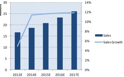
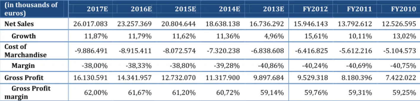
SALES ... 33
9.1.1.1.
LIKE-FOR-LIKE (LFL) GROWTH ... 34
9.1.1.2.
CURRENCY ... 34
9.1.1.3.
STORES EXPANSION GROWTH ... 34
9.1.2.
COSTS ... 35
9.1.2.1.
COST OF GOODS SOLD ... 35
9.1.2.2.
OPERATING EXPENSES ... 36
Equity Valuation of Inditex
2014
9.1.3.
AMORTIZATIONS AND DEPRECIATIONS ... 37
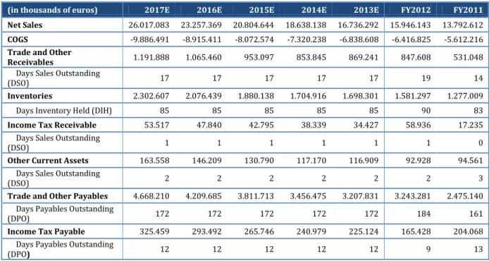
9.1.4.
CHANGES IN WORKING CAPITAL ... 38
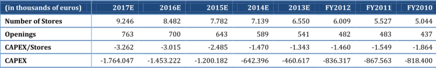
9.1.5.
CAPITAL EXPENDITURES ... 39
9.1.6.
COST OF CAPITAL ... 40
9.1.7.
PERPETUAL GROWTH RATE ... 40
9.1.8.
NUMBER OF SHARES ... 42
9.1.9.
FINANCIAL ANALYSIS ... 42
9.1.9.1.
KEY PERFORMANCE INDICATORS ... 43
9.1.10.
STOCK ANALYSIS ... 44
10.
VALUATION RESULTS ... 45
10.1.
DCF ... 45
11.
SENSITIVITY ANALYSIS ... 48
11.1.
NEW OPENINGS ... 48
11.2.
LIKE-FOR-LIKE (LFL) ... 49
11.3.
COST OF GOODS SOLD (COGS) ... 49
12.
RELATIVE VALUATION ... 49
12.1.
PEER GROUP... 50
12.2.
MULTIPLES VALUATION ... 50
13.
VALUE AT RISK (VAR) ... 51
Equity Valuation of Inditex
2014
15.
CONCLUSION ... 54
16.
ANNEXES ... 56
16.1.
HISTORICAL INCOME STATEMENT, BALANCE SHEET, AND CASH FLOW
STATEMENT ... 56
16.2.
INCOME STATEMENT FORECAST ... 59
16.3.
DCF FORECAST ... 60
16.4.
PEER GROUP – CENTROIDS ALLOCATION ... 61
Equity Valuation of Inditex
2014
1. Introduction
Investors have long searched for a method that would allow them to maximize returns while minimizing risk. While several allocation models have emerged in the literature in the past decades, like Markowitz (1952), the importance of accessing firm value has likewise and even more importantly grown to become one of the most important calculations performed in Finance.
Besides being the basis of all investment transactions when it comes to the investor side –without a proxy for firm value it would not be possible to arrive at a forecast of stock prices – it has become equally important not just as a way of evaluating future cash flows but also in valuating projects, investment decisions, products or divisions. It not only measures a firm’s current performance but it also allows for forecasts of future performance and it is key in cases of Mergers and Acquisitions, for instance, or in the pricing of Initial Public Offerings. One can, thus, say that it presents a financial importance and it is also strategically vital given that it influences the future behavior of companies. Without the knowledge of how much a firm is worth, for instance, it would not be possible for investors to base their financing decisions and allocate their assets into one that maximizes their return. Similarly, when it comes to the firm’s side, evaluating a project is a crucial operation that companies perform every day and allows for future growth and profit.
It is not possible to stress how important equity valuation is today. Even using a wide selection of assets like cash flows, options or dividends or even relying on peer information, it is possible nowadays to access value and compute a firm’s stock price as a way of providing information to all participants of market transactions.
In this thesis, a wide array of valuation methods starting from the Discounted Cash Flow methodology to Multiples valuation will be performed as a way of arriving to a value for Inditex’s stock price. Even though there is not a consensus in the literature to which valuation methods are more effective, by using several valuation methods it was possible to arrive at an accurate prediction for Inditex’s stock price and value.
Additionally, a sensitivity analysis will be performed, where both WACC and growth rate are going to be changed in order to get to different outcomes. Finally, I will compute the Value at Risk to verify the probability of the stock price falling 1%, 5% or 10%.
2. Literature Review
It is not at all times that a company’s market value corresponds to its fair value. Nonetheless, this does not mean that markets are inefficient, particularly since prices will eventually converge to their fair
Equity Valuation of Inditex
2014
value. In order to accurately get a company’s fair value, it is required that a valuation is carried out. There are several valuation methodologies: Discounted Cash Flow (DCF), Multiples valuation, and other approaches such as The Economic Value Added and the Option Pricing Model. Within the DCF model one can still identify a few different approaches: Equity valuation, the Dividend Discounted Model (DDM), Firm valuation, the Adjusted Present Value approach, and the Capital Cash Flow Model, which will be discussed in further sections.
2.1. The Discounted Cash Flow
The DCF methodology is one of the most widely used approaches to evaluate the present value of a company, division, product, or project based on the cash flows it generates. A requirement is that the analysts should be specialists and fully understand the business, the firm’s or cash flows’ risk, as well as the cash flows’ sustainability, argues Damodaran (2002).
The value of the firm according to the DCF method is defined as the present value of its assets discounted at a given discount rate. It is therefore crucial that the analysts verify the company’s essentials and market perceptions in order to better predict the cash flows, however the choice of the discount rate to be applied is also vital. It ought to be thoroughly chosen, given that it is a reflection of the risk of the expected cash flows, as represented in the DCF formula shown in equation 1 below.
Value
(1)
A consideration that arises from this formula is that one should expect to have a higher firm value for companies with more predictable cash flows in opposition to more volatile ones, as stated by Damodaran (2002). Additionally, the author shows that the used intrinsic value is never the real one, since private information causes a distortion in the assumptions based on the public information. The DCF model has a few limitations and as Luerhman (1997) argues, in order to have an accurate valuation, the method should not be applied to companies with neither tax positions or fund-raising strategies nor very complex capital structures.
Damodaran (2002) states that depending on the different types of assets, the also the cash flows will also vary. For instance, if one is taking stocks into consideration, the cash flows would be dividends; if the case is of a bond, the cash flows come from the coupons and the face value; however, if a real project is being analyzed, the cash flows are then the after-tax cash flows. As mentioned earlier, the discount rate will also be a function of the risk of the expected cash flows.
Equity Valuation of Inditex
2014
Model. These methods take into account the cash flows and the discount rate, which differs from one model to another.
2.1.1. Equity Valuation
The Equity Valuation model consists of discounting the cash flows to the equity at the specified cost of equity. In this case, the cash flows to the equity are the residual cash flows after meeting all the expenses, reinvestment needs, tax obligations, interest, and principal payments. Concerning the discount rate - the cost of equity - it refers to the rate of return required by the shareholders of the company. Luerhman (1997) argues that the Equity Valuation model has more complete cash flows, since the DCF cash flows and discount rates are simpler. It is a more specific valuation method when compared to the APV or the valuation of options, since it needs to include the leverage effects in both cash flows and discount rate. In this model the fair value of the firm is given by equation 2, represented below.
Value
(2)
2.1.2. The Dividend Discount Model
The Dividend Discount Model (DDM) is one special version of the Equity Valuation model, where the fair value will be the present value of the expected dividends. Damodaran (2002) states that when investors buy stocks there is an expectation to receive dividends during the time they hold it and a final price for the stock at the end. Therefore, Farrel (1985) argues that this model should be used to define the stock’s attractiveness and also of the stock exchange it belongs to. Moreover, Farrel (1985) states that in this method it is likely to see how the stocks are affected by inflation rate changes and interest rate variations. In the past, the main total returns received by investors were constituted by dividends, according to Foerster and Sapp (2005).
Ang and Liu (2004) argue that the DDM does not take into account any of the stylized effects: time variation in the market risk premium, factor loadings or risk free rates. Through the computation of a variance decomposition of the discount rates, investors should be more concerned with the impact of time-varying interest rates and risk premiums for discounting cash flows. Regarding long horizons, the time variation in risk free rates or betas is more important. The effects of time-varying risk premiums, risk free rates, and betas are of crucial importance for any valuation.
Equity Valuation of Inditex
2014
2.1.3. Firm Valuation
In this situation, and differently from Equity Valuation, Firm Valuation uses the cash flows to the firm instead of to the equity, meaning that the cash flows under consideration are the residual cash flows relating to operating expenses, reinvestment needs, and taxes, but including any payments to either debt or equity holders. In this model the Weighted Average Cost of Capital (WACC) is used as the discount rate in order to account for the advantages and disadvantages of the capital structure, meaning that it includes both costs and benefits from tax shields. A further discussion on the Weighted Average Cost of Capital is presented in section 2.6.5. The value of the firm comes, as a result, through the following formula:
Value
(3)
2.2. The Adjusted Present Value method
The APV model does not seem to arrive at a consensus when it comes to the authors in the literature. Luerhman (1997) starts by arguing that the DCF model is no longer the most accurate methodology to evaluate companies and that business schools and books still teach it because it is standard. He defends that the APV model is now the best, most reliable and versatile model of firm valuation. The APV model splits the company into different parts, evaluates them and then sums up the parts again. Accordingly, and as mentioned by Damodaran (2002), the first step is to assume that the company is only equity financed and, thus the equity is evaluated first and separately. The next step in the evaluation is to add the profits or losses given by the debt part of the company. Finally, the bankruptcy costs have to be taken into consideration. Damodaran (2002) argues that, with this separation, the APV clearly highlights the benefits and costs of debt given that on the one hand the increase in debt generates tax shields and on the other hand it increases the bankruptcy costs. Therefore, the value of the enterprise according to the APV model arrives from the following formula:
Value = Value of all-equity financed firm + PV tax benefits + Expected bankruptcy costs (4)
There is one clear advantage in using the APV model: APV works for most valuations, even in cases where WACC does not. This is due to the fact that it requires less restrictive assumptions. Also, the APV model provides investors with much more information than the DCF model since the APV is not just giving the final fair value but also the different parts where the value stays. On the other hand, Luerhman (1997) argues that the DCF model is a lot easier to use than APV since it uses only one discounting operation. Moreover, there is another disadvantage stated by Damodaran (2002) which is
Equity Valuation of Inditex
2014
the fact that investors tend to ignore the probabilities of default and bankruptcy costs because they are considerably hard to estimate.
2.3. The Capital Cash Flow Model
Goedhart, Koller, and Wessels (2005) state that the Capital Cash Flow model is very similar to the models discussed before but with the particularity that the interest tax shields are summed up to the free cash flow and these are discounted at the unlevered cost of equity. As a result, the enterprise value is given through formula 5.
Value = PV (Capital Cash Flows) =
(5) Since future cash flows are predictable, all the models mentioned earlier are reliable and considerably simple to use. Problems appear when this does not happen which is the case of firms in trouble, cyclical firms, firms with unutilized assets, firms with patents or product options, firms in the process of restructuring, firms involved in acquisitions and private firms, for instance.
2.4. Multiples Valuation
As stated beforehand, there are several methods for valuing projects, divisions, and companies, although senior executives and managers see the DCF model as the most accurate and flexible one. However, the DCF model takes into consideration several variables such as the company’s Return On Investment Capital (ROIC), the growth rate, and the Weighted Average Cost of Capital (WACC), which might make the computations somewhat difficult if they are not available. Another drawback with this method, other than the fact that it should only be used to evaluate more complex business structures, is that it relies on several assumptions and whenever the case of mistakes in these assumptions arise, is can lead to incorrect valuations. Nonetheless, in order to make the forecasts more useful, some authors believe that a company’s multiples should be compared to the multiples of other corporations. This kind of analysis allows helping the company to check its cash flow forecasts, its own performance against that of its competitors’ or even to compare its strategy to the main drivers of its industry. Goedhart, Koller and Wessels (2005) argue that the reliability of the valuation can be improved by choosing companies within the same industry. Fernandez (2002), on the other hand, states that multiples valuation is very useful but should not be carried out on its own and instead be supported by other valuation methods.
The setback of using the multiples method has been the fact that they have been historically misunderstood and misapplied. Goedhart, Koller, and Wessels (2005) mention that one of the problems presented with the multiples valuation resides in the fact that most analysts do not accurately apply it
Equity Valuation of Inditex
2014
and fail applying factors like the growth rate, Weighted Average Cost of Capital (WACC) or Return On Invested Capital (ROIC). Managers often use the industry average, although the fact is this usually not the best to make use of since even within the same industry companies may have very different expected growth rates, Returns On Investment Capital and capital structures. Therefore, a peer group should not be selected by relying on the industry as a whole. In order to get an accurate peer group, indicators such as capital structure, growth rate, cost of capital and profitability must be taken into consideration. There are several lines of thought in the literature in what concerns the formation of peer groups. Foushee et al. (2012) states that the peer group should be constituted of companies from the same market and subject to the same macroeconomic events. Damodaran (2002), for instance, does not agree and argues that the peer group should be based on similar potential growth, risk, and cash flows.
There are three setbacks when evaluating a company with multiples. Firstly, expectations regarding the ability of each company to create value are different and thus only companies with similar ROIC and growth rates should be chosen, as Goedhart, Koller, and Wessels (2005) state. Secondly and likewise stated by the same authors, the use of multiples can lead to different conclusions. Lastly, depending on the contexts, multiples can either be very useful or meaningless.
In order to make accurate use of multiples, Goedhart, Koller, and Wessels (2005), argue that there are four basic principles that every company should take into consideration: the use of peers with similar ROIC and growth projections, forward looking multiples, enterprise multiples, and the adjustment of enterprise value multiples for non-operating items. Liu, Nissim, and Thomas (2002) share the same opinion and argue that the multiples valuation should be based on the forward earnings in order to get a more precise explanation of stock prices.
Finding peers with similar ROIC and growth projections is not an easy task. Occasionally, companies list their main competitors in their annual reports. The majority are found by looking at the company’s specific industry but this is often a wide number of different companies with extremely different multiples. These differences amongst the companies’ multiples arise due to the fact that some enterprises have economies of scale, products of higher quality than its competitors, better access to the customers or to financing. Other than that, the products that companies sell, how the companies generate revenues and profits, and their growth rates also reflect different multiples. At last, and after taking all these parameters into consideration, the peer group should be smaller and consequently more accurate to give a better perspective of the industry that the company finds itself.
Empirical evidence tells us that the computation of the multiples should be based on forecasts rather than historical data given that they are more precise. But whenever there are no reliable forecasts
Equity Valuation of Inditex
2014
available the latest available historical data should be used. Also, the one-time events should be eliminated.
The use of the enterprise value multiple to EBITDA is one of the alternatives to the widely used Price-Earnings ratio. Firstly, because the P/E ratio is affected by the capital structures and, on the contrary, the EV/EBITDA multiple is less vulnerable to changes in the capital structure. Secondly, and since P/E ratio is based on earnings, it can be affected by one-time events.
On the other hand, as the EV/EBITDA hides non-operating items, it should be adjusted by:
Excess cash and other non-operating assets - As the enterprise value should not contain excess cash, the non-operating assets have to be separately evaluated;
Operating leases - In order to have an accurate EV/EBITDA multiple, the value of the leased assets should be added to the debt and equity in market values. Also, the implied interest expense should be added to the EBITDA since these sums are not of the same magnitude;
Employee stock options - In order to have the most precise EV/EBITDA multiple, one should add the present value of all employee grants currently outstanding and next subtract the new employee option grants;
Pensions - In order to have the real value of the enterprise, the value of pension liabilities should be added to it.
There are also other multiples besides the ones mentioned before that are used exclusively for specific situations. For instance, to evaluate different companies, the Price-to-Sales multiple should be appropriate. The same happens with the enterprise value-to-EBITA multiple, where besides the assumption of similar companies having similar returns on incremental investments and growth rates, it is assumed that companies have similar operating margins. Additionally, Goedhart, Koller, and Wessels (2005) state that ratios built on enterprise values are more accurate since they are less vulnerable to capital structure changes. Another point of view is mentioned by Liu, Nissim, and Thomas (2002), where they state that EBIT and sales do not have as interesting performances as the adjusted EBITDA.
As mentioned before, another widely used multiple is the Price-to-Earnings (PER), which is easier to use in cases of valuations of companies in different cycles. This means that it is more flexible than other multiples given that they allow for the expected growth rate to vary in different companies.
Beaver and Morse (1978) state that the Price-to-Earnings (PER) multiples identify momentary aspects of the actual earnings and can predict the future ones. Goedhart, Koller, and Wessels (2005) disagree and say that the PER ratio is usually misapplied because non-operating and non-recurring items are
Equity Valuation of Inditex
2014
fixed in the earnings figures. Regarding new companies’ valuation that normally have losses and relatively low sales, a good tool would be non-financial multiples that compare the company’s value to non-operating statistics, such as the number of a website’s visitors or the number of subscribers. Nonetheless, if it is not possible to convert the subscribers or the visitors into either cash flows or profits, the nonfinancial multiples are is useful at all and therefore a multiple built on financial forecasts would provide better and more reliable results.
2.5. Other approaches
2.5.1. The Economic Value Added
The economic value added is the real value created by an investment and is computed through the following formulas represented below.
Economic value added = (Return On Capital Invested –Cost of capital) x Capital invested (6) Economic value added = After tax operating income – (Cost of capital x Capital invested) (7)
The purpose of this method is to highlight the owners interest since the cost of capital is their reward for the investment made in the company. Timo and Virtanen (2001) say that in normal circumstances the economic value added is indifferent to its cost of debt factor but not to its cost of equity component. Economic value added has been one extension of the net present value method and therefore a company or project can be evaluated through equation 8.
NPV
(8)
2.5.2. The Option Pricing Model
There are some particular situations in which the DCF model does not work properly, such as options. Some analysts use the DCF with special clauses to evaluate opportunities. Frequently, this results in strategic options being undervalued since the DCF model is discounted at lower rates than regular investments, as Luerhman (1997) argues. In other cases, analysts have started to use the Option Pricing Model instead of the DCF. An option is a right that can be exercised or not, at the option of the option holder (purchaser), linked to an underlying asset with a strike price, allowed to be exercised until the expiration date. The option’s payoff comes through the difference between the asset value and the exercise price.
Equity Valuation of Inditex
2014
The current value of the underlying asset - Since the option value varies with the value of the underlying asset;
The variance in value of the underlying asset, which means the higher the variance in the underlying asset, the higher value of the option because it has the potential of gaining more value with large price movements for both calls and puts;
The dividends paid on the underlying asset because each time dividends of an underlying asset of the call option are paid, the value of the option decreases;
The strike price of the underlying asset, since the higher the strike price of a call option, the lower value of the option;
The time to expiration of the option, for both calls and puts. The longer the time of an option the greater the value because there is a bigger range of time to exercise the option;
Finally, the riskless interest rate corresponding to the life of the option. Besides being a cost of opportunity, the higher the interest rate, the greater value of a call option because it is a cost that does not have to be paid.
The most used models to evaluate options are the Binomial and the Black & Scholes models, which find the option’s value through a portfolio’s replication, based on the underlying asset and the risk free rate. As Damodaran (2002) states, these models are also used to evaluate other assets besides options but with similar features that could not be evaluated in traditional methods. Luerhman (1997) argues that even though pricing models are very useful they should not be used as the only valuation method but instead as a supplement to other methods such as the Black & Scholes. Even though Luerhman (1997) states that this is his favorite method, he also presents some disadvantages to it as the difficult application to corporate problems and the fact of being necessary more time to learn it which makes it as a result, a more expensive method.
2.6. Other considerations
2.6.1. Present Value of tax shields
One of the advantages of using debt is the appropriation of tax shields. In order to get the present value of tax shields and obtain the real effect of the financial side effects, and as mentioned earlier, it is crucial that the discount rate computed is an accurate reflection of this. Amongst the authors, however, there is no consensus concerning the use of the discount rate. While some say that it should be just an interest rate associated with the tax shields, Modigliani and Miller (1985, 1963) argue that the risk-free rate should be the discount rate to use in tax shields. Among Damodaran (2002), Goedhart, Koller, and Wessels (2005) and Luerhman (1997) there is a consensus where all of them state that the cost of debt should be the discount rate used since it comes directly from debt and it should be exposed to the same
Equity Valuation of Inditex
2014
risk level, thus providing to be a reliable proxy. Fernández (2004), on the other hand, points out the need to distinguish between the value of tax shields and its present value, and argues that the value of tax shields refers to the difference between the present value of taxes of the unlevered and levered companies.
2.6.2. Terminal Value
In a company’s valuation it is known that often the company cannot maintain its growth rate in convenient levels forever. As it grows, it becomes harder to keep high growth rates. Also, most companies do not last forever and there will be the need to liquidate the company at some point in time. In order to introduce the liquidation value in the firm valuation, the terminal value of the company has to be computed. Since the cash flows are infinite, they should be calculated for the years that the company will last and, afterwards, this should be summed to the terminal value. Therefore, the company’s value is calculated through equation 9.
Firm Value
+
(9)
Analysts should give more importance to the breakdown of this variable rather than spending excessive amount of time on the next years’ forecasts, as state by Young et al. (1999). Also, Goedhart, Koller, and Wessels (2005) state that the terminal value should be calculated at the end of the explicit period. In order to get an accurate valuation the explicit period should be large enough and therefore between five and seven years ought to be an appropriate time frame to use.
2.6.2.1. Computation methods
There are three approaches to estimate the terminal value: the liquidation value, the multiple approach and the stable growth model.
2.6.2.1.1. The Liquidation value
The liquidation value can be estimated in two different ways. The first is based on the current value of the company’s assets, taking into account the inflation rate, through formula 10.
Expected liquidation value = book value of the assets (1 + Inflation rate) average life of the assets (10)
The only disadvantage of this approach is that it is based on the accounting book value and therefore does not reflect the real earning power of the assets.
Equity Valuation of Inditex
2014
Regarding the second way of computing the liquidation value, it is related to estimating the earning power of the assets. Thus, one should be careful to use an accurate discount rate to discount the expected cash flows.
2.6.2.1.2. The multiple approach
According to the second approach - using multiples - the terminal value arises from the application of a multiple to the expected company’s revenues in the liquidation year. Although this method is much simpler and easier to use, it requires caution. At the end, if this is the method that is chosen, it must be taken into account that the estimation comes from using comparable firms and thus the terminal value will result in a mix of both discounted cash flows and relative valuations.
2.6.2.1.3. The growth stable model
Finally, the growth stable model relies on the basic concept that the company will be liquidated at the end of its life. There are a few ways to compute the terminal value through this approach, depending on the assumptions that are made. If, for instance, the assumption is that the cash flows will grow at a constant rate until the end of the firm’s life, then formula 11 ought to be used:
Terminal value =
(11)
Depending also if the valuation is being made about equity or the firm itself, different formulas need to be used:
Terminal value of equityn =
(12)
Terminal valuen =
(13)
2.6.3. Risk Free Rate and the Risk Premium
In all valuation models, a required rate of return by investors is present as a necessary input to make an investment in a project or in a company. This, on the other hand, is dependent on the risk premium, which consists of the difference between the risk free rate and the market rate of return.
The first step to take is to define what a risk free asset is. In order for an asset to be considered as risk free, its expected returns must be certain, which means that the expected returns must be equal to the actual returns. Secondly, risk of default cannot be present, meaning that it cannot be a security issued by private firms because even the most certain, safest and largest companies have at least some risk of default. In order to accomplish this parameter, only securities issued by the government can be
Equity Valuation of Inditex
2014
accepted, not because they are the safest companies but because they control the printing of currency. Finally, reinvestment risk cannot be present as well. For instance, in a year investment, a three-month Treasury bill rate, even with no default risk is not a risk free rate since there is no certainty of what will be the rate in the next three months. Even if we take into consideration a three-year Treasury bond, it is still not a risk free investment because it is not possible to predict today at what rate the coupons will be reinvested in the future. Therefore, only a three-year zero coupon can be considered since it is the only one that ensures totally certainty about the expected returns.
The basic idea behind the equity risk premium is that the riskier the investment the higher the expected return. In line with that, a safer investment should return a smaller gain. Therefore, and according to Damodaran (2002), the expected return of an investment should be the sum of the risk free rate plus an extra return to compensate for the risky investment.
It is still important to mention that the equity premium, according to Damodaran (2012), has distinct ways of being measured, which may lead to different results: while the first relies on historical data, the second - the ex-ante equity premium - is a forward-looking measure. Damodaran (2012) also mentions the Survey Approach, in which investors or managers are questioned so as to find out their own expectations with respect to future equity returns. Nevertheless, among the authors there does not seem to be an agreement on how to measure the risk and the appropriate interest rate to compensate for it. Risk should be broken into two different parts: the term-specific factor that is related to the risk of the investment itself and the market risk factor that takes into consideration the risk that affects all investments. The term-specific risk is diversifiable and the more investments a portfolio has, the less the term-specific risk and a certain point can even be achieved where it is totally removed. However, the market risk is not diversifiable and this will always be the same independently of the investments made. This is the risk that should be rewarded.
Total risk can be minimized as long as the diversifiable risk can be equally minimized as well. Nevertheless, the non-diversifiable risk will be always be the same regardless of the number of stocks. There are four models that measure the risk and return of an investment: Capital Asset Pricing Model (CAPM), Arbitrage Pricing Model (APM), Multifactor Model and Proxy Model. They all come to an agreement when discussing the split-up of these two types of risk but not in how to measure the non-diversifiable (market) risk. In models that can measure the market risk with beta, the expected return arises from the following formula:
Equity Valuation of Inditex
2014
In the first model – the CAPM – and since there is no private information neither transaction costs, beta is measured against the market portfolio. There are three different approaches to estimate discount rates through the CAPM: by using firm-level, industry-level, and market-level as measures of risk. Regarding the APM, and assuming there is no arbitrage, investments which have the same exposure to market risk must have the same trading price. Concerning this, betas must be measured in terms of the unspecified multiples of the market risk components.
Concerning the Multifactor model, the assumption is the same as the APM model and therefore betas have to be measured against multiple specified macroeconomic factors.
Finally, with respect to the Proxy model, there is the assumption of longer periods and higher returns on investments that must compensate for higher market risk.
2.6.4. Cost of Capital
In order to finance their projects, companies need to raise money from investors, which can be either equity or debt holders. Still, they require a rate of return, the cost of capital. Luerhman (1997) says that both costs of debt and equity should be seen as opportunity costs since they reflect their own time value and risk premium.
The cost of equity is the return rate that equity investors require to invest in a given project of the company. This cost is composed by the risk free rate and a risk premium, which considers also the market risk, and takes into consideration the beta of the company, as it was stated before. Therefore, Damodaran (2002) and Koller et al (2005) agree when it comes to the definition of the cost of equity represented in equation 15.
Ke = Rf + (E(Rm) – Rf) (15)
There are three ways to estimate the betas of a company: the first is to use historical market betas while the second possible approach is to use fundamental betas, and finally, accounting betas.
Concerning the cost of debt, this refers to a cost that measures the capacity of a firm to repay its debt. It includes the risk free rate plus the default risk of the firm (and linked to default spread). The higher the default risk of the firm, the higher cost of debt. The cost of debt also includes the tax advantage that arises from debt, taking into consideration that the interest is tax deductible and there are some benefits on it, as it was previously mentioned. The after tax cost of debt comes through formula 16 represented below.
Equity Valuation of Inditex
2014
Damodaran (2002) states that the default risk and spread are based on two different parameters. First, the recent borrowing history of the company, where from other loans that companies have with banks and other financial institutions, it is possible to check what the precious default spreads charged were. Secondly, to estimate a synthetic rating which means to assign a rating to the company based on its financial ratios, taking also into account the rating classes already assigned by others.
Occasionally, companies have difficulty when it comes choosing the correct tax rate. In this case, the one that should be used is the marginal tax rate since it is the one at which the last dollar of income is taxed, as states Goedhart, Koller, and Wessels (2005).
2.6.5. Weighted Average Cost of Capital
The Weighted Average Cost of Capital plays a crucial part when evaluating a firm’s free cash flow to the firm, after getting estimates of the firm’s future free cash flows.
Given that it simultaneously reflects the risk of the cash flows, the time value of money (the risk-free rate) and the risk premium that investors demand as a compensation for the risk they undertake, it is widely accepted in the literature as an adequate and accurate proxy for risk.
The main concept behind WACC is that it weights proportionally each category of capital against its capital structure, being thus a weighted average of all the sources of the firm’s financing like common stock, preferred stock, bonds, and any other long term debt instrument that the company may use. In addition, the after-tax WACC is also a broad measure for risk since it already captures the benefits for firms that hold debt, through its tax shields.1 One must not forget, however, that some factors like
issuing costs, subsidies hedges, exotic debt or dynamic capital are specific financing programs for which the WACC needs to be adjusted, states Luerhman (1997).
There are still two important assumptions that ought to be made by managers before considering using WACC as a way of valuating projects, since every variable that goes into the formula is referent to the whole company:
1. By accepting the project, the firm is taking a compromise on how the project should not lead to a change in the firm’s debt ratio, meaning that the firm needs to commit to keeping the debt ratio constant over time (which would mean a need of adjusting the borrowing accordingly with the value rising over time);
2. The project needs to be as risky as the average of the firm’s other assets and if the project has a different risk then the WACC is no longer a suitable measure to be used. If firms use
Equity Valuation of Inditex
2014
WACC to discount every type of projects, disregarding how risky they are with comparison to the company itself, the firm will accept too many high-risk projects and reject too many low-risk projects. In fact, “it is the project risk that counts: the true cost of capital depends on the use to which the capital is put."2
One last important thing to mention is the case of conglomerate companies that operate into different business segments or different industries, with different characteristics and different risk. Even though this is not the case of Inditex, it is worth pointing out that the ideal would be not to use a single WACC for the entire company but let each division discount its own projects with its own WACC.
Taking all these factors into account, the WACC is given through equation 17, where D/V is the target debt level of the company, measured in market values and E/V is the target for equity level, also in market values. Thus, Kd is the cost of debt, Ke the cost of equity, and Tm the company’s marginal tax rate.
WACC = Kd (1 – Tm) + Ke (17)
Therefore, the cost of equity is computed through the CAPM using the risk free rate, market risk premium, and the company beta, as the calculation inputs. The after tax cost of debt takes into consideration the risk free rate, default spread, and the marginal tax rate. Finally, the capital structure is just the proportion of the debt and equity in the company. Fernandez (2013) argues that while the cost of debt should be seen as a cost, the cost of equity – required rate of return – can be seen either as a cost or a return.
The WACC has, however, some limitations. The first one is presented by Luerhman (1997) and he defends that analysts often misapply it when ignoring some financial side effects like the cost of financial distress that comes along with the corporate leverage. Luerhman (1997) and Fernandez (2004) share the same opinion concerning the debate on how analysts use book values for the weights when they should be using market values instead.
2.7. Conclusion
After carefully weighting all the advantages and disadvantages of each method, I believe the DCF model should accurately evaluate a company’s fair value. The DCF methodology is very flexible and is focused on the cash generation, meaning that it is based on the assets’ fundamentals and not on market feelings or observations and shows the underlying characteristics of the company, which makes it easier for a buyer to understand the firm’s business. Although the multiples valuation opens the scope of the
Equity Valuation of Inditex
2014
valuation so as to take into consideration the industry or a representation of it through the peer group, I believe it is needed a good method to be used but as a supplement method to the DCF, and not as the main valuation tool.
3. History
The largest Spanish retailer and certainly one of the most important companies in the retailing and apparel industry is Industria del Diseño Textil, SA, mostly known as Inditex. Currently, its CEO is Pablo Isla, which was appointed by Amancio Ortega, Inditex’s founder and previous CEO, and he is currently the major shareholder. Amancio underlined Pablo’s youth and experience as a value added for the Group.
Amancio Ortega began his career very early at the age of 13 in the clothing industry He started off as a messenger boy for a shirt maker named Gala, and eventually became a store manager years later. In 1972 he founded his first clothing manufacturing company, Confecciones Goa, in Coruña, selling not only for Spain but also for a few more countries in Europe. With already some experience, Amancio opened his first store in Coruña called Zara, in 1975. It was particularly popular because on the one hand he built a very successful and unique business model based on the combination of fashion and high quality products at low prices and on the other hand the stores were placed in strategic downtown locations. Given the great success verified, a validation of this business model, a considerable number of stores along some major Spanish cities opened in the next few years.
In 1985 he created Inditex as the holding company. Later, in December 1988, Inditex launched Zara’s first overseas store in Oporto, Portugal, followed by openings in New York in 1989, and in Paris in 1990. During the 1990s, Inditex suffered a vast expansion, launching stores in 29 countries in three different continents: Europe, America and Asia. The Group acquired and created new companies such as Pull and Bear, Massimo Dutti, Bershka and Stardivarius, in order to reach different segments and formats for different types of customers. During the 2000’s, Inditex launched three new brands, Oysho (2001), Zara Home (2003), and Uterqüe (2008). These three new brands delivered quite different products from the others given that Oysho sells lingerie, Zara Home with a totally different concept focuses on decorating and furniture and, finally, Uterqüe sells quotidian products, such as jewelry, hand bags and sun glasses. In 2001, Inditex went public through an IPO. Amancio Ortega sold 26% of his shares, which made the company to be valued at almost €9 billion. Therefore, Amancio and his family retained 70%, with the remaining 4% belonging to management and employees. Two months later, in July 2001, the share price was 25% higher than the initial price, with Inditex’s value surpassing the € 11 billion mark.
Equity Valuation of Inditex
2014
4. Inditex today
Currently, Inditex is present in 86 different countries with 6249 stores. Inditex owns 8 different brands: Zara, Pull and Bear, Massimo Dutti, Bershka, Stardivarius, Oysho, Zara Home, and Uterqüe. According to the financial data in the last annual report (2012), Zara is by far its main brand with 29% of its stores (1808 of 6249)3, and representing 66.11% of total sales (10.541 € million out of 15.946 € million)4.
These different brands allow the Group to diversify its target customers and therefore reach different market segments.
Figure 1 – Percentage of store contribution for Total Sales
Source: Inditex’s annual reports
Figure 2 – Number of worldwide stores at October 2013
Source: Inditex’s annual reports
According to Inditex’s annual 2012 report, the Group sales are divided into four main areas: Spain, Europe Ex-Spain, Americas, and Asia (Rest of the World). As one can see in Figure 3, Europe Ex-Spain represents its major selling area with 47.9%, followed by Spain with 22.2%, Asia with 16.3%, and finally, Americas with 13.6%. As part of its internationalization strategy, Inditex has made an 3 Last update in 31/10/2013 4 Annual report of 2012 66.11% 6.81% 7.11% 9.31% 6.03% 1.97% 2.20% 0.46% Zara Pull and Bear Massimo Dutti Bershka Stradivarius Oysho Zara Home Uterqüe 1808 164 834 649 934 842 542 388 88 Zara Zara kids Pull and Bear Massimo Dutti Bershka Stradivarius Oysho Zara Home Uterqüe
Equity Valuation of Inditex
2014
investment in Asia and it expects to grow even more in this part of the world, so as to benefit from the large number of customers.
Figure 3 – Percentage of Sales by World Region
Source: Inditex’s annual reports
Concerning ownership’s stores and taking into account the data available in their last annual report, Inditex owns 87.3% of the stores, with the remaining 12.7% being franchised stores.
Figure 4 – Number of Stores owned by Inditex
Source: Inditex’s annual reports Figure 5 – Number of Franchised Stores
Source: Inditex’s annual reports 22% 48% 14% 16% Spain Europe Ex-Spain Americas Asia 30% 3% 13% 10% 15% 12% 9% 6% 2% Zara Zara Kids Pull and Bear Massimo Dutti Bershka Stradivarius Oyshio Zara Home Uterqüe 25% 0% 15% 11% 16% 19% 7% 5% 2% Zara Zara Kids Pull and Bear Massimo Dutti Bershka Stradivarius Oyshio Zara Home Uterqüe
Equity Valuation of Inditex
2014
5. Business model
Inditex states that its success is due to its flexible business model: Stores, Design, Manufacturing and Distributing. This model allows the company to adapt to every situation. Besides the fact that its main competitors have chosen the outsourcing model, Inditex opted for the vertically integrated model. This means that the Group fully controls the entire supply chain, starting with Design, going through both Manufacturing and Distribution, and finishing in the Stores.
The first step of the supply chain is the Design. This is a crucial step since, as previously mentioned, the Group has different brands with different types of customers of different ages and has thus to adapt. There is thus a vast team of more than 1000 professionals responsible for the different products. Taking into account all the information collected in the stores and online data, this team creates more than 30000 products as fast as possible, being the key to have high fashion products, combining the latest trends with low costs.
Concerning Manufacturing, nearly half of its production is made by local suppliers among Europe which facilitates the entire process. Inditex has its own Code of Conduct for Manufacturers, which allows to building close and ethical relationships of trust and stability. The other half of the production occurs in owned factories. The majority of these factories are in Spain which again makes the process easier. In both cases, the relationships are tight and therefore make the vertical integration possible. Only this way can the throughput time be reduced to 2 weeks, against an average of 6 weeks in the whole industry.
Distribution is the process that ensures that the products are delivered in the stores within the deadline. Before going to the stores, products pass through a distribution center in Spain (mainly located in Madrid, Barcelona, Coruña). The distribution process is conducted twice a week and always contains new products. This way, Inditex can guarantee that the products are delivered to Europe in within 24 to 36 hours, and to the rest of the world within no more than 48 hours.
Finally, the last step of this successful business model is the Stores. Inditex does not spend any money in advertising. Instead, they would rather invest in stores locations, with a large number of people in circulation and with a tremendous architectural design as well as huge well-designed shop windows. Another concern is the top-class customer care notion that every Inditex’s employee has. The online stores are still growing and are also becoming gradually more important.
Equity Valuation of Inditex
2014
6. Financial Analysis
In order to perform a precise and exact valuation of Inditex, it is necessary to carefully analyze historical information as a way of further understanding the values and the way of the company operates. For that, I will take into consideration the last seven years, which I believe to be a period large enough to allow one to make an accurate forecast and to understand how the company operates. Figure 6 – Inditex’s Income Statement
(in thousands of euros) FY2012 FY2011 FY2010 FY2009 FY2008 FY2007 FY2006
Net Sales 15.946.143 13.792.612 12.526.595 11.083.514 10.406.960 9.434.670 8.196.265 Cost of Merchandise -6.416.825 -5.612.216 -5.104.573 -4.755.505 -4.492.720 -4.085.959 -3.589.276 Gross Profit 9.529.318 8.180.396 7.422.022 6.328.009 5.914.240 5.348.711 4.606.989 Gross Margin 59,76% 59,31% 59,25% 57,09% 56,83% 56,69% 56,21% Operating expenses -5.604.783 -4.919.328 -4.452.211 -3.952.702 -3.707.887 -3.226.369 -2.800.243
Other expenses and income, net -11.578 -3.396 -3.604 -1.118 -19.497 26.501 -17.060
Gross operating profit (EBITDA) 3.912.957 3.257.672 2.966.207 2.374.189 2.186.856 2.148.843 1.789.686 EBITDA Margin 24,5% 23,6% 23,7% 21,4% 21,0% 22,8% 21,8% Amortization and depreciation -796.117 -735.666 -675.738 -645.801 -578.320 -496.663 -433.427
Net operating profit (EBIT) 3.116.840 2.522.006 2.290.469 1.728.388 1.608.536 1.652.180 1.356.259 EBIT Margin 19,55% 18,29% 18,28% 15,59% 15,46% 17,51% 16,55% Financial results 14.129 37.006 31.116 3.782 -21.599 964 -14.035
Equity accounting losses 0 0 0 0 0 -7508 -2786
Profit before taxes (EBT) 3.130.969 2.559.012 2.321.585 1.732.170 1.586.937 1.645.636 1.339.438 Income tax -763.956 -613.480 -580.305 -410.033 -325.322 -387.872 -329.502
Net profit 2.367.013 1.945.532 1.741.280 1.322.137 1.261.615 1.257.764 1.009.936
Source: Inditex’s annual reports
In the income statement, represented in Figure 6 above, and starting by the Gross Margin and the EBITDA Margin, it is possible to verify that the company has been consistently profitable over the past few years. For instance, the Gross Margin has been stable varying from 56% to 59%. According to the EBITDA Margin it is possible to see that it has also been stable during the last years, from 21% to 24%, which is considerably better than the industry, as accounted by Damodaran5 (14% - Apparel).
Even in troubled years such as 2008 and 2009, Inditex was able to keep its margins and to keep its sales growing at a normal pace. It was possible to support the sales growth with the investment made in international expansion from previous years.
Another measure of profitability is the Return On Equity (ROE6), which is the ability of the company to
return the money to the shareholders and it is shown in Figure 7.
Equity Valuation of Inditex
2014
Figure 7 – Inditex’s historical Return on Equity
2012 2011 2010 2009 2008 2007 2006 2005
ROE 27,91% 26,09% 27,11% 24,62% 26,57% 29,83% 29,10% 27,76% Source: Inditex’s annual reports and own analysis
It is possible to verify that the ROE has been consistent between 27% and 29%. The values presented prove to be higher than the average of the industry as computed by Damodaran7 (17% - Apparel). Apart
from the fact that Inditex has been very profitable for the past years, ROE takes into consideration the capital structure, with the company presenting almost no debt in the past few years.
Figure 8 – Inditex’s historical Capital Structure
Capital Structure 2012 2011 2010 2009 2008 2007 2006 2005
Debt ratio 0,05% 0,02% 0,06% 0,09% 0,28% 0,99% 1,34% 2,54%
Equity ratio 99,95% 99,98% 99,94% 99,91% 99,72% 99,01% 98,66% 97,46% Source: Inditex’s annual reports and own analysis
The debt ratio has been almost zero only due to the fact that the company has been generating great cash flows and still has enough to reinvest money back into the company. In the case of reinvestment, this concerns the opening of new stores, with the company clearly relying on this expansion strategy as a way of being financially healthy.
7. Industry Analysis
The retail industry is still growing worldwide despite the difficult times and crisis that is being experienced. What is expected for the next years in this industry is that retail companies with headquarters in Europe will increase their dependence on foreign markets. While Europe is still experiencing a crisis, and it will take time to fully recover from it, countries in emerging markets like Asia and Africa are growing at a very fast pace.
This industry is changing as fast as technology. The combination of both physical and virtual world is changing the way customers think. The basis of this rapid change is mobile devices, digital media and tablets which are already equipped with shopping applications. The main goal nowadays for the traditional retailers is to integrate these two worlds. The retail industry has become a technological industry for two main reasons: Firstly, it is easier to control and monitor the entire process, from the production, to the customers, for instance. Secondly, online stores must also be taken into consideration, given that they play a vital role in today’s markets. Online sales are not replacements for the traditional ones but, instead, complementary. Actually, the two main points of online sales are that online sales reach new customers and existing customers buy more through online platforms.
7 http://pages.stern.nyu.edu/~adamodar/
Equity Valuation of Inditex
2014
Two great cost savings for online stores can be highlighted: the cost associated with the store renting and staff costs.
In terms of population of digital buyers, countries like China, the US, Japan, the UK, Germany, France, and Russia are those with the highest number of potential customers. The population in these countries has high potential density, which represents thus a huge potential opportunity for online sales.
8. Macroeconomic Analysis
Currently, the main factor that influences the retail and apparel industry is the cotton price. I believe the cotton price will be the major discussion in the margins of years to come, since tissue and materials represent around 60% of the Costs of Goods Sold. From March 2011 until September 2012, and since then, the cotton prices have, however, stabilized.
Regarding cotton production, it is expected to be 146 million bales in 2020 (30 million bales more than in 2011)8. Equally important is the production and consumption of cotton in Europe, given that the
higher percentage of Inditex’s market share is in this part of the world. However, it is expected to decrease until 2020, which will result in major companies like Inditex to invest in markets much more attractive such as China who is projected to use about 41% of the world cotton mill in 2020. The retail industry in China will still be growing but at a slower pace for the next 10 years, due to the increase in labor costs. As a result of this, some of the mill capacity will be moved to other Asian countries such as Vietnam, Bangladesh, and India9. In addition to that, real GDP is expected to grow by 2% to 3% in
developed countries and by around 5% to 6% in developing countries until 202010.
Finally, and according to the feeling in Southern European countries, which are in financial distress, sales in these areas will not grow or at least not at the same pace as other markets like the rest of Europe or Asia. This is mainly verified for companies like Inditex, which has its headquarters in Spain, and a major part of its sales are in countries like Spain, Portugal, Greece, and Italy.
9. Valuation
In this section I will use the Discounted Cash Flow (DCF) method as the main valuation tool to compute Inditex’s share price and it will be done on a consolidated basis. In order to compute the firm’s Free Cash Flows to the Firm (FCFF), I used historical data, mostly since 2003, and with a five year explicit period.
8 According to “Global Cotton Baseline 2010/11 – 2020/21” from Cotton Economics Research Institute, March 2011 9 According to “Global Cotton Baseline 2010/11 – 2020/21” from Cotton Economics Research Institute, March 2011