Land suitability analysis to assess the potential of public open spaces for urban agriculture activities

(1)

Land Suitability Analysis to Assess the

Potential of Public Open Spaces for

Urban Agriculture Activities

Dissertation submitted in partial fulfillment of the requirements for the Degree of Master of Science in Geospatial Technologies

February 24, 2020

_______________________________________

Maicol Fernando Camargo Hernández

mfcamargoh@gmail.com https://github.com/mfcamargoh

Supervised by:

Hanna Meyer

Institute for Geoinformatics University of Münster

Co-supervised by:

Judith Verstegen Institute for Geoinformatics

University of Münster

and

Pedro Cabral

Information Management School Universidade Nova de Lisboa

(2)

ii

Declaration of Academic Integrity

I hereby confirm that this thesis on Land Suitability Analysis to Assess the Potential of Public Open Spaces for Urban Agriculture Activities is solely my own work and that I have used no sources or aids other than the ones stated. All passages in my thesis for which other sources, including electronic media, have been used, be it direct quotes or content references, have been acknowledged as such and the sources cited.

February 24, 2020

___________________________________

I agree to have my thesis checked in order to rule out potential similarities with other works and to have my thesis stored in a database for this purpose.

February 24, 2020

(3)

iii

Acknowledgments

The idea about this research came to my mind when I was visiting the urban orchard of my aunt Elena Villamil located in downtown Bogota. I was fascinated by the idea of harvesting our food and the social, environmental and cultural benefits involved in urban agriculture practices. Since that moment, I wanted to develop my thesis related to urban agriculture to benefit the population of my city. For this and much more, infinite thanks to my aunt for inspired me with her passion for this humble and rewarding activity. From my heart, I hope her wisdom and dedication in that small green spot in the middle of that concrete jungle will be maintained for many more years and hopefully will continue spreading around the country. This thesis would have not been possible without the help and support of an important group of people.

First, I would like to thank my supervisor, Professor Hanna Meyer, for her patience and continuous guidance throughout the development of this research. Next, I want to acknowledge my co-supervisor, Professor Judith Verstegen for her constructive commentaries and advice about my work. I also want to express my gratitude to the Erasmus Mundus Master program Science in Geospatial technologies, headed by the professors Marco Painho, Christoph Brox, Joaquin Huerta, and Michael Gould. I am very honored for having been one of the recipients of this Erasmus scholarship.

My sincere thanks to Edgar Lara and the Botanic Garden of Bogotá for the information provided on urban agriculture in the city, and for always been in contact when I needed supervision and advice. Special thanks also to Daniel Vega, for sharing his wisdom about urban agriculture and encourage this research. I also want to thank Diana and Alejandro, for their patience and valuable feedback in different steps of this study. Additionally, I would like to thank my friends Carlos and Violeta for their support, help, motivation, and joy shared during this Master experience. And, my good German friends Moritz and Neele, for extending your solidarity and support when I need it the most in Münster. Finally, my heartfelt thanks to my family and friends in Colombia, for their love and constantly sent me their affection from abroad. And, my geospatial classmates for all the good moments that we shared in Spain, Portugal, and Germany, this journey wouldn't have been the same without you.

(4)

iv

Abstract

In a world increasingly dominated by cities and an accelerated urban sprawl, urban agriculture emerges as an alternative for the continuous stock and food supply that urban population demands. This thesis aimed to identify and evaluate potential available areas in public locations for implementing urban agriculture practices within the urban perimeter of the city of Bogota in Colombia. The methodology was conducted using variables reflecting the physical, environmental and socioeconomic components of the area. Two approaches were implemented to evaluate a land suitability analysis for urban agriculture to alleviate urban poverty by increasing food security and nutrition in the study area. The first approach was based on expert knowledge combining GIS with multicriteria decision making analysis (MCDM) using analytical hierarchical process (AHP) method, estimating that 21% of the study area presents highly suitability conditions for implementing urban agriculture activities. The second approach was developed using supervised machine learning algorithms for classification models based on historical data of the current sites, where urban agriculture activities were being implemented in the city, showing that 18% of the study area is in high suitability conditions for the implementation of urban agriculture activities. Both approaches indicated that the areas of excellent suitability are located in the South and Southwestern parts of the study area, emphasizing its congruence with the areas with the lowest socioeconomic levels in the city.

It was found that approximately 2% of the study area has available spaces in public locations with a significant potential for urban agriculture practices. Three projected scenarios were simulated where 10%, 30% and in the most utopic case 50% of these spaces would be used for urban agriculture activities and the vegetable productivity in tons of five of the most popular crops grown was estimated.

(5)

v

Key Words

Analytic Hierarchy process K-Nearest Neighbors Machine Learning

Multicriteria Decision Analysis Random Forest

Sensitivity Analysis Support Vector Machine Urban Agriculture

(6)

vi

Acronyms

AHP Analytic hierarchy process

KNN K-nearest neighbors

MCDM Multicriteria Decision Making Analysis

ML Machine Learning

MPI Multidimensional Poverty Index MPV Monetary Poverty

OAT One at a time

POS Public Open Spaces

PSI Public Space Indicator

RALSE Residential Areas with Low Socioeconomic Level

RF Random Forest

SVM Support vector machine

UA Urban agriculture

(7)

vii

Index of Tables

Table 1. Scale for pairwise comparisons (T. L. Saaty, 1977) ... 9

Table 2. The Random Indices (T. L. Saaty, 1977). ... 10

Table 3. Software and Hardware used for the research ... 20

Table 4. Variables description for the physical and environmental component ... 24

Table 5. Variables description for the social and economic component ... 25

Table 6. Land Suitability Classification and Definition Used for Urban Agriculture ... 29

Table 7. Climate conditions criteria decision tree ... 30

Table 8. Hierarchical structure and classification of variables using suitability classes defined for UA ... 32

Table 9. Parameters of the machine learning models selected for the study ... 38

Table 10. Suitability classes defined for the predicted UA class values ... 38

Table 11. The average harvested yield of dominant vegetables types grown using urban agricultural ... 42 Table 12. Comparison matrix and estimated weights for the five main criteria selected 45

(10)

x

Index

of Figures

Figure 1. Example of a hierarchy of criteria ... 8

Figure 2. Random Forest classification example of four trees ... 13

Figure 3. The K-nearest neighbor classification model. ... 14

Figure 4. Linearly separable data by hyperplanes, where 𝑋1 and 𝑋2 are predictive variables, 𝐻1, 𝐻2 and 𝐻3 are hyperplanes, the gray lines are the separation margins and the black and white points represent the two target classes ... 15

Figure 5. A schematic of threefold cross-validation. Twelve data samples are displayed as symbols and allocated in three groups. These groups are left out in turn as models are fit. Performance is estimated from each set of held-out samples and their average would be the cross-validation estimate of model performance. ... 16

Figure 6. Graphic Example of the ROC curve... 17

Figure 7. Flowchart of the Methodology Implemented ... 18

Figure 8. Study Area ... 21

Figure 9. Locations of urban orchards in the study area ... 23

Figure 10. Type of space and organization of the urban orchards ... 23

Figure 11. Variables selected for the study area. MPI (Multidimensional Poverty Index); UnmRate (Unemployment Rate); PSI (Public Space Indicator); Mpv (Monetary Poverty); RALSE (Residential Areas with Low Socioeconomic Level) ... 27

Figure 12. Flowchart of the land suitability map for urban agriculture based on expert knowledge approach ... 28

Figure 13. Hierarchal structure for defined land suitability for UA ... 30

Figure 14. Standardization process for climate conditions criteria ... 31

Figure 15. Flowchart of the spatial sensitivity analysis ... 33

(11)

xi Figure 17. flowchart of the data-driven approach ... 35 Figure 18. Categories of the response variable (UA class) defined to represent the presence (Yes) and absence (No) of UA activities within the study area ... 37 Figure 19. Public Open Spaces (POS) and Urban Crops Estimation Methodology ... 40 Figure 20. Public categories defined for Open Public Spaces ... 40 Figure 21. Public Open Spaces example. (a) selection of public categories and parcels used to create the public open spaces layer. (b) ... 41 Figure 22. Variables and criteria classified in land suitability classes for UA ... 44 Figure 23. Variations in the suitability classes due to weight changes for each criterion 46 Figure 24. Urban agriculture suitability maps of the maximum changes in evaluation results caused by weights variation in each criterion. ... 48 Figure 25. ROC curves and AUC measure performance for Random Forest (RF), Support Vector Machine (SVM), K Nearest Neighbor (KNN) and Analytic Hierarchy Process (AHP) ... 49 Figure 26. Scaled criteria and predictors variable importance for expert knowledge and data-driven approach ... 51 Figure 27. Land Suitability Maps for UA practices ... 52 Figure 28. percentage of available areas located in the public categories defined for the open public spaces in the study area ... 54 Figure 29. UA suitable areas available in Public Open Spaces... 54 Figure 30. Estimation of urban crops productivity in UA suitable areas available in Public Open Spaces ... 55

(12)

(13)

1. INTRODUCTION

The migration from the countryside to the city is a phenomenon that has affected Colombia for several decades, especially for political reasons related to forced displacement and violence (McEniry, Samper-Ternent, & Cano-Gutierrez, 2019). Forced displacement has been one of the most serious consequences of the Colombian armed conflict, situating it as the second country in the world with the highest number of internally displaced persons, exceeded only by Syria (Toole, 2019). Additionally, due to the current political instability and the economic crisis that is facing Venezuela, nearly 1.5 million Venezuelans citizens and refugees had emigrated to Colombia (Pantoulas & McCoy, 2019). Cities provide economic, social and cultural opportunities that have always attracted migrants in search of a better quality of life and opportunities (Goldscheider, 2019). This high rate of migration is usually accompanied by a phenomenon defined as the “urbanization of poverty” which leads to a displacement of poverty from rural to urban areas (Ingersoll, 2012)

Bogotá as the main capital and focus of the most important administrative, political, economic and industrial activities is an ideal candidate for refugees and search for new opportunities. Therefore, as a result of the high number of migrants and the constant urban expansion, the urban area of Bogotá represents a potential candidate for the development of sustainable technologies and methods that helps to mitigate the high poverty rates, contributing with the development of local economies as an alternative of sustenance for unemployed people (Orsini et al., 2013). It is in this aspect where Urban Agriculture (UA) emerges as an alternative to carry out productive activities that respond to the basic needs of the communities, contributing to mitigating problems related to poverty alleviation and environmental degradation (Badami & Ramankutty, 2015; Lee-Smith, 2010). Multiple benefits have been associated with the development and integration of UA in the cities, including the use of clean and environmentally friendly energies, continue access to healthy food, reduction in air pollution and soil erosion, and improvement food and nutrition security by the increase of the food supply for the urban population (Foster & Rosenzweig, 2007).

Most cities have available areas and underutilized spaces that might be used for UA (Thomaier et al., 2015). In the inner cities, urban farmers still make use of schools,

(14)

2 churches, unused land and road/rail sides but they have all come with various challenges, especially when land is scarcely available for agricultural purposes in cities such as Bogotá (Van Veenhuizen & Danso, 2007). Therefore, this thesis considers the implementation of a land suitability analysis within the urban perimeter of Bogotá, to identify potential available areas in public spaces for the development of UA activities by the comparison of an approach based on a subjective method using a Multicriteria Decision Making Analysis (MCDM) and a approach based on an objective assessment derived from historical data using machine learning techniques.

(15)

3

1.1 RESEARCH QUESTIONS

This thesis formulated the following research questions:

• Where are the most suitable areas for developing urban agriculture practices located in the city of Bogotá?

• What are the most relevant criteria for urban agriculture derived from expert knowledge and data-driven approach and how do the approaches compare? • What could be the possible vegetable production of public open spaces within the

study area?

1.2 AIM

To answer the research questions defined the main objective of this thesis is:

• Implement a Land Suitability Analysis to identify potential available areas for urban agriculture practices in public open spaces using an expert knowledge approach based on Multicriteria Decision Making Analysis (MCDM) and a data-driven approach based on machine learning methods

1.3 OBJECTIVES

To achieve the formulated research questions, this thesis proposed the following Specific objectives:

• Review and evaluate the potential of machine learning methods for Land Suitability Analysis

• Design and implement a Land Suitability Analysis to identify potentially suitable areas for UA activities using an expert knowledge approach based on MCDM and a data-driven approach using machine learning techniques

• Assess the performance of the methods implemented in both approaches based on existent data

(16)

4

2. LITERATURE REVIEW

2.1 RELATED WORKS

There are several kinds of research, city councils, and countries governments that have tried to encourage and incentivize interest in developing or improving UA in their territories. Dongus and Drescher (2009) produced a map of vegetable production on open spaces in Dar es Salaam, Tanzania using aerial photography and Global Positioning Systems (GPS) instruments, showing the spatial changes from 1992 to 1999. An inventory of all open spaces with information related to their location, size and other fieldwork attributes were integrated into a GIS database. The use of remote sensing techniques on satellite images of high. Ermini et al. (2017) developed a methodology to generate information on urban and suburban agricultural activities in the metropolitan area of Santa Rosa-Toay, Argentina. Urban agriculture was included through a participation system based on interviews and cross-validating information using google maps. The development of a combined methodology (quantitative and qualitative) allowed collecting relevant information and points of view considered by local farmers. Uy and Nakagoshi (2008) implemented a land suitability analysis to quantified suitable sites for developing urban green spaces in Hanoi, Vietnam. A GIS-based multicriteria decision making analysis (MCDM) using the analytic hierarchy process (AHP) and an ecological factor threshold method were combined to create a composite map represented as a suitable green map. This was then compared with the 2020 Hanoi Master Plan showing a high grade of compatibility. McClintock et al. (2013) assessed the potential contribution of vacant land to urban vegetable production and consumption in Oakland, California. The contribution of vegetable production for four different land-use scenarios was estimated using census data and a vacant land inventory (including vacant lots, open space, and underutilized parks) with agricultural potential were identified using GIS and aerial imagery of the city. The main purpose of this study was to identify vacant parcels (public and private) that might represent potential sites for food production. According to this, 486.4 ha of public land and 136.4 ha of private land of 756 individual tax parcels were registered as potential candidates for use for vegetable production.

(17)

5 La Rosa and Privitera (2014) developed a methodology for sustainable planning of new forms of agriculture in urban contexts in the municipality of Catania, Italy using GIS-MCDM model and relative spatial indicators. The study validated the suitability of land-use transitions of current Non-Urbanized Areas to New Forms of UA, introducing scenarios to increase food production and access to green spaces. Another example of suitability analysis for UA was implemented by Hemakumara (2015) in Colombo, Sri Lanka. In this study, several indicators to measure UA suitability were identified based on a GIS combined with MCDM using the AHP method. This process allowed the development of suitable decision scenarios for different UA practices in the study area. Recent studies have involved more innovative methods for land suitability analysis such as machine learning techniques. Heumann et al. (2011) adapted a niche theory to a human-managed landscape in a land suitability modeling using the Maximum Entropy model in the Nang Rong District, Northeastern Thailand. Based on a socio-environmental niche where the likelihood of crop occurrence is a function of natural, built, and social environmental conditions that might influence in the determining land use choices in a human-managed landscape, crop occurrences were modeled showing that natural environment is often the dominant factor in crop likelihood, the likelihood is also influenced by household characteristics, such as household assets and conditions of the neighborhood or built environment. Sarmadian et al. (2014) evaluated the potential use of the Support Vector Machines algorithm for land suitability analysis for rainfed wheat in the northwestern province of Qazvin in Iran. The results showed that the most important limiting factors for rainfed wheat cultivation are climatic and topographic conditions. Test data points were used to predict land suitability indices to assess the algorithm performance. The Root Mean Square Error (RMSE) and coefficient of determination (R2) were used as evaluation criteria between the measured and predicted land suitability indices, obtaining values of 3.72 and 0.84 respectively, concluding that Support Vector Machines approach could be a suitable alternative to performance of land suitability scenarios. Mokarram al. (2015) implemented machine learning algorithms for land suitability classification in the northern of Khuzestan province, southwest of Iran. The study investigated the potential of the RotBoost method to land suitability classification and comparison with other methods such as Bagging, Rotation Forest and Boosting techniques to find the best method for land suitability classification, obtaining that RotBoost algorithm was more accurate than the other method and concluding that

(18)

6 the use of machine learning methods have a positive implementation in land suitability classification, especially multiple classifier system methods.

Senagi et al. (2017) compared the performance of Parallel Random Forest, Support Vector, Linear Regression, Linear Discriminant Analysis, K Nearest Neighbor, and Gaussian Naïve Bayesian machine learning algorithms for predicting land suitability for sorghum production based on soil properties information in Kenya. Results showed that parallel random forest had better accuracy (0.90) and a lower standard deviation (0.13). The main conclusion was that parallel random forest can optimize the prediction of land suitability for crop production based on soil information.

From the above literature, it can be seen that diverse studies have implemented GIS with multicriteria decision making analysis (MCDM) for land suitability oriented to agriculture or crop production, but few studies have dealt with the use of machine learning techniques in land evaluation, especially in urban agriculture (Sarmadian et al., 2014). Moreover, no studies were found that attempted to evaluate or compare the results of a land suitability assessment from subjective human-based methods such as MCDM against methods based on objective assessments derived from data learning such as machine learning techniques.

2.2 LAND SUITABILITY ANALYSIS

Land suitability refers to the ability of a portion of land to support the production of crops sustainably, advising to grow or not grow a particular crop (Singha & Swain, 2016). Land suitability analysis estimates the suitability of an area for a specific use for each land mapping unit (Senagi et al., 2017). Improve food security and malnutrition can be achieved by encouraging sustainable urban agriculture (Badami & Ramankutty, 2015). Identify suitable and available lands for this particular use, is a complex process that requires multiple decisions relate to the analysis and interpretation of a wide number of variables and criteria ( qualitative and/or quantitative with differing importance) from multiple sources of information (Jafari & Zaredar, 2010; Mendas & Delali, 2012). Therefore, land suitability analysis for urban agriculture could be considered as a process of multicriteria decision support (Prakash TN, 2003).

(19)

7

2.2.1 Multicriteria Decision Making Analysis (MCDM)

Multicriteria decision making (MCDM) has been widely applied for decision-makers that have to deal with complex choices for problems that require a selection of the best alternative, according to their preferences from multiple potential candidates (Pavan, 2009). The problem is divided into smaller parts where each one is analyzed separately making it easier for the decision-makers to understand and have confidence about making a decision that involves again of all parts (Malczewski, 2006). Due to the capabilities of spatial data manipulation, extraction, and analysis provided by GIS and the potential for structuring and evaluating decision problems prioritizing alternative decisions in MCDM, both techniques have been combined in a spatial multicriteria decision making in several land suitability analysis (Aldababseh et al., 2018; Liu et al., 2007; Montgomery & Schmidt, 2015; Singha & Swain, 2016). This can view at a basic level as a process that transforms and combines value judgments (coming from the decision-makers preferences) with spatial data to provide information for decision making. (Malczewski, 2006). In this scenario, the main goal is to provide solutions for spatial decision problems with multiple criteria, where each criterion is a spatial data transform into a decision. The problem is decomposed in a hierarchical structure providing a general view of the complex relations in the analysis and provide to the decision-makers to distinguish the level of importance of the criteria (Prakash TN, 2003).

2.2.2 Analytic Hierarchy Process (AHP)

The Analytic Hierarchy Process (AHP) is a multicriteria decision-making approach based on human judgment ability to structure a multicriteria problem as a hierarchical model formed by objectives or main goal, criteria, sub-criteria or variables and alternatives (Setiawan, Sediyono, & A. L. Moekoe, 2014, Saaty, 1977). Saaty(1987) defined that the AHP method has three principles: decomposition, comparative judgments, and synthesis of priorities that can be explained in the following steps.

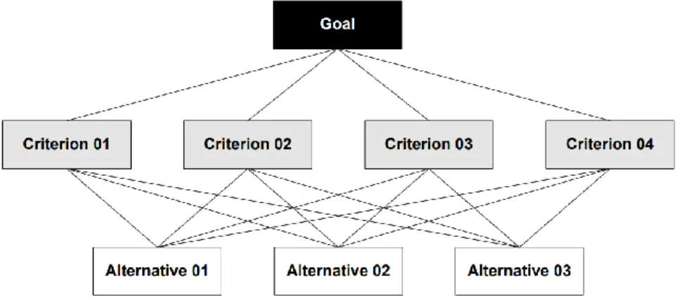
1. Defining the model structure: decomposition means organizing the problem on different levels. A hierarchical structure is built as a decomposition structure that includes the decision goal(s), main criteria, sub-criteria and alternatives to be used to define land suitability levels (Aldababseh et al., 2018). Figure 1. Example of a

(20)

8 hierarchy of criteria An example of decomposition in a hierarchical structure is shown in Figure 1 (Vargas, 2010).

Figure 1. Example of a hierarchy of criteria

2. Standardization of criteria: as was mentioned in section 2.2, a land suitability analysis for urban agriculture dealt with heterogeneous criteria (quantitive/qualitative) that come in different measurement scales. To perform comparative judgments based on expert preferences, it is necessary to convert all criteria into a common domain of measurement. To accomplish this, criteria should be standardized considering the goal and alternatives under evaluation (Prakash TN, 2003).

3. Assigning weights: defining the criterion weights is a fundamental requirement for applying the MCDM/AHP method (Feizizadeh & Blaschke, 2013). A comparison between each criterion under evaluation is carried out based on expert knowledge and literature review to provide the best judgment of their relative importance using a pairwise comparison matrix (Aldababseh et al., 2018). This can be mathematically expressed in the following equation:

𝐴 =[𝑎_𝑖𝑗], 𝑖, 𝑗 = 1, 2, 3 … , 𝑛; (1)

where A is the matrix with 𝑎𝑖𝑗 elements, in which all elements are compared with

themselves, i and j are the criteria with a reciprocity property of 𝑎𝑖𝑗 = 1/𝑎𝑖𝑗 for all

(21)

9

Intensity of importance

Definition Explanation Definition Explanation

1 Equal importance Two activities contribute equally to the objective

3 Weak importance of one _{over another} Experience and judgment slightly favor one activity over _another 5 Essential or strong Experience and judgment strongly favor one activity over _another 7 Demonstrated importance An activity is strongly favored, and its dominance _{demonstrated in practice} 9 Absolute importance The evidence favoring one activity over another is of the _{highest possible order of affirmation}

2, 4, 6, 8

Intermediate values between the two adjacent judgments

2, 4, 6, 8 Intermediate values between the two adjacent judgments

Reciprocals If activity i has one of the above numbers assigned to it when compared with activity j, _{then j has the reciprocal value when compared with i}

Table 1. Scale for pairwise comparisons (T. L. Saaty, 1977)

The level of importance between all criteria is evaluated using Saaty’s s weighting scale shown in Table 1. Weights are estimated by normalizing the pairwise comparison matrix which is obtained by dividing the column elements of the matrix by the sum of each column (Equation 2). Row elements in the obtained matrix are summed, and the total value is divided by the number of elements in the row as is shown in Equation 3:

𝐴’ = [𝑎’_𝑖𝑗], 𝑖, 𝑗 = 1, 2, 3 … , 𝑛 (2) where 𝐴’ is the normalized matrix of A and the 𝑎’𝑖𝑗 is defined as:

𝑎’

_𝑖𝑗

=

𝑎’𝑖𝑗

∑𝑛𝑖=1𝑎𝑖𝑗

(3)

for all i,j = 1, 2, 3, ..., n. Then, criteria weights are estimated as a priority vector or weight vector (Akinci, Özalp, & Turgut, 2013).

𝑤

_𝑖

=

∑ 𝑎’𝑖𝑗 𝑛 𝑗=1

∑𝑛_𝑖=1∑𝑛_𝑗=1𝑎’_𝑖𝑗

(4)

Weights values are within 0 a 1, and their sum is equal to 1

∑

𝑛_𝑖=1

𝑤

_𝑖

= 1

(5) 4. Consistency: A Consistency Ratio (CR) is used to measure the inconsistency obtained as a result of the expert judgments based on the estimation of the

(22)

10 Consistency Index (CI) that validated the consistency in the pairwise comparison matrix (Aldababseh et al., 2018). CI can be estimated and written as:

𝐶𝐼 = (𝜆_𝑚𝑎𝑥− 𝑛) (𝑛 − 1)⁄ (6) where n is the number of elements being compared in the matrix and 𝜆𝑚𝑎𝑥 is the

largest eigenvalue of the matrix. Then, CR is calculated as follows:

𝐶𝑅 = 𝐶𝐼/𝑅𝐼 (7) where RI is the Random index obtained randomly through experiments using samples for different numbers of elements or criteria (Chivasa, Mutanga, & Biradar, 2019). Table 2 shows the RI for the first 10 samples. To be accepted the CR must be < 10%, otherwise, judgments are considered inconsistent and the expert o decision makers should re-evaluate the pairwise comparison to identify the possible inconsistency and repeat the process until the CR could be acceptable. If the CR is below 10%, judgments are considered consistent (T. L. Saaty, 1977).

N 1 2 3 4 5 6 7 8 9 10

RI 0 0 0.52 0.89 1.11 1.25 1.35 1.40 1.45 1.49 Table 2. The Random Indices (T. L. Saaty, 1977).

5. Model Synthesis: suitability scores defined for the sub-criteria or variables (defined in the standardization step) within each criterion are multiplied with the weights assigned for each criterion to calculate the suitability index and generate the final suitability map (Aldababseh et al., 2018).

6. Making a final decision: stakeholders or the decision-makers should come to a final decision with consideration of all important criteria and the results obtained using the AHP method (Fadhil & Moeckel, 2018).

Among many developed multicriteria decision-making methods, this thesis utilized the AHP method because of its capacity to integrate a large amount of heterogeneous data and simplicity to include different opinions (Y. Chen, Yu, & Khan, 2010; Feizizadeh & Blaschke, 2013). Besides, AHP also is widely known among researchers due to its effective mathematical properties and has been implemented in different studies related to

(23)

11 agriculture land-use suitability analysis (Akinci, Özalp, & Turgut, 2013; Montgomery & Schmidt, 2015; Puntsag, Kristjánsdóttir, & Ingólfsdóttir, 2014; Setiawan et al., 2014)

2.3 SENSITIVITY ANALISIS

Decision making is a subjectivity process that is accompanied by uncertainty (Prakash TN, 2003). In the MCDM-AHP method, uncertainty may come from many different sources, such as original data, data processing, criteria selection and judgments of the experts or decision-makers. Experts may not be completely aware of their preferences concerning the criteria or a definition of a unique set of values for the weights is not possible, due to several judgments and preferences coming from multiple experts. The weight estimated for each criterion is one of the most sensitive parameters and a potential contributor to uncertainty in an MCDM - AHP implementation (E. Xu & Zhang, 2013). Therefore, a sensitivity analysis of the weights of input criteria is crucial to reducing uncertainty and increasing the stability of the outputs (Yun Chen, Yu, & Khan, 2013). Sensitivity analysis studies how the variations in input parameters modify the model output (Montgomery & Schmidt, 2015). It can be applied to evaluate how uncertainty in model inputs, influences uncertainty in model predictions. It is considered a good modeling practice to perform validation and calibration of numerical models using sensitivity analysis, to prove the robustness of the final result against small variations in the input data (Crosetto, Tarantola, & Saltelli, 2000).

For the development of this thesis, a combine sensitivity analysis using the One At a Time method (OAT) and GIS techniques was addressed, due to its simple implementation with a low computational cost (Y. Chen et al., 2010). Additionally, the OAT is considered the most straightforward method to validate uncertainty in models, estimating the effect on the evaluation results based on variations in a single input parameter, while holding all other parameters fixed at their nominal values (E. Xu & Zhang, 2013).

(24)

12

2.4 CLASSIFICATION ALGORITHMS

Machine learning techniques are approaches composed of statistical models and algorithms, whose main aim is to learn from the analysis of data (training data) identifying existing patterns and converting this experience into knowledge or expertise to perform a task (Shalev-Shwartz & Ben-David, 2013). There are different categories of machine learning algorithms but usually are classified depending on the learning type (supervised/unsupervised) or learning models (classification, regression, clustering, and dimensionality reduction) or the learning models employed to implement a selected task (Liakos et al., 2018). Random Forest (RF), Support Vector Machine (SVM) and K Nearest Neighbors (KNN) algorithms were selected as they have been implemented as supervised classification models in agriculture land suitability analysis (Heumann et al., 2011; Sarmadian et al., 2014; Senagi et al., 2017). Classification algorithms belong to the category of supervised learning and they are characterized by the use of datasets with labels that generate a predicted class of type discrete (Kuhn & Johnson, 2013)

2.4.1 Random Forest

Random Forest is an ensemble algorithm based on the implementation of multiple decision trees to make classifications and prediction classes (Breiman, 2001). Each tree contains random samples of training data points (from the original data) and each node contains a random subset of predicting variables (features). Additionally, each tree in the forest vote for the classification of a new sample and the final prediction of the algorithm is obtained by the average of votes over the predictions of the individual trees (Kuhn & Johnson, 2013). Due to the construction of ensemble trees, random forest contributes to control variance and overfitting improving the performance of the final prediction (Breiman, 2001). Moreover, it is easy to implement because only two parameters are required: the number of trees (ntree) and the number of predicting variables randomly used (mtry) at each split (Shalev-Shwartz & Ben-David, 2013). The most common way to tune the performance of RF is by increasing the number of decision trees that the algorithm generates to obtain a more reliable result. However, as the final model consists of a group of decision trees, could be difficult to interpret (Castelli, Vanneschi, & Largo, 2019). Figure 2 (Abilash, 2018) shows an example of classification by RF using four trees.

(25)

13

Figure 2. Random Forest classification example of four trees

2.4.2 K - Nearest Neighbors

KNN predicts the label of any new sample based on the labels of the k closest samples from the training set, returning the most common label of the neighbors as the predicted label (Shalev-Shwartz & Ben-David, 2013). “Closeness” is determined by a distance metric, like Euclidean and Minkowski. Therefore, to allow each predictive variable to contribute equally in the distance calculation, centering and scaling are suggested, to avoid any difference in the measurement scale that might affect the resulting distance calculations between samples, generating biased towards predictive variables with larger scales (Kuhn & Johnson, 2013). An example of a 5-nearest neighbor model is depicted in Figure 3 (Kuhn & Johnson, 2013), where a classification of two new samples (denoted by the solid dot and filled triangle) is carried out. Class probability estimates for the new sample are calculated as the proportion of training set neighbors in each class. Therefore, the solid dot sample is near a combination of the two classes where is highly likely that the sample should be labeled as the first class. The other sample is surrounded mostly by neighbors of the second class, hence this one may be labeled as the second class.

(26)

14

Figure 3. The K-nearest neighbor classification model.

2.4.3 Support Vector Machine

The SVM algorithm was designed for binary classification problems (Chiranjit, 2015). SVM aimed to find the hyperplane in the feature space that maximally separates the two target classes (Sarmadian et al., 2014). Therefore, multiple hyperplanes could be chosen, but the one with the maximum margin between data points of both classes would be considered as the best candidate (Chiranjit, 2015). Figure 4 (Gahukar, 2018) shows a case of linearly separable data by hyperplanes, where three possible separating hyperplanes are illustrated. It is evident that the red hyperplane (𝐻3) has a larger margin than the other,

and is, therefore, the best candidate because of its greater generality for classified new data.

(27)

15

Figure 4. Linearly separable data by hyperplanes, where 𝑋1and 𝑋2 are predictive variables, 𝐻1, 𝐻2 and 𝐻3 are hyperplanes, the gray lines are the separation margins and the black and white points represent the two target classes

The major disadvantages of SVM are that including non-informative predicting variables can affect negatively the model and high dimensionality of the feature space increases the computational cost (Kuhn & Johnson, 2013). SVM produces very competitive results and is easy to implement because requires a minimum amount of model tuning (Chiranjit, 2015). The SVM algorithm could be a suitable alternative for the performance of land suitability analysis (Sarmadian et al., 2014).

2.4.4 Model Tuning

Classifications models have parameters that cannot be directly estimated from the data or from an analytical formula, called tuning parameters (Kuhn & Johnson, 2013). For example, in the KNN classification model, the value of K neighbors that the model used to label new samples is a tuning parameter. It is not possible to know in advance which parameter set of values will generate the best model because these parameters do not learn from the data, requiring validation strategies that allow compare different values and select the most adequate for each model (Shalev-Shwartz & Ben-David, 2013). The use of existing data to identify settings for each model parameter allowing to obtain the most realistic predictive performance is called model tuning (Kuhn & Johnson, 2013). K–Fold cross-validation method was selected to implement model tuning due to its

(28)

16 capacity to provide an accurate measure of the true error without wasting valuable data (Shalev-Shwartz & Ben-David, 2013). In this method, the samples of the data are randomly divided into k partitions (folds) of similar sizes and each partition is used to testing a classification model trained to predict the remained samples in the other k-folds (Wong, 2015). The average performance of the hold out partitions is estimated and used to determine the final tuning parameters. A final model is trained using the selected tuning parameters on the entire data set (Kuhn & Johnson, 2013). An example of threefold cross-validation is illustrated in Figure 5 (Kuhn & Johnson, 2013).

Figure 5. A schematic of threefold cross-validation. Twelve data samples are displayed as symbols and allocated in three groups. These groups are left out in turn as models are fit. Performance is estimated from each set of held-out samples and their average would be the cross-validation estimate of model performance.

2.4.5 Model Performance

In Machine Learning, model performance measurement is an important step. Different machine learning models (like regression models) usually implement Root Mean Squared Error (RMSE) and the coefficient of determination ( 𝑅2 _{) metrics to evaluate the}

performance, but in the context of classification models, these metrics are not appropriate to assess the performance (Kuhn & Johnson, 2013). The Area Under the Curve (AUC) of the Receiver Operating Characteristic (ROC) was defined for two-class problems to evaluate the class probabilities of models through a variety of thresholds, indicating how capable the model is at distinguishing between the two classes (de Figueiredo et al., 2018).

(29)

17 Figure 6 shows an example of the ROC curve where the AUC is a measure of the discrimination between two classes always bounded between 0 and 1 (Kuhn & Johnson, 2013). The True Positive Rate (TPR) refers to the ability to correctly identify an event as positive also called sensitivity, and Inversely, the False Positive Rate (FPR) is related to correctly identifying negative events also called specificity (de Figueiredo et al., 2018). The ROC curve plots the TPR and the FPR (one minus the specificity) against each other for each possible threshold. (Pontius & Parmentier, 2014). The model with the highest AUC value would be the best to differentiate the probabilities between the two classes.

Figure 6. Graphic Example of the ROC curve

The AUC - ROC method was selected for measuring model performance in this thesis due to its simple interpretation of class probabilities in classification problems and because of its popularity in evaluating performances and assisting in the decision-making process (de Figueiredo et al., 2018). Additionally, AUC - ROC has been applied for determining the accuracy in similar studies of agriculture land Suitability Analysis using MCDM methods and machine learning techniques (Heumann et al., 2011; Montgomery & Schmidt, 2015; Parthiban & Krishnan, 2016).

(30)

18

3. METHODOLOGY

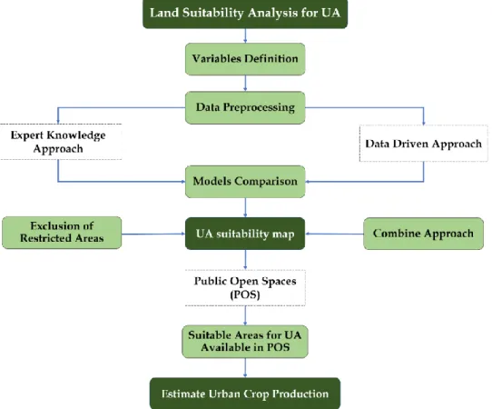
This chapter explains the processes developed for this research. First, the established assumptions in this thesis are mentioned in section 3.1. Then, a description of the software and hardware used is explained in section 3.2, an introduction to the study area and data used is described in section 3.3. The procedure carried out in the expert knowledge approach using the MCDM-AHP method is explained in section 3.4, including a spatial sensitivity analysis developed to evaluate the robustness of the model. The steps implemented in the data-driven approach based on machine learning techniques are explained in section 3.5. Comparison based on the relevant variables in both approaches and the performance of the models implemented is described in section 3.6. Finally, the selection of public buildings and the steps taken to the estimation of public open spaces and crop productivity is presented in section 0. An overview of the methodology implemented is depicted in Figure 7.

(31)

19

3.1 ASSUMPTIONS

The following assumptions were considered for the development of this thesis:

• Although non-food products can be obtained by urban agriculture activities including flowers, aromatic and medicinal herbs, ornamental plants, tree products (seed, wood, fuel, etc.) and tree seedlings (Thomas, 2014). Only vegetable production derived from urban agriculture practices, such as horticulture were considered due to the relevant contributing to food and nutrition security (Orsini et al., 2013).

• City Water can be accessed in every building or household within the city (99.86% coverage) and is suitable to use to grow crops.

• Urban agriculture activities can be developed in indoor and outdoor spaces (Thomaier et al., 2015). The scope of this thesis is oriented only urban agriculture practices in outdoor locations or open spaces.

3.2 SOFTWARE AND HARDWARE

ArcGIS Pro is a GIS application that allows visualizing spatial and attributive

information, performing advanced geoprocessing analysis (ESRI, 2020). Spatial Analyst extension was used to perform the suitability analysis and math and conditional operations based on cell-based raster data (“Spatial analysis in ArcGIS Pro—ArcGIS Pro | ArcGIS Desktop,” 2018)

R is a language for statistical computing and graphics (R Core Team, 2020). It runs on

different operating systems using several packages mostly related to data analysis and visualization. The Integrated Development Environment (IDE) RStudio version 1.1.456 is used as an execution interface of the R software. R version 3.6.1 is used in combination with the following packages:

• ggplot2 (CRAN v. 3.2.1): creates elegant data visualizations using the grammar of graphics (Wickham, 2020). Mainly used for results visualization by creating plots and charts.

(32)

20 • caret (CRAN v. 6.0.84): provides an easy way to create predictive models based on

classification and regression techniques (Kuhn, 2020).

• ROCit (CRAN v. 1.1.1): creates the Receiver operating characteristic (ROC) curve used to measure the performance of Binary Classifier with Visualization

• raster: allows reading, writing, manipulating, analyzing and modeling of raster spatial data (Hijmans, 2020)

Python is an interpreted and object-oriented programming language that due to its

simplicity and readability is used in several research fields (Python.org, 2020). Python version 3.7.0 is used in combination with the following libraries and packages:

• Numpy: library for numerical computations that perform data manipulation and fast mathematical and logical operations on arrays (Van Der Walt, Colbert, & Varoquaux, 2011).

• Arcpy: used for geoprocessing analysis, spatial data manipulation and map automation with Python (Toms, 2015)

• Matplotlib: 2D plotting library for scientific publishing and interactive graphing, used to produce quality graphics (Matplotlib.org, 2020)

Software Applications ArcGIS Pro 2.4.2

Programming Languages Python 3.7.0, R 3.6.1 Integrated Development Environments RStudio, PyScrpter

Data Manipulation Numpy 1.16.3

Data Visualization ggplot2 3.2.1, Matplotlib 3.1.0 Machine Learning Package Caret 6.0-84

CPU Intel(R) Core (TM) i7-6650U 2.20 GHz

Motherboard Microsoft Surface Pro 4

RAM 16 GB DDR4

(33)

21

3.3 DATA AND STUDY AREA

3.3.1 Study Area

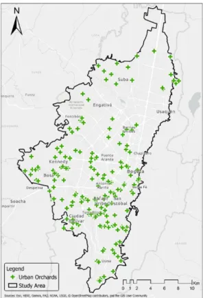
This study focuses on Bogotá city, the capital and the biggest city of Colombia with a latitude of 4° 36' 34.96" north, and longitude of -74° 04' 54.30" west and an altitude of 2.640 m above sea level. The study area is integrated by the urban and urban sprawl areas defined by the urban planning department of the city. Figure 8 shows the location of the study area with an extension of 40.716 Hectares.

Figure 8. Study Area

3.3.2 Data Description

The data used in this thesis is a compendium of different sources obtained by local and governmental entities of the city, which may represent the physical, environmental and socioeconomic components of the study area. Additionally, significant variables for the development of crops and plants in an urban environment were considered based on the received feedback of local experts and similar land suitability studies (Aldababseh et al.,

(34)

22

2018; Feizizadeh & Blaschke, 2013; McClintock et al., 2013; Setiawan et al., 2014; Spataru, Faggian, & Sposito, 2018; Thornton, Momoh, & Tengbe, 2012; Uy & Nakagoshi, 2008a). The term ‘expert’ used in this study, refers to the group of people that due to their academic or professional experience related to urban agriculture contributed with their knowledge in the assessment of the procedures implemented in this thesis. This group is mainly composed of 8 members as shown below:

- The coordinator of the urban agriculture department of the Bogota Botanical Garden

- Two professors with academic knowledge in sustainable agriculture and organic farming

- Two soil scientists with professional experience in agronomy

- One environmental scientist with professional experience of GIS applied to agricultural studies

- Two urban farmers with local knowledge about urban crop production

Although the temperature and different soil properties are vital elements for the development, growth, and productivity of crops in agriculture, being considered relevant variables included in several land suitability analysis; these were not included in this research based on the following criteria:

- Unlike traditional agriculture, urban agriculture is not completely dependent on soil for its development, since it can be created artificially using different methods based on the mixing of organic and inorganic residues to create natural fertilizers that provide the necessary nutrients for the crops.

- The temperature was not considered because this research was not focused on the analysis of a particular agricultural crop, but the identification of potential sites for the specific development of urban cold climate crops native to the study area (Bogota Botanical Garden, 2007).

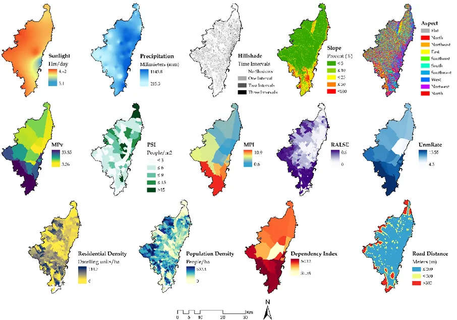
In total fourteen variables were selected and grouped in two main components based on interpretation of literature reviews of internal and external references, availability of data and expert knowledge. Table 4 and Table 5 provide information related to the variables selected for this research, as well as a short definition of each variable, their units, main source-year of the data and their relevance of implementation or study for the UA.

(35)

23 The Bogota Botanical Garden supplied the location in Shapefile format of the current urban orchards in the city (Figure 9). In total, for the study area, there is a record of 202 urban orchards, of which 106 are in private spaces (mainly residential units) and 96 in public spaces (universities, schools, kindergartens, medical centers, etc.). About the type of organization, 79 orchards are managed by communities, 46 by institutions, 23 by schools and 52 by families (Figure 10).

Figure 9. Locations of urban orchards in the study area

(36)

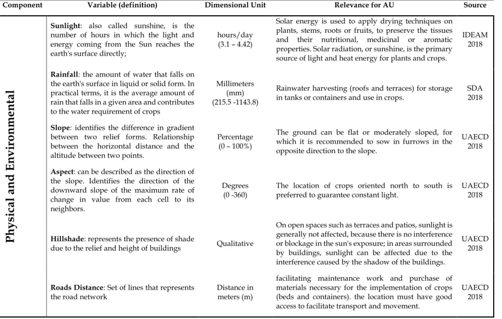
Table 4. Variables description for the physical and environmental component

Component Variable (definition) Dimensional Unit Relevance for AU Source

Ph

ys

ical an

d

En

viron

mental

Sunlight: also called sunshine, is the

number of hours in which the light and energy coming from the Sun reaches the earth's surface directly;

hours/day (3.1 – 4.42)

Solar energy is used to apply drying techniques on plants, stems, roots or fruits, to preserve the tissues and their nutritional, medicinal or aromatic properties. Solar radiation, or sunshine, is the primary source of light and heat energy for plants and crops.

IDEAM 2018

Rainfall: the amount of water that falls on

the earth's surface in liquid or solid form. In practical terms, it is the average amount of rain that falls in a given area and contributes to the water requirement of crops

Millimeters (mm) (215.5 -1143.8)

Rainwater harvesting (roofs and terraces) for storage in tanks or containers and use in crops.

SDA 2018

Slope: identifies the difference in gradient

between two relief forms. Relationship between the horizontal distance and the altitude between two points.

Percentage (0 – 100%)

The ground can be flat or moderately sloped, for which it is recommended to sow in furrows in the opposite direction to the slope.

UAECD 2018

Aspect: can be described as the direction of

the slope. Identifies the direction of the downward slope of the maximum rate of change in value from each cell to its neighbors.

Degrees (0 -360)

The location of crops oriented north to south is preferred to guarantee constant light.

UAECD 2018

Hillshade: represents the presence of shade

due to the relief and height of buildings Qualitative

On open spaces such as terraces and patios, sunlight is generally not affected, because there is no interference or blockage in the sun's exposure; in areas surrounded by buildings, sunlight can be affected due to the interference caused by the shadow of the buildings.

UAECD 2018

Roads Distance: Set of lines that represents

the road network

Distance in meters (m)

facilitating maintenance work and purchase of materials necessary for the implementation of crops (beds and containers). the location must have good access to facilitate transport and movement.

UAECD 2018

(37)

25

Component Variable (definition) Dimensional Unit Relevance for AU Source

Soci

al

and

E

co

n

omi

c

Public Space Indicator (PSI): establishes the

relationship between Effective Public Space (public space of a permanent nature, made up of green areas, parks, squares, and small squares) and the population

People/m2 (< 3; 3 – 6; 6 – 9;

9 – 15; > 15)

Representative parks, green areas, or small squares in public spaces that could represent potential places for the establishment of AU practices.

DADEP 2018

Population Density: the ratio of the number of people

per hectare

People/ha (0 – 633.4)

Identify areas where a greater number of people located in residential properties and housing units can benefit from implementing AU practices

SDP 2018

Residential Density: the ratio of the number of

dwelling units per hectare

Dwelling units /ha (0 -114.7)

UAECD 2018

Dependency Index: relationship between the

dependent people, (<15 and >64 years), and the population in working age (≥15 and 64 years). The data shows the ratio of dependents per 100 persons of working age.

Index (31.58 – 50.12)

Identify zones with low socioeconomic levels, extreme poverty, nutritional and food problems within the study area, to focus efforts on the establishment of possible scenarios that contribute to improving food and nutritional security by implementing AU practices

DANE 2017

Multidimensional Poverty Index (MPI): identifies

multiple deprivations at the household and individual level in health, education, and standard of living

Index (0.6 – 10.9)

DANE 2017

Monetary Poverty (MPv): percentage of the population

with income below to the minimum monthly income defined as necessary to meet their basic needs

Percentage (3.06 – 33.85)

DANE 2017

Unemployment Rate (UmpRate): relationship between

the unemployment people and the working population

Rate (4.3 – 13.55)

DANE 2017

Residential Areas with Low Socioeconomic Level (RALSE): weighting of properties for residential use

classified with low economic levels according to their socioeconomic stratification

Index (0 – 0.6)

DANE 2017

Table 5. Variables description for the social and economic component

- UAECD – Unidad Administrativa Especial de Catastro Distrital; DANE - Departamento Administrativo Nacional de Estadística; SDP - Secretaría Distrital de Planeación; DADEP - Departamento Administrativo de la Defensoría del Espacio Público; SDA - Secretaría Distrital de Ambiente; IDEAM - Instituto de Hidrología, Meteorología y Estudios Ambientales

(38)

3.3.3 Data Preparation

Aspect and Slope layers were obtained from a DTM of 5m resolution. The hillshade layer required a more extensive preprocessing. It was necessary to identify areas would be most affected by shadows during the day due to the presence of buildings around. To do this the following steps were implemented:

- Buildings height was estimated by selecting the dwelling units and multiplying the number of floors by 2.5 m (average height of a residential floor in the city of Bogota) and for the rest of the buildings, a value of 3m was used for height estimation.

- A raster layer was created using the estimated building's height and added to the DTM cell values.

- Hillshade maps were created for three periods of time in the day, the morning time (8 am), midday (12 pm) and afternoon (4 pm) using the average values of the azimuth and elevation of the first day of each month for 2018.

- A final hillshade composes map was created for the study area identifying areas that would not be affected by shadows during the day and areas that would be affected in one, two or three periods of time during the day.

Finally, all variables were adjusted to the extent of the study area and converted into raster layers at a spatial resolution of 5m which is the coarsest resolution of the available spatial layers. Figure shows the result of the variables after the processes mentioned in this section.

(39)

Figure 11. Variables selected for the study area. MPI (Multidimensional Poverty Index); UnmRate (Unemployment Rate); PSI (Public Space Indicator); Mpv (Monetary Poverty); RALSE (Residential Areas with Low Socioeconomic Level)

(40)

3.4 EXPERT KNOWLEDGE APPROACH: MCDM - AHP METHOD

This approach aims to define land suitability for urban agriculture in the study area, combining the potential of spatial data manipulation and analysis provide by GIS techniques with MCDM using the AHP method. Knowledge, support, and feedback from the experts are fundamental during the development of this method, in which, most of the procedures require their participation except for the steps developed within the GIS environment as can be seen in Figure 12.

Figure 12. Flowchart of the land suitability map for urban agriculture based on expert knowledge approach

3.4.1 Defining Land Suitability Classification for Urban Agriculture

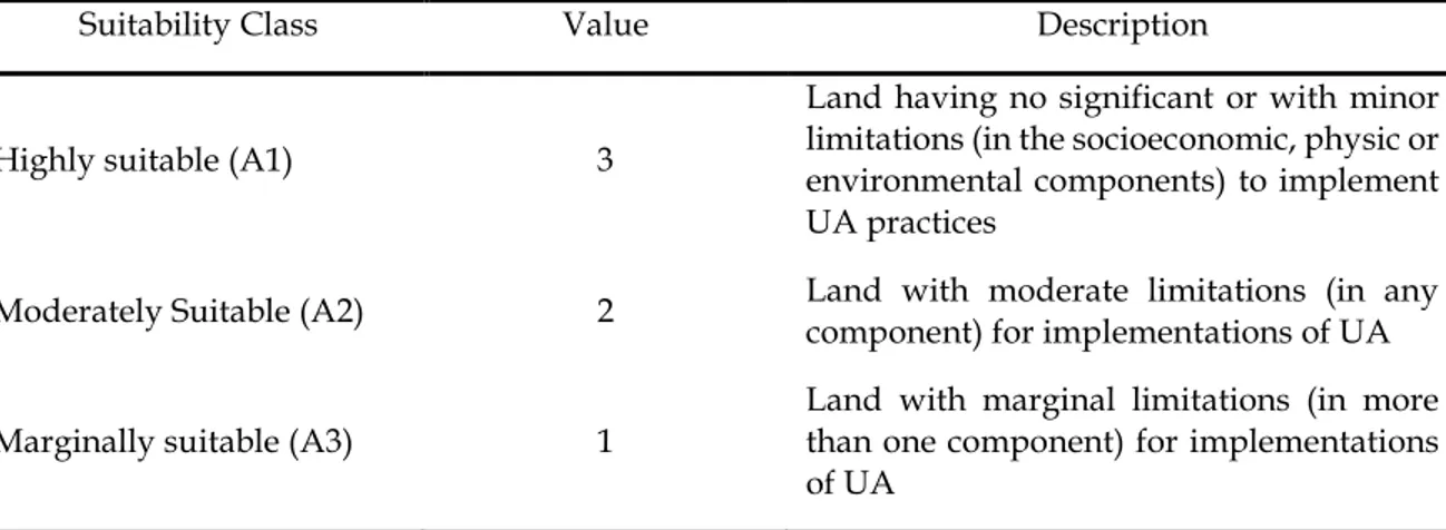
Land evaluation is a process that allows the identification and assessment of specific uses that are adapted to specific conditions of the land assessed (FAO, 2007). Although the FAO (Food and Agriculture Organization) system presents some limitations because of its orientation mainly on the physical aspect, it has been the most widely used procedure to address local, regional land management. FAO framework proposes a set of qualities and characteristics to be used in the land evaluation process (called in this research as criteria and variables, respectively) where the number is flexible and usually is determined by the objectives of the study, the scope of the research and the data available

(41)

29 (FAO, 2007). The classification system used in this thesis was inspired by the FAO approach dedicated to sustainable agriculture, where suitability is a measure of how well the qualities of a land unit match the requirements of a particular form of land use. For this research, the land suitability for urban agriculture was classified into three main categories ranging from most or highly suitable to marginally suitable based on the contribution to the alleviation of urban poverty by increasing food security and nutrition in the study area Table 6.

Suitability Class Value Description

Highly suitable (A1) 3

Land having no significant or with minor limitations (in the socioeconomic, physic or environmental components) to implement UA practices

Moderately Suitable (A2) 2 Land with moderate limitations (in any component) for implementations of UA

Marginally suitable (A3) 1

Land with marginal limitations (in more than one component) for implementations of UA

Table 6. Land Suitability Classification and Definition Used for Urban Agriculture

3.4.2 Building a Hierarchical Structure

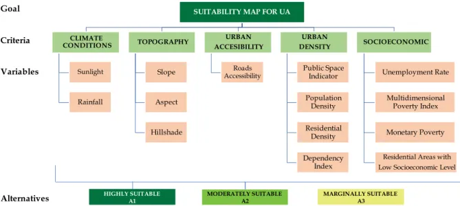
A decomposition process was built in a hierarchical structure where the overall objective was to obtain a land suitability map for UA, including the criteria and variables used to define land suitability. In total, five main criteria were defined: climate conditions, topography, urban density, urban accessibility and socioeconomic. Subsequently, the decomposition continues to define the variables under each one of these five main criteria. The resulting hierarchal structure is shown in Figure 13.

(42)

30

Figure 13. Hierarchal structure for defined land suitability for UA

The purpose of this procedure is to identify certain factors that affect the suitability of the land, which can be quantified in a specific range of values. For example, it is not easy to estimate numerically how climate conditions affect land suitability in general. However, when it is decomposed in a decision tree into sunlight and rainfall variables, each of these variables can be easily quantified to provide a more feasible approximation (Aldababseh et al., 2018). An example of a decision tree for the climate conditions criteria is depicted in Table 7. Decision tree tables for the other criteria can be found in Appendix A.

Sunlight

(hours/day) Precipitation (mm) Suitability Class

≥ 4 ≥ 500 A1 < 500 A2 ≥ 3.5 - < 4 ≥ 500 A2 < 500 A3 < 3.5 ≥ 500 A3 < 500 A3

Table 7. Climate conditions criteria decision tree

Sunlight ainfall Slope Aspect illshade oads Accessibility Public Space Indicator Population ensity esidential ensity ependency Index nemployment ate ultidimensional Poverty Index onetary Poverty

esidential Areas with

ow Socioeconomic evel

(43)

31

3.4.3 Standardization of the Criteria

Evaluation criteria in land suitability analysis are represented by qualitative values or classes, indicating the degree of suitability which will be represented in the final suitability map (Prakash TN, 2003). The variables selected for the study were classified in suitability classes (A1, A2, and A3) according to the values defined in Table 8 using the reclassify tool located in ArcGIS Pro. Based on the decision trees defined in the hierarchical structure, the variables were combined using the combine tool located in ArcGIS Pro to conformed the five main criteria. Then, suitability classes were rated to define their relative importance in the main criteria and to establish numerically how these would contribute to the final suitability map. Therefore, values in Table 6 were used to rate the classes for the five main criteria. Figure 14 shows an example of the standardization process for the climate conditions criteria.

Figure 14. Standardization process for climate conditions criteria

3.4.4 Assessing the Weights and Consistency

A pairwise comparison matrix where the five main criteria were compared with themselves was constructed using Saaty’s scale measurement (Table 1) to assign the relative importance of one criterion over one another. Criterion weights were estimated using the eigenvector corresponding to the largest eigenvalue of the matrix (𝜆𝑚𝑎𝑥) and

then normalizing the sum of the components. With the weights defined the next step is to check the consistency of the pairwise comparison matrix obtained. Using 𝜆𝑚𝑎𝑥

estimated previously and a Random Index equivalent to the five criteria, the Consistency Index (CI) and subsequently the Consistency Ratio (CR) were estimated to validate the consistency of the matrix, indicating if the values for criteria comparison were assigned randomly. 2 1 5 8 1800 50 A1 A2 A1 A1 A A A2 A1 A 1 2 Sunlight ainfall

limate onditions limate onditions

(44)

Criteria Variable Dimensional Unit UA Suitability Class Highly Suitable (A1) Moderately Suitable (A2) Marginally Suitable (A3) P h ysi ca l & E n vironm en ta l Climate Conditions Sunlight hours/day (3.1 – 4.42) ≥ ≥ 3.5 - < 4 < 3.5 Rainfall Millimeters (mm) _{(215.5 -1143.8)} ≥ 500 <500 - Topography Slope Percentage _{(0 – 100%)} ≤ 25 > 25 - ≤ 50 > 50 Aspect Degrees _{(0 -360)} North (0–22.5; 337.5–360) South (112.5–247.5) West 22.5–112.5 - East 247.5–337.5 -

Hillshade _{(Presence of shadows)}Qualitative No Shadows Once or Twice times _{per day} Three times per _day

Urban

Accessibility Roads Distance Meters (m) ≤ 200 > 200 - ≤ 500 > 500

S oci al & E con omi c Urban Density

Public Space Indicator (PSI) People/m² ≥ 6 ≥ - < 6 < 3

Population Density People/ha ≥ 200 ≥ 100 - < 200 < 100

Residential Density Dwelling units/ha ≥ 25 ≥ 5 - < 25 < 5

Dependency Index _{(31.58 – 50.12)}Index ≥ 5 ≥ 0 - < 45 < 40

Socioeconomic

Multidimensional Poverty Index (MPI)

Index

(0.6 – 10.9) ≥ 5 ≥ - < 5 < 3

Monetary Poverty (MPv) Percentage

(3.06 – 33.85) ≥ 20 ≥ 10 - < 20 < 10

Unemployment Rate (UmpRate)

Rate

(4.3 – 13.55) ≥ 10 ≥ 5 - < 10 < 5

Residential Areas with Low Socioeconomic Level (RALSE)

Index

(0 – 0.6) ≥ 0.4 ≥ 0 2 - < 0.4 < 0.2

Land suitability analysis to assess the potential of public open spaces for urban agriculture activities