Universidade do Minho
Escola de Engenharia Departamento de Informática
João Miguel Afonso
Towards an Efficient OLAP Engine
based on Linear Algebra
Universidade do Minho
Escola de Engenharia Departamento de Informática
João Miguel Afonso
Towards an Efficient OLAP Engine
based on Linear Algebra
Master Dissertation
Master Degree in Computer Science
Dissertation supervised by
Alberto José Proença José Nuno Oliveira
A C K N O W L E D G E M E N T S
This work was financed by the ERDF – European Regional Development Fund through the Operational Programme for Competitiveness and Internationalisation - COMPETE 2020 Programme within project «POCI-01-0145-FEDER-006961», and by National Funds through the Portuguese funding agency, FCT - Fundação para a Ciência e a Tecnologia as part of project «UID/EEA/50014/2013».
I would like to express my deep gratitude to Professor Alberto Proença and Professor José Oliveira, my research supervisors, for their patient guidance, enthusiastic encouragement and useful critiques of this work.
To Bruno Ribeiro, João Fernandes, Gabriel Fernandes, Fernanda Alves, Filipe Oliveira, and Rogério Pontes, for their previous contributions in the project. More specially to João, with whom I worked together in (Afonso and Fernandes,2017), and to Bruno, for always
contributing with new ideas to implement the vision we all worked for.
Finally, to my family, whose continuous support has been essential to overcome the mul-tiple obstacles I found during the way.
A B S T R A C T
Relational database engines associated to the widely used Structured Query Language (SQL) are suffering unsatisfactory performance results in complex business queries, due to ever increasing volumes of stored data. To retrieve and process data in a more efficient way, Online Analytical Processing (OLAP)models have been proposed with an increased focus on attributes (measures and dimensions) over records.
OLAP is based on a row-oriented theory, while a columnar-oriented theory could con-siderably improve the performance of analytical systems. TheTyped Linear Algebra (TLA)
approach is an example of such theory: it encodes each database attribute in a distinct ma-trix. These matrices are combined in a single Linear Algebra (LA)expression to obtain the result of a query.
This dissertation combines concepts of relational databases,OLAP,TLAand performance engineering to design, implement and validate an efficientTLA-DB engine:SQLqueries are converted into its equivalent LAexpression, using Type Diagrams (TDs), which represent each matrix as an arrow pointing from the number of columns to the number of rows,TDs
are converted to a LAexpression encoded in Linear Algebra Query language (LAQ) and theLAQscript of a query is automatically coded inC Plus Plus (C++).
An efficientTLA-DB engine required the encoding of the sparse matrices in an adequate format, namely Compressed Sparse Column (CSC), while the operations specified inLAQ
expressions had their performance improved by optimised algorithms and an optimised query processor.
The functionality of the resultingLAQengine was validated with severalTPC Benchmark H (TPC-H)queries for various dataset sizes. A comparative evaluation of theTLA-DB with two popular Database Management Systems (DBMSs), PostgreSQL and MySQL, showed that the developed framework outperforms bothDBMSsin mostTPC-Hqueries.
R E S U M O
As melhorias de desempenho dos sistemas de gestão de bases de dados relacionais não têm sido suficientes para acompanhar o crescimento do volume de dados com que são utilizados. Para colmatar a consequente necessidade de soluções mais eficientes, a teoria
OLAP foi proposta. Esta introduz as noções de medidas e dimensões, guardando pré-agregações das medidas baseadas nas últimas, de forma a acelerar o processo de análise de dados.
Contudo, ainda que com regras mais restritas, oOLAPestá assente em álgebra relacional. A proposição de uma teoria orientada à coluna pode abrir portas a grandes melhorias de desempenho em consultas analíticas. A álgebra linear tipada é um bom exemplo. Segundo esta teoria, cada um dos atributos é convertido numa matriz independente, as quais são pos-teriormente combinadas através de uma expressão de álgebra linear que define o resultado da consulta.
Esta dissertação combina conceitos de bases de dados relacionais, OLAP, álgebra lin-ear, teoria de tipos, e computação eficiente para projetar, implementar e validar um motor
OLAP robusto e eficiente. Para tal, consultas emSQLsão convertidas para a expressão de álgebra linear equivalente, usando diagramas de tipo que representam cada matriz como uma seta a apontar do número de colunas para o número de linhas da matriz. A expressão que deles resulta é então codificada emLAQe automaticamente implementada emC++.
Para garantir a eficiencia da ferramenta desenvolvida, todas as matrizes foram guardadas num formato adequado, nomeadamente o CSC. Por sua vez, as operações especificadas na
LAQforam implementadas recorrendo a algoritmos optimizados.
A correção do sistema implementado foi garantida através da validação dos resultados de um grupo de consultas extraidas doTPC-H, executadas sobre bases de dados de multiplos tamanhos. Finalmente, a comparação com dois sistemas de bases de dados convencionais (o PostgreSQL e o MySQL) nas métricas de tempo de execução e memória utilizada, demon-strou a maior eficiencia da ferramenta desenvolvida na maioria das consultas.
C O N T E N T S
1 i n t r o d u c t i o n 1
1.1 The Relational Model 2
1.1.1 Relational Algebra 3
1.1.2 SQL 3
1.2 Database System Implementation 6
1.2.1 Query Compilation 6
1.2.2 Query Execution 9
1.3 Data Warehousing 10
1.3.1 Data Modeling 11
1.4 Challenges & Goals 12
1.5 Contribution 13
1.6 Dissertation Outline 13
2 t y p e d l i n e a r a l g e b r a f o r o l a p 14
2.1 Linear Algebraic Encoding of Data 14
2.1.1 Dense Vectors 14
2.1.2 Sparse Matrices 15
2.2 Type Diagrams 15
2.3 Linear Algebra Query language 16
2.3.1 Dot Product 17 2.3.2 Khatri-Rao Product 18 2.3.3 Hadamard-Schur Product 18 2.3.4 Filter 19 2.3.5 Fold 20 2.3.6 Lift 20 2.4 Conversion algorithm 21 2.4.1 The approach 21 2.5 Conversion Example 27 2.6 Summary 32
3 a t l a-db engine for relational sql 33
3.1 Matrix Representation 33 3.1.1 LIL 34 3.1.2 COO 35 3.1.3 CSC/CSR 35 3.1.4 Matrix labels 38 iv
Contents v 3.2 LA Operators 38 3.2.1 Hadamard-Schur Product 39 3.2.2 Khatri-Rao Product 39 3.2.3 Dot Product 43 3.2.4 Filter 44 3.2.5 Fold 45 3.2.6 Lift 46 3.3 “Streaming” approach 46
3.3.1 Dependencies in query processing 46
3.3.2 Execution order 47 3.4 SQL Driver 48 3.4.1 SQL Parser 48 3.4.2 Query Rewriter 49 3.4.3 SQL Converter 49 3.4.4 toString 50 3.5 LAQ Engine 50 3.5.1 LAQ Parser 50 3.5.2 Query Optimiser 51 3.5.3 Query Processor 51 3.5.4 Run-time Compiler 54 3.5.5 Query Execution 54
3.6 The framework manager 55
3.7 Summary 55
4 va l i d at i o n a n d p e r f o r m a n c e r e s u lt s 56
4.1 TPC Benchmark H 56
4.1.1 Benchmark modifications 57
4.2 Testbed environment 58
4.3 Results and discussion 59
4.4 Summary 63 5 c o n c l u s i o n s 64 5.1 Future work 66 5.1.1 Framework extensions 66 5.1.2 Horizontal scalability 70 5.1.3 Incremental querying 72
a t p c-h queries - sql and laq versions 76
a.1 Query 3 76
Contents vi
a.3 Query 6 78
a.4 Query 11 78
a.5 Query 12 79
L I S T O F F I G U R E S
Figure 1 TPC-H Query 3 – Relational Algebra representation 7
Figure 2 TPC-H Query 3 – RA optimized representation 8
Figure 3 System architecture 33
Figure 4 Detailed system architecture 34
Figure 5 A sparse matrix in CSC format 36
Figure 6 TPC-H query 6 - execution plan 48
Figure 7 TPC-H database schema 57
Figure 8 TPC-H queries 3 and 6 – preliminary performance results 59
Figure 9 TPC-H queries 3 and 4 performance results 60
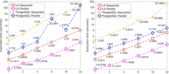
Figure 10 Execution times (scale factor: 25) 61
Figure 11 Sequential and Parallel Query 6 62
Figure 12 Memory usage (scale factor: 25) 62
Figure 13 TPC-H queries 3 and 4 performance results (MonetDB) 69
Figure 14 Execution times (scale factor: 25) 69
Figure 15 Memory usage (scale factor: 25) 69
Figure 16 Distributed dot product - replicate A 70
Figure 17 Distributed dot product - rotate A 71
L I S T O F TA B L E S
Table 1 Relational Model terminology 2
Table 2 TPC-H relation Lineitem 2
Table 3 TPC-H relation Orders 2
Table 4 Relational Algebra operators 4
Table 5 OLTP vs Data Warehousing systems 11
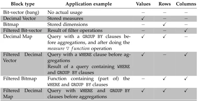
Table 6 Properties of CSC block types 37
Table 7 Testbed environment 59
A C R O N Y M S
A
ALAggregations List. 4
APIApplication Programming Interface. 52,55 B
BIBusiness Intelligence. 1 C
C++C Plus Plus. ii,iii,13,51,54,55,65
CBLAS C language Basic Linear Algebra Subprograms.38,45,64 CFGContext-Free Grammar. 21,50,68
COOCoordinate List. 34–36,64,67 CRUDCreate Read Update Delete. 10
CSCCompressed Sparse Column. ii,iii,34–36,40,42,43,46,64,67 CSRCompressed Sparse Row.34,35,64
CSVcomma-separated values.34 D
DBMSDatabase Management System. ii,1,6,12,13,38,48,54,56,58,60,62,65–67 DCL Data Control Language. 3
DDLData Definition Language. 3 DMLData Manipulation Language. 3 DQLData Query Language. 3
DSLDomain Specific Language. 14,16,32,64 DTLData Transaction Language. 3
DWData Warehouse. 11 G
GA Grouping Attributes. 4 GMPGNU Multi Precision. 65 I
Acronyms x
IDCInternational Data Corporation. 1
Intel MKLIntel Math Kernel Library. 38,45,64 L
LALinear Algebra. ii,12–14,16,21,27,31–33,38,51,55,57,58,60–67,69,70
LAQ Linear Algebra Query language. ii,iii, 13, 16, 21, 27, 31,33, 37, 38, 45–47, 49–53,55, 58,60,64–66,68,70,72
LIL List of Lists.34,35,64 O
OLAP Online Analytical Processing.ii,iii,11,12,16,21,32,45,56,65,68 OLTPOnline Transaction Processing. 10,11
OSOperating System. 67 P
PUProcessing Unit.59,61 R
RARelational Algebra. 3,5,6,12,21,22 RAMRandom Access Memory. 58,59,62,63 RCRelational Calculus. 3
RDBMSRelational Database Management System.2,33,49,69 RMRelational Model. 1,2
S
SQLStructured Query Language. ii,iii,1, 3, 5,6, 9, 12–14, 16, 20, 21, 23,26–28, 32, 33,37, 45,48–50,53,55,56,58,65,66,68
T
TDType Diagram. ii,15–17,19,20,23,28,32,49,65,68 TLATyped Linear Algebra. ii,13,14,32,49
TPCTransaction Processing Performance Council. 56 TPC-DSTPC Benchmark DS. 56
TPC-HTPC Benchmark H. ii,iii,2,21,47,50,56,57,59,60,63,65,68,72 TSVtab-separated values. 34
1
I N T R O D U C T I O N
“From paper-based files to the electronic era, there is not one aspect of modern business that has avoided the need to collect, collate, organise and report upon data” Lake and Crowther(2013).
The importance of data in the business context is unquestionable, and the amount of electronic data that companies have in hand is growing exponentially, developing the ideal environment for high profits.
However, a study developed by the International Data Corporation (IDC) (Gantz and Reinsel,2012) revealed that only 0.5% of this data is actually analysed. This slight
percent-age reveals that the improvements in data processing systems and methodologies are not enough to compete with the data growing rate.
In fact, the development of a DBMS is certainly among the most complex projects in computer science. Not only all the theoretical basis must be carefully and extensively researched, but all the system components must be efficiently implemented and tested under a wide range of queries and datasets.
It is true that many recent systems have been built for more special purpose tasks, slightly bypassing the establishment of a formal basis. But is also true that most of these systems have failed to compete with the standard solutions.
The best example is probably Map-Reduce. Purposely built in 2005 to support Google’s crawl database, it was replaced a few years later by Big Table, and only now the world is realising that even a software built by Google can have no practical applicability ( Stone-breaker et al.,2015, p. 4).
Still in the same mindset, the basis of all major system is, or is prone to become, relational
SQL(Stonebreaker et al.,2015, p. 5). Considering that the relational theory has been on the
market for almost fifty years, and is still the standard approach to databases is the proof that formal theories tend to support the development of better software.
The next sections introduce the reader the key issues in the evolution of database systems, from Codd’s Relational Model (RM) to modern implementations considering Business In-telligence (BI)methodologies. This context is relevant to better comprehend the core topics addressed by this work.
1.1. The Relational Model 2
1.1 t h e r e l at i o na l m o d e l
In his paper “A Relational Model of Data for Large Shared Data Banks” (Codd, 1970), Edgar
Codd proposed the database model which would become the theoretical foundation of all
Relational Database Management Systems (RDBMSs)(Connolly and Begg,2014, p. 149).
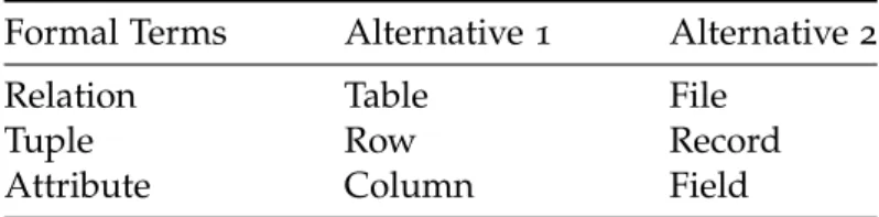
As a result of the successive adjustments in these systems and the subsequent deviations from the original model, the terminology of theRMis quite confusing. Some concepts have multiple designations, so a short summary is presented in Table1.
Formal Terms Alternative 1 Alternative 2
Relation Table File
Tuple Row Record
Attribute Column Field
Table 1.: Relational Model terminology. Based onConnolly and Begg(2014, p.154)
As the name suggests, the RM is based on the mathematical concept of relation. Re-lations serve to keep all the information stored in the database. They are represented as bi-dimensional tables in which the rows of the table correspond to individual records (tu-ples) and the table columns correspond to attributes (Connolly and Begg,2014, p. 152).
For example, the Tables2and3respectively depict the relations Lineitem and Orders.
An-alyzing the tables, one can identify that the relation Lineitem is composed by the attributes Quantity and OrderKey, while the relation Orders incorporates the attributes OrderKey, Or-derDate and ShipPriority. Furthermore, the cardinality (number of records) of both relations is the same. Lineitem Quantity OrderKey 28 32 44 32 13 34
Table 2.: TPC-H relation lineitem1
Orders
OrderKey OrderDate ShipPriority 32 1995-07-16 1-URGENT 33 1993-10-27 2-HIGH 34 1998-07-21 1-URGENT Table 3.: TPC-H relation orders1
The RM states that there can be no duplicate tuples within a relation. To ensure this property, it is necessary to properly identify each tuple of the relation with a primary key. This key is an attribute (or set of attributes) from the relation where all the records are distinct.
1 To maintain the document consistency, all the database examples used in this dissertation are based onTPC-H. This benchmark will be described in section4.1.
1.1. The Relational Model 3
When an attribute exists in more than one relation, it usually represents a relationship between tuples of the two relations (Connolly and Begg, 2014, p. 159). For example, the
inclusion of OrderKey in both Orders and Lineitem relations connects each order to the items that compose it. In the Orders relation, OrderKey is the primary key. However, in the Lineitem relation, the OrderKey attribute is a foreign key.
These keys are extremely important because they are the only way of relating information spread across multiple tables. The law of referential integrity specifies that every non-null value in a foreign key must match a primary key value of some tuple in its home relation (Connolly and Begg,2014, p. 162).
1.1.1 Relational Algebra
More than the definition of a structure for the database and its data, any database model must specify a set of operations on the information stored in the database (Connolly and Begg, 2014, p. 93). To fulfill this purpose,Codd(1971) introduced Relational Algebra (RA)
and theRelational Calculus (RC).
As defined byConnolly and Begg(2014, p. 168), “The relational algebra is a theoretical
lan-guage with operations that work on one or more relations to define another relation without changing the original relation(s)”. This type similarity between the input and output of relational ex-pressions allows their composition in an analogous way to arithmetic operations.
There are five key operations inRA: selection, projection, Cartesian product, union and set difference. Based on them, other operations have been defined, for example the join and intersection,Connolly and Begg(2014, p. 168).
Both RA and RC are too broad to be exhaustively described in this document. Table
4 contains a summary of the enumerated operations, based on Connolly and Begg (2014,
pp. 169–180). Please consultConnolly and Begg(2014) and Molina et al.(2008) for further
information.
1.1.2 SQL
RAis a mathematical language, difficult to use in database manipulation tasks. To achieve a higher level of abstraction and facilitate this tasks, other RAbased languages have been proposed, beingSQL one of them.
TheSQLlanguage can be divided in five major groups: Data Definition Language (DDL),
Data Manipulation Language (DML),Data Query Language (DQL),Data Control Language (DCL), andData Transaction Language (DTL). The present analysis will be summarised and restricted to theDQL, more specifically to the SELECT statement.
1.1. The Relational Model 4
Selection(σpredicate(R))- an unary operation with a single relation (R) that produces a relation containing only those tuples of R that satisfy the specified condition (predi-cate).
Projection(πa1,...,an(R))- an unary operation that produces a relation containing a vertical subset of R with the specified attributes and eliminating duplicate tuples.
Union(R∪S)- a binary operation that produces a relation containing all tuples of R and S, without duplicate tuples. R and S must be union-compatible.
R ∪ S R
S
Set difference(R−F)- produces a relation with all tuples in R that do not exist in S. R and S must be union-compatible.
R − S R
S
Intersection(R∩S)- produces a relation containing all tuples present in both R and S. R and S must be union-compatible.
R ∩ S R
S
Cartesian product (Cross Join)(R×S)- produces a relation that is the concatenation of every tuple of relation R with every tuple of relation S.
A a b × B 1 2 3 = A B a 1 a 2 a 3 b 1 b 2 b 3 Theta join(R./FS)- produces a relation that contains tuples satisfying the predicate F from the Cartesian product of R and S, that is, R./FS=σF(R×S). The resultant predicate is of the type RattributeθSattribute, where θ must be a comparison operator: <,>,≤,≥,=,6=
Equijoin(R./FS)- similar to theta join, produces a relation that contains tuples satisfying predicate F, while restricting the comparison operators to equality, Rattribute=Sattribute.
Natural join (R ./ S) - equivalent to an equijoin of two relations over all common attributes. Only a single occurrence of each attribute is kept. As illustrated, the natural join of the Tables2and3with abbreviated attribute names.
Lineitem./Orders Q OK OD SP 28 32 1995-07-16 1-URGENT 44 32 1995-07-16 1-URGENT 13 34 1998-07-21 1-URGENT
(Right) Outer join(R|><|dS) - a natural join where tuples from S that do not match any values in the common attributes of R are also included in the output relation. The presented table contains the right outer join of the Tables2and3(Lineitem and
Orders). Lineitemd|><|Orders Q OK OD SP 28 32 1995-07-16 1-URGENT 44 32 1995-07-16 1-URGENT 33 1993-10-27 1-URGENT 13 34 1998-07-21 1-URGENT
Semijoin(R.FS)- operates on the relations R and S, producing a relation that includes only attributes from R. The obtained tuples are the ones in R that participate in the join of R with S, satisfying predicate F. This way, R.FS=πA(R./FS)
Lineitem . Orders Quantity OrderKey
28 32 44 32 13 34 Aggregate(AL(R))- applies anAggregations List (AL)to the relation R, defining a new relation with the results of the aggregations. ALcontains one or more pairs of attributes and aggregate functions, e.g., SUM, COUNT, AVG, MIN and MAX.
Grouping (γGA AL(R), as in Molina et al. (2008, p. 778)) - groups the tuples of R by the Grouping
Attributes (GA). The values in each created group are then combined with the aggregation operators specified inAL. The output relation contains theGA, along with the results of all the aggregate functions.
1.1. The Relational Model 5
The SELECT statement aims to retrieve data from the database, being the most usedSQL
command. As explained by Connolly and Begg(2014, p. 197), the basic structure of this
instruction is the following:
SELECT [DISTINCT | ALL] {* | [columnExpression [AS newName]] [,...]}
FROM TableName [alias] [,...]
[WHERE condition]
[GROUP BY columnList] [HAVING condition] [ORDER BY columnList]
It has two mandatory clauses: SELECT and FROM and three optional ones: WHERE, GROUP BYand ORDER BY.
The SELECT statement is similar to the relational projection, although the selected at-tributes are kept intact, that is, the repeated tuples are not removed. The atat-tributes con-tained in this clause can be involved by an aggregation function.
The FROM clause is the simplest one, because it just enumerates the tables that will be used in the query. Using the presented syntax the table joins are always implicit, avoiding the inclusion of multiple statements : [INNER | [LEFT | RIGHT | FULL] [OUTER]] JOIN. All of them can be recreated by combining implicit joins and WHERE clauses.
The WHERE statement corresponds to theRAselection operation, being used to restrict the rows to be retrieved. It must be followed by a condition (or predicate), used to filter the desired records. Connolly and Begg(2014, p. 201) specifies five basic conditions:
1. The direct comparison of two expressions, e.g. a≥b;
2. The value of an expression is within a defined range, e.g. a BETWEEN(x, y);
3. The value of an expression equals an element in a set, e.g. a I N(x, y, ...), where x, y, ... can be tuples with one or more elements;
4. The value of an expression matches a predefined pattern, e.g. a LIKE “pattern” 5. The value is null.
Corresponding to the relational grouping operator, the GROUP BY clause can be used to calculate sub-aggregations of data, based on the similarity of records extracted from a spec-ified set of columns.
However, for the SQL query to be valid, the GROUP BY and the SELECT clauses must be integrated under some rules. For example, all attributes in the SELECT statement must either be present in the GROUP BY clause or be involved by an aggregation function (Connolly and Begg,2014, p. 210).
The ORDER BY clause is self explanatory, simply sorting the records based on the specified attributes.
1.2. Database System Implementation 6
Although the presented structure of the SELECT only represents a narrow view of the command, it can be used to describe most of theSQLqueries.
1.2 d ata b a s e s y s t e m i m p l e m e n tat i o n
One of the main goals when designing user-friendly applications is to guarantee short response times. In the database environment, this translates to a demand for real-time query processing of always increasing volumes of data.
To pursue this objective,DBMSdevelopers had to consider performance in high priority, optimizing all critical components of a system. However, considering that the algorithms to be executed are strongly tied to eachSQLquery, a less efficient implementation can lead to hours or even days to complete a query. To overcome this limitation, a new module was added to theSQLcompiler: a query optimiser.
1.2.1 Query Compilation
The process of compiling a query encompasses three major phases: the query parsing, the optimising phase and the code generation. While the code generation is a simple translation of an execution plan to machine code, the other two phases are more complex, deserving a more in-depth analysis.
Query parsing
Like the parser of many other programming languages, the only role of theSQL parser is to receive queries in a textual format and convert them to a parsing tree. Although it seems a trivial task, the complexity inherent to the language raises some obstacles, and thus leads to some deviations from the standards in the majority of the implemented systems.
Still in the parsing context, the generated parsing tree will then be scanned by the pre-processor, which compares it to the data dictionary of the database. This way, it ensures that all the tables and attributes used in the query are valid and used correctly, and that the user has enough permissions to consult them.
Considering the similarity betweenSQL andRA, the conversion between both notations is quite straightforward. For instance, Listing 1 represents an example SQL query and
1.2. Database System Implementation 7
1 SELECT
2 l_orderkey,
3 sum(l_extendedprice * (1 - l_discount)) as revenue,
4 o_orderdate, 5 o_shippriority 6 FROM 7 customer, 8 orders, 9 lineitem 10 WHERE 11 c_mktsegment = 'MACHINERY'
12 AND c_custkey = o_custkey
13 AND l_orderkey = o_orderkey
14 AND o_orderdate < '1995-03-10' 15 AND l_shipdate > '1995-03-10' 16 GROUP BY 17 l_orderkey, 18 o_orderdate, 19 o_shippriority;
Listing 1: TPC-H Query 3 [Adapted]
The FROM clause specifies three tables: Customer, Orders, and Lineitem. Since the query has no explicit join statement, the tables have to be combined using the Cartesian product. After that, the necessary selections and groupings are applied, to finally do the projection as stated in the SELECT clause.
π
lorderkey, revenue, oorderdate, oshippriorityγ
lorderkey, oorderdate, oshippriority; SU M(lextendedprice∗(1−ldiscount))→revenueσ
cmktsegment=0MACH I NERY0∧ccustkey=ocustkey∧lorderkey=oorderkey∧oorderdate<01995−03−100∧lshipdate>01995−03−100× ×
Customer Orders
Lineitem
Figure 1.: TPC-H Query 3 – Relational Algebra representation3
3 Note the usage of tattr notation to represent the attribute Attr from the table Table, where “t” is the first letter of the table name
1.2. Database System Implementation 8
Query optimization
As shown in Figure 1, two Cartesian products must be calculated before any relation has
been filtered, either by selection or grouping. Thus, it is necessary to calculate a massive intermediate table, certainly incomputable even for medium-sized databases.
It is the role of the query optimizer to overcome situations like this. To do so, it counts with a rule-based system for query rewriting, complemented with a cost-based estimator to choose the most efficient execution path.
πlorderkey, revenue, oorderdate, oshippriority
γlorderkey, oorderdate, oshippriority,
SU M(lextendedprice∗(1−ldiscount))→revenue
σlorderkey=oorderkey
×
σccustkey=ocustkey
×
σcmktsegment=0MACH I NERY0
Customer σoorderdate<01995−03−100 Orders σlshipdate>01995−03−100 Lineitem (a)
πlorderkey, revenue, oorderdate, oshippriority
γlorderkey, oorderdate, oshippriority,
SU M(lextendedprice∗(1−ldiscount))→revenue
./lorderkey=oorderkey
./ccustkey=ocustkey
σcmktsegment=0MACH I NERY0
Customer σoorderdate<01995−03−100 Orders σlshipdate>01995−03−100 Lineitem (b)
Figure 2.: TPC-H Query 3 – RA optimized representation
Figure2shows two possible optimizations over the parsing tree in Figure1. Considering
the diagram (a), the selection operator have been spread across the diagram by applying the commutative property on the selection and the Cartesian product:
σ
predicate(R×S) =(
σ
predicate(R)) ×S. This change to the query is in conformity with the idea that every table should be filtered as soon as possible, thus reducing the data to be processed in later operations.As explained in Table4, whenever a selection is applied to the Cartesian product of two
relations, it can be replaced by a theta-join,
σ
predicate(R×S) =R./predicateS. By employing this property the diagram in (a) can be converted to the one in (b). This optimization removed the need to compute the Cartesian product.These two optimizations demonstrate how the volume of data should be reduced as early as possible and the relevance of calculating only the unavoidable operations.
After these and other optimizations rules being applied, the query reaches its logical plan state. However, it can still be optimized in many cases. To reach this level of optimization, the properties of each relation and the data they contain should be analyzed.
1.2. Database System Implementation 9
For instance, consider the parsing tree in Figure2(b). It is predictable that the selection
applied to the table Customer is more restrictive than the ones in the tables Orders and Lineitem. Also, as it will be explained in Section4.1, the table Lineitem is the one with the
highest number of records, while the Customer is the shortest among the three. This way it is predictable that if the order of the two joins were changed, for example (Customer./
Orders) ./ Lineitem ⇒ Customer ./ (Orders ./ Lineitem), the query would take much longer to complete, since a join between the two largest tables had to be computed.
Additionally, several algorithms can complete the join operations and it is up to the query optimiser to select the most efficient one.
1.2.2 Query Execution
SQL operations may have multiple implementations on a single system. For instance, con-sider the equijoin and natural join operations, the most common join operations. They can be completed using one of three distinct algorithms: the nested loop join; the merge join, and the hash join.
Nested loop join
The simplest version of the nested loop join iterates through all the combinations of tuples from the relations to be joined. Whenever the records of both tables have matching keys, they are combined in a new tuple, which is added to the result table.
As explained in Molina et al. (2008, p. 719), the join R(X, Y) ./ S(Y, Z) is processed
according tho the pseudocode in Listing2.
1 for each tuple s in S:
2 for each tuple r in R:
3 if r and s join to make a tuple t:
4 output t
Listing 2: Nested loop join - pseudo-code
Considering that the tables R and S respectively contain N and M records, the complexity of the algorithm can be defined as O(N×M), fitting in the category of the quadratic algorithms.
If none of the relations R and S fits in the main memory, the data access patterns of the algorithm will imply that nearly N×M records must be loaded from disk, completely annihilating the algorithm performance. One possible solution is to take advantage from the memory hierarchy by using a blocked version of the algorithm, denoted block nested loop join (Connolly and Begg,2014, p. 752).
1.3. Data Warehousing 10
Merge join
If it is ensured that the relations to be joined are sorted by the attributes they have in common, for instance, “Y” in the previous example, the process of joining the tables can be completed in linear time. This is achieved by employing the merge algorithm from the merge sort, hence the name of this algorithm.
However, if required sorting property is not guaranteed, a sorting phase must be com-puted before the merge. These two phases of data processing are the reason why this algorithm belongs to the two-pass category.
Considering the relations R and S from the previous example, as both of them must be sorted and then merged, the total cost of this algorithm can be estimated as O(N×log N+
M×log M+N+M). Hash join
The hash join is also a two-pass algorithm. In its first phase, it groups the tuples of both relations in distinct subsets, according to a predefined hash function (“h”).
If two relations R and S are respectively scattered among the R1, R2, ..., Rnand S1, S2, ..., Sn groups, the hash property ensures that a tuple in the group Rx can only be joined with tuples in Sx, that is, if h(Rattr) 6= h(Sattr), then Rattr 6= Sattr. Note that the opposite is not necessarily true, if h(Rattr) = h(Sattr), there is no guarantee that Rattr = Sattr, as the hash function can have the same result for distinct inputs (Connolly and Begg,2014, p. 754).
The second phase is to iterate over the pairs of R and S partitions, joining them, for ex-ample, with a nested loop join. Despite the low efficiency of the nested loop algorithms, since in most of the tuples the join condition will be true, the final relation will have ap-proximately Rx×Sx tuples, making the algorithm’s complexity linear in the output size.
This way, the complexity of the algorithm isO(α× (N+M)), where α = 2 for the two phases of the algorithm or α = 3 if the step of writing data back to disk between the two phases is considered.
1.3 d ata wa r e h o u s i n g
Relational systems are well suited to process large volumes of short and simpleCreate Read Update Delete (CRUD)transactions. Their performance in this so-calledOnline Transaction Processing (OLTP) is powered by how they store and operate over data. For example, the insertion of a new entry in a database is processed with the construction of a single record and its attachment at the end of the correspondent relation, having little to none interference with the remainder of the database.
An organization will normally have multiple OLTP databases, each one oriented to a distinct branch of the company, for instance storing inventory data or sales data per
point-1.3. Data Warehousing 11
of-sale (Connolly and Begg,2014, p. 1227). The operational data in these databases is highly
volatile, requiring frequent updates and deletes, which are responsible to keep the database short.
Contrasting withOLTP, typical business queries tend to operate over multiple relations, performing complex data manipulation tasks. These are calledOLAPqueries.
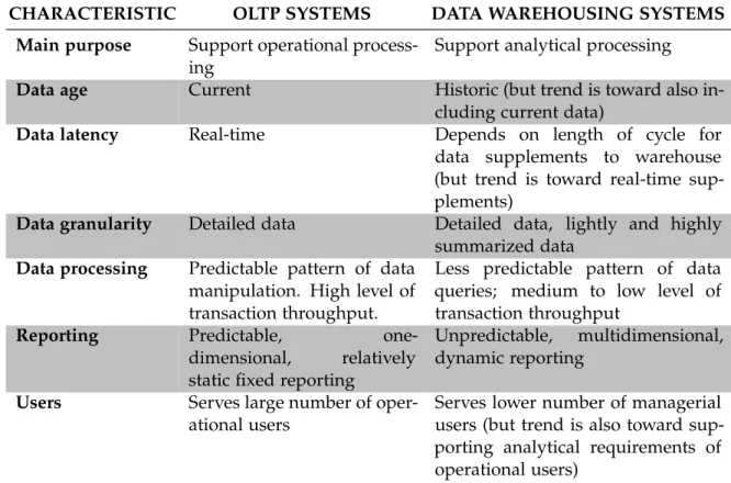
In the enterprise environment it is interesting to analyze and compare both recent and historical data to obtaining better insights on the business process. This way, data is usu-ally moved from the transactional systems to a central analytical database known as Data Warehouse (DW). This system typically encapsulates all the data of the organization. Since the only common operation in addiction to the data consulting is the refreshment of the database with data coming from theOLTPdatabases, they are considered non-volatile sys-tems. The distinction between the two presented branches of data storage is summarized in Table 5.
CHARACTERISTIC OLTP SYSTEMS DATA WAREHOUSING SYSTEMS
Main purpose Support operational process-ing
Support analytical processing
Data age Current Historic (but trend is toward also
in-cluding current data)
Data latency Real-time Depends on length of cycle for
data supplements to warehouse (but trend is toward real-time sup-plements)
Data granularity Detailed data Detailed data, lightly and highly summarized data
Data processing Predictable pattern of data manipulation. High level of transaction throughput.
Less predictable pattern of data queries; medium to low level of transaction throughput
Reporting Predictable,
one-dimensional, relatively static fixed reporting
Unpredictable, multidimensional, dynamic reporting
Users Serves large number of oper-ational users
Serves lower number of managerial users (but trend is also toward sup-porting analytical requirements of operational users)
Table 5.: OLTP vs Data Warehousing systems. Based onConnolly and Begg(2014, p. 1227)
1.3.1 Data Modeling
The complete analysis ofDWdesign and implementation methodologies is out of the scope of this dissertation. However, the interested reader can consultKimball and Ross(2011) and
1.4. Challenges & Goals 12
Inmon et al.(2002) to understand the two main distinct approaches. This document is based
on Kimball’s method.
Kimball’s business dimensional life-cycle defines a dimensional modeling phase aiming to convert data into a standard and intuitive format, where data can be more efficiently accessed (Connolly and Begg,2014, p. 1261).
Kimball defines two distinct sets of attributes: measures and dimensions. Measures should be contained in a central table (the fact table); they correspond to aggregable data, like monetary values or number of sales. Dimensions are the context that help to under-stand the meaning of those measures.
As stated, the fact table should be the central part of the database, surrounded by dimen-sion tables to form a star schema (Connolly and Begg, 2014, p. 1261). If dimension tables
are linked to other dimension tables, the schema is denoted snowflake.
The concepts presented in this section are the base of OLAP theories. However, the simple differentiation of transactional and analytical queries is enough to support the com-prehension of the conducted work. Multidimensional analysis techniques can also be used with the approach presented in Section2, but its implementation is out of the scope of this
dissertation.
1.4 c h a l l e n g e s & goals
Macedo and Oliveira (2015) proposed a way to replace RA by LA to encode and resolve
OLAP queries. Pontes(2015) tested the efficiency of such theories in a distributed
environ-ment built with the Hadoop framework (Shvachko et al., 2010). Considering the
unsatis-factory, but promising results, Oliveira and Caldas(2016) implemented a simple query in
shared memory, already outperforming PostgreSQL.
To extend the test suite from a single query to a larger, and then more solid group of queries,Ribeiro et al.(2017) worked on the implementation of multiple and more complex
queries. Meanwhile, Afonso and Fernandes (2017) provided them the LA scripts of the
tested queries, obtained when searching for a generic algorithm to convert a SQLquery to
LAequivalent.
This dissertation aims the consolidation of all previous work in a single piece of software. The main goals are the development of a DBMS based on the LA approach, as well as its validation with an industry standard benchmark suite and its performance evaluation through a comparison with standard market solutions.
The key challenges the author had to face included:
• the choice of an adequate format to represent and process very large sparse matrices; • the performance evaluation of the alternative algorithms and implementations to
1.5. Contribution 13
• the selection of a set of representative queries to validate theLAengine;
• the setup of a testbed environment with the competitive DBMS and the consequent reliable performance measurements.
1.5 c o n t r i b u t i o n
This dissertation is a follow-up of the stated projects to build a new integrated framework to aid the efficient use of aLA DBMS. To identify the key contributions is not straightforward task: the major one was certainly the proposal of a modular architecture to address queries encoded in SQL, while the other ones are mostly related to an efficient implementation of these modules. The following contributions should be outlined:
• the complete re-design of the previous kernel ofLAoperations;
• the development of a code generator that takes LAQ scripts as input and produces the equivalent C++versions;
• the validation of the code generator with several inputs from a standard benchmark suite;
• the performance tuning of the LAQ approach and a performance evaluation with standardDBMSs.
One of the key outcomes of this work is the paper ‘‘Typed Linear Algebra for Efficient Ana-lytical Querying” (Afonso et al., 2018) submitted to VLDB. The received reviews gave very
relevant clues for a further improvement of the work, which are included and discussed in the Future Work section in the last Chapter of this dissertation.
1.6 d i s s e r tat i o n o u t l i n e
Chapter 2presentsTLAand how it can be used to power a database systems and encode
relational queries. Chapter3presents the architecture and implementation details of the
de-veloped framework. Chapter4 specifies how the system was validated and benchmarked,
also comparing its performance with other systems. Finally, Chapter 5contains some
con-siderations on the developed work, as well as relevant information on how the system can be extended.
It is also noteworthy that some parts of the document were extracted from previous publications for which the author has contributed. More specifically, Chapter 2 contains
parts of a previous report byAfonso and Fernandes(2017), and Chapter4 reproduces the
analysis made for Afonso et al. (2018), which was carried in parallel with the work being
2
T Y P E D L I N E A R A L G E B R A F O R O L A P
As stated byStonebreaker et al. (2015), the “SQLStandard is both ambiguous and
underspeci-fied”. Despite all its drawbacks, SQL is undoubtedly the most used query language in the market, and the recommended interface for any new implemented system. This way, aLA
solution will be introduced as an alternative encoding for relationalSQL.
Afonso and Fernandes (2017) developed a novel attempt to define a Domain Specific
Language (DSL) to describe the LA operators, derived from SQL queries. Although the proposed solution is not full SQL compliant, it contains an objective introduction to the
TLAconcepts, forming the basis of the current analysis.
2.1 l i n e a r a l g e b r a i c e n c o d i n g o f d ata
SinceLAworks mainly with matrices, it is crucial to understand how information, initially encapsulated in relations, gets converted into matrices.
The LA encoding must be done separately for each attribute in the database, taking advantage of the columnar data access and making it possible to ignore useless attributes for each computed query.
2.1.1 Dense Vectors
The first data representation model is a straightforward extraction of an attribute from the data table. Its representation is a dense vector, as shown in (1). The ShipPriority attribute
from the Orders table will be used and, from now on, named oshippriority.
oshippriority =
1 2 3 4
h i
1 2 1 3 (1)
2.2. Type Diagrams 15
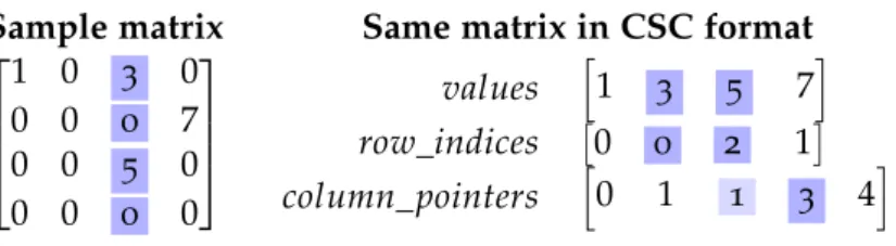
2.1.2 Sparse Matrices
With the attribute represented in a dense vector format, it is now necessary to convert it into a matrix. As seen in (2), the matrix contains the same information as the vector (1), being
a direct conversion from it. The row labels are the set of distinct values that constitute the previous vector. Obviously, repeated values only need to be represented once. The number of columns of the defined matrix matches the length of the dense vector.
oshippriority = 1 2 3 4 1 − 1 − 1-URGENT − 1 − − 2-HIGH − − − 1 3-MEDIUM (2)
Each value (“1”) in the matrix means that the record defined by the respective column number contains the value specified by the matrix row. For instance, a “1” in column “4” at the row labelled “3-MEDIUM” means that the 4th element of the array is a “3-MEDIUM”.
This conversion process creates functional matrices composed by, at most, a single value per column, that can be efficiently represented in a sparse format, as accomplished by
Ribeiro et al.(2017).
2.2 t y p e d i a g r a m s
The concept ofTDis also crucial in this approach. In (3), a diagram representing a single
matrix of width #o and height SP can be seen. It shows the type of matrix (2) that represents
the attribute oshippriority.
SP #o
oshippriority (3)
Afonso and Fernandes(2017) also used a standard notation for naming the dimensions
of the matrix. The number of records in the table is represented by the character # followed by the first letter of the tables name (in this case, the table is named Orders, hence #o).
The number of rows in the matrix is the cardinality of type SP, totalising the distinct values in the attribute oshippriority. This abbreviation comes from the combination of the first letter of each word in the attribute’s name.
It is also relevant to mention that this arrow notation is typically used to represent func-tions. In this case, it receives an argument of type #o and returns a value of type SP.
The created matrix does just that. For a given row of the data table (#o) its corresponding column in the matrix identifies its attribute value (SP), by checking the row in which the
2.3. Linear Algebra Query language 16
"1" is contained in the bitmap. This creates this notion that a matrix can be thought of as a function.
This notation can be scaled and composed to represent a full database schema. In (4) the
attributes in Tables2and3are placed in the equivalentTD.
#l OK #o OD Q SP lorderkey lquantity oorderkey oshippriority oorderdate (4)
The first thing to notice are the two tables. These are characterised in the diagram by all the attributes that compose them. Obviously, attributes of the same table have the same number of registers, hence deriving from the same point in theTD.
Another aspect introduced with this diagram are the joins between tables. In this case, the table Lineitem has an attribute (lorderkey) that is a foreign key pointing to the primary key of the table Orders.
Since null values are not allowed in OLAP databases, every single value of the foreign key attribute (lorderkey) must be present in the primary key (oorderkey).
This validates the invariant that the cardinality of the foreign key is lower or equal to the one of the primary key.
As this representation abstracts the table’s data, the bitmaps containing the foreign keys will have as many rows as the primary key, culminating in the same dimension in the diagram (OK).
Finally, note how in lquantity the attribute name was intentionally positioned over the matrix first letter. This notation was extracted from Oliveira and Macedo(2017), allowing
the differentiation between OLAPmeasures and dimensions.
2.3 l i n e a r a l g e b r a q u e r y l a n g ua g e
TheLAapproach presented by (Afonso and Fernandes,2017) not only introduced a distinct
way of encoding data, but also specified a set of operations capable of reproducing typical database queries. To formalise this set of operations in such a way that makes it suitable to be used by any developer, and capable of supporting an automatic conversion fromSQL
queries, a newDSLwas defined and namedLAQ.
This new language includes three key algebraic operators, from which all the LAQ op-erations are implemented: Dot, Khatri-Rao and Hadamard-Schur products. Three other derived operations are introduced to cover the complex syntax ofSQL: the Filter, Fold, and Lift operators.
2.3. Linear Algebra Query language 17
2.3.1 Dot Product
Mathematically, this product corresponds to the matrix multiplication, where A×B = C, being only applicable if the number of columns of the matrix A matches the number of rows of the matrix B.
It can be defined as follows: for any entry v of C in the position [x, y] (where x≤i∧y≤
k), v is calculated by summing the product of all j values in the x row of A by the j values in the column y column of B. In (5) a sample product is displayed.
1 2 3 4 5 6 . " # 1 2 3 4 5 6 = 1×1+2×4 1×2+2×5 1×3+2×6 3×1+4×4 3×2+4×5 3×3+4×6 5×1+6×4 5×2+6×5 5×3+6×6 = 9 12 15 11 26 33 29 40 51 (5)
Again, thinking of a matrix as a function, leads to the use of its specific properties. One of the most useful is the function composition. As seen in (6), the requirements for function
composition and matrix multiplication are the same, which allows a similar representation.
j k
i
M
N
M.N (6)
This property can be visualised in the TD notation. Considering the multiplication of two matrices (N and M), their composition can be represented by (M.N), thus the “dot” in the product’s name.
Another interesting aspect of this property is that the dimensions have to align, just like types in function composition. It is also very perceptible to see the result matrix dimensions in the diagram. In this case, they are (i×k).
2.3. Linear Algebra Query language 18
2.3.2 Khatri-Rao Product
The Khatri-Rao product of two matrices is represented by AOB =C. In this product, each
row of the matrix A is multiplied by the whole matrix B (row by row), and the result is stored in the final matrix C.
If the initial matrices have dimension of (i×k) and (j×k) respectively, the result matrix will have ((i∗j) ×k) dimension. In (7) its application is displayed.
" # 1 2 3 4 O 1 2 3 4 5 6 = 1×1 2×2 1×3 2×4 1×5 2×6 3×1 4×2 3×3 4×4 3×5 4×6 = 1 4 3 8 5 12 3 8 9 16 15 24 (7)
In (8) it is possible to establish a parallelism between this operator and a function split,
defined by (f Og)x = hf(x), g(x)i. One of the important properties of this operator (also
depicted in the diagram) is that no information is lost. From the result of a Khatri-Rao, one or both of the initial matrices can always be retrieved.
i i
×
j jk
π1 π2
M MON N (8)
2.3.3 Hadamard-Schur Product
The Hadamard-Schur product is defined only for matrices of the same type, i.e. matching dimensions. A×B is implemented by multiplying every element in A by the corresponding element in B and storing it in the same position on matrix C. This way, the resulting matrix matches the dimensions of the original matrices, as seen in (9).
" # 1 2 3 4 × " # 5 6 7 8 = " # 1×5 2×6 3×7 4×8 = " # 5 12 21 32 (9)
2.3. Linear Algebra Query language 19
2.3.4 Filter
The attribute filter is the equivalent operator to the relational selection, which filters the columns of a matrix based on the labels of its corresponding rows. Specifically, this operator has, as input, both a predicate and a matrix. The predicate is directly applied to the labels of the matrix, generating a boolean vector that states which labels comply with the predicate. After this, a dot product between the result vector and the initial matrix is made. This generates another boolean vector, which identifies the columns that have a row satisfying the predicate. TheTD(10) represents this clearly.
i j
1
f
M
f .M=σ(Mf) (10)
To understand this, an example is given. The matrix in (11) shows the representation of
the attribute oshippriority in a matrix format. The applied filter (12) is a predicate that selects
non-urgent shipments. oshippriority = 1 2 3 4 1 − 1 − 1-URGENT − 1 − − 2-HIGH − − − 1 3-MEDIUM (11) 6=’1-URGENT’=
1-URGENT 2-HIGH 3-MEDIUM
h i
− 1 1 (12)
The matrix in (13) is the result of the dot product of (12) by (11). It is a sparse boolean
vector that specifies whether each column in the original matrix has a row that corresponds or not to a valid predicate.
σ
(oshippriority6=’1-URGENT’) =1 2 3 4
h i
2.3. Linear Algebra Query language 20
2.3.5 Fold
A “!” is a vector of arbitrary length filled with "1"s. It is typically used to condense informa-tion, by reducing one of the matrix dimensions to the unit when both are multiplied. The
TDin (14) exemplifies this process.
i j
1
f old(M)=M.!o M
!o (14)
This way, a new vector is obtained, having as many rows as the initial matrix. Each value equals the fold of all of the elements of the corresponding row in the original matrix using the aggregation function of theSQLlanguage, for instance: sum, count, avg, min, and max. By directly applying the composition in (14), the sum and count aggregation functions
can be implemented. Furthermore, the average operator can be theoretically defined by the division sum/count. A practical implementation can be optimised to do this division in a single operation, encapsulated in the fold operator. The example in (15) illustrates the
explained operator. It is applied to obtain the sum of lquantity.
sum(lquantity) = h i 28 44 13 35 . 1 1 1 1 = 120 (15) 2.3.6 Lift
The lift operator applies a mathematical expression, defined by a lambda function, to a set of vectors, corresponding to the function arguments. This is done for each element in the provided vector(s), creating a new one with the obtained results, as exemplified in (16).
li f t(2×lquantity) =2×
h i
28 44 13 35 =
h i
2.4. Conversion algorithm 21
2.4 c o n v e r s i o n a l g o r i t h m
The current system is oriented towards analytical querying. Considering the complexity of such queries, translating a SQL query into a series of LA operations has a negligible performance overhead in the complete query run-time. Yet, there are several paths that can be taken to reach the same query output. This way, certain decisions can be made to produce the most efficient one.
Although a possible approach would be to produce a range of viable alternatives and then pick the best one based on a predicted cost, Afonso and Fernandes(2017) developed
a theoretically sustained algorithm, capable of providing an efficientLAexpression for any supportedOLAPquery.
This way, as performance is a priority, it is crucial to have a precise idea of the cost of each operation to prioritise the most efficient ones during the conversion phase. A brief study conduced by Afonso and Fernandes (2017) revealed the dot product as the most costly
operator1
, so the full development process was oriented to avoid its usage. Also, filtering an attribute results in a reduction of the number of non-zero elements in the filtered matrix. Computing these operations in the initial stages of the query processing results in a more efficient solution, thus making it another priority.
2.4.1 The approach
Afonso and Fernandes(2017) found the implementation of a generic algorithm to convert
any given SQLquery to itsLAQcounterpart a complex task.
This complexity raises from two major obstacles. The first is the high complexity ofSQL
syntax and the variety of possible queries it can describe. Another great obstacle is that
RAandLAare completely different paradigms, leading to a conversion process that does not have a direct “one to one” translation, achievable using only a Context-Free Grammar (CFG).
Like with any other complex problem, its solution is not immediately discoverable, but reached progressively. Afonso and Fernandes (2017) constantly used the queries from the
TPC-Hbenchmark to extend the algorithm’s capabilities. As more and more queries were considered, the algorithm gradually evolved to support them. The benchmark is also used in this dissertation to validate, and measure the efficiency, of the query processing.
The methodology proposed byAfonso and Fernandes (2017) is as follows:
1 Although this statement is not valid for every query, the dot product still has a negative impact in the streaming approach presented in Section3.3
2.4. Conversion algorithm 22
1) Combine independent predicates filtering the same attribute
2) Replicate the type diagram if there are disjunctions between different tables 3) Filter the attributes using the dot product
4) Combine all the filters from the same table 5) Join the tables respecting referential integrity 6) While there are more than one functional bitmap:
6.1) Compose matrices whenever possible
6.2) Khatri-Rao between all bitmaps (or Hadamard if both are vectors) 7) Merge the replicated diagrams respecting the logical tree
8) Perform the necessary operations depending on the aggregation functions 9) Sort the data as stated in the ORDER BY clause
Listing 3: SQL to LAQ convertion algorithm
1) Combine independent predicates filtering the same attribute
InRA, after the Cartesian product between all the tables involved in the query is made, the conditional expression in the WHERE clause is evaluated row by row, filtering the records.
In a columnar approach, each attribute must be evaluated separately. If the conditional expression can be divided into a set of conjunctive sub-expressions, each one only applied to a single attribute, the predicates in each set can be immediately combined, creating a new boolean vector. Otherwise, it is necessary to build the logical tree that represents the conditional expression.
2) Replicate the type diagram if there are disjunctions between different tables
If the logical tree can be fully simplified, 1) will reduce it to a single root node and this step will not change the type diagram. When this is not possible, it is necessary to replicate the type diagram.
1 WHERE l_orderkey = o_orderkey
2 AND l_orderdate = 'yesterday'
3 OR (l_orderdate = 'today' AND o_shippriority = '1-URGENT') Listing 4: Example of a SQL WHERE clause
2.4. Conversion algorithm 23
The SQL statement in Listing4 exemplifies a situation where this problem arises. The
predicates over lorderdate cannot be conjugated as stated in step 4), since it does not respect the logical expression
#l OK #o OD SP 1 1 1 lorderkey lorderdate =today =yesterday oorderkey oshippriority =URGENT (17)
The type diagram (17) represents the presented SQL code. Since this notation cannot
illustrate the difference between conjunctions and disjunctions, the logical tree in (18) was
also built.
OR
AND lorderdate =yesterday
lorderdate =today oshippriority =URGENT
(18)
The necessary conditions are now met to proceed with the replication process, creating as many new TDs as the number of ORs in the logical tree, each one of them capable of being independently solved.
#l OK #o #l OD SP OD 1 1 1 lorderkey lorderdate =today oorderkey oshippriority =URGENT lorderdate =yesterday (19)
In this particular case, since there is only one OR conditional operator, only a new type diagram is formed, splitting the conditions among the two, as shown in (19).
2.4. Conversion algorithm 24
3) Filter the attributes using the dot product
The goal is to obtain the vector that selects which columns of the bitmap will be kept, removing the others from the sparse representation. This reduces the amount of data in memory, which further improves the efficiency of the succeeding operations. Achieving this is done by composing the matrices of the filter and the attribute, as seen in (20).
#l OK #o #l
1 1 1
lorderkey ftd=f ilter(lorderdate=today)
oorderkey
f1=f ilter(oshippriority=1) fyd=f ilter(lorderdate=yesterday) (20)
4) Combine all the filters from the same table
As explained in 2), the conditions in each type diagram are independent from each other, so the diagrams can be further simplified.
At this stage, only the conditions relative to the same table can be resolved. Effectively, they can be “glued” by respecting the logical operators in the initial condition. For instance, if the initial expression was composed by an AND between two conditions, the logical conjunction would have to be performed, element by element, between the two condition vectors.
5) Join the tables respecting referential integrity
Referential integrity is a very common constraint in a relational database. This guarantees that, when a table has data that points to another table, all the made references are valid. For instance, if a given table has a foreign key that is relative to another table’s primary key, this foreign key always takes a valid value that exists in the second table’s primary key.
To guarantee this integrity, the proposed approach has to make sure that the cardinality of both attributes is the same. This may not be true if the foreign key attribute does not reference all the primary keys. Padding the foreign key’s bitmap with rows full of zeros, in all the elements that originally do not occur in it makes them both have the same cardinality, solving this problem.
2.4. Conversion algorithm 25
In theory, joining the tables can be achieved by calculating the dot product between the transpose of the primary key and the foreign key matrices, as illustrated in (21).
OK #o
#l
oorderkeyo
lorderkey join=oorderkeyo.lorderkey=ido.lorderkey=lorderkey (21)
Although this seems like a straightforward matrix composition, if the process of loading the data into the bitmaps is made correctly, the primary key of each table will always be an identity matrix, rendering the matrix multiplication redundant.
oorderkey = 1 2 3 4 5 1 − − − − 21 − 1 − − − 22 − − 1 − − 23 − − − 1 − 24 − − − − 1 25 =oorderkeyo =id (22)
The matrix in (22) contains the loaded data for the primary key of the table orders: oorderkey.
If two rows from the matrix and its respective labels were swapped, it would represent the exact same information, but it would not be the identity. Thus, this property can only be applied if the loading process is done correctly.
By employing this method, the type diagram in (23) is achieved.
#l #o #l
1 1 1
lorderkey
ftd f1 fyd (23)
6) While there are more than one functional bitmap:
The next step to complete any query is to obtain a single functional bitmap. This bitmap specifies which values of the measure(s) should be considered, ignored or aggregated. The cardinality of this bitmap matches the number of rows of the query result, which is the same as the product of the cardinalities of all attributes involved in the GROUP BY clause. Its number of columns is equivalent to the number of records in the fact table.
2.4. Conversion algorithm 26
Over this bitmap, from now on named function, all the aggregation operations can be applied. In this specific case, the translation process is being made over a simple SQL
snippet, without a GROUP BY statement, thus the obtained function is a vector.
Since the practical meaning of the data stored in intermediate matrices starts to be quite ambiguous, the final steps to achieve the query solution are less intuitive than the previous ones. In summary, the Khatri-Rao product is used to merge the attributes in the GROUP BY clause, and the dot product to filter attributes using specified predicates, as well as join tables.
6.1) Compose matrices whenever possible
By applying the dot product, the composition in (23) is simplified and the type diagram in
(24) is obtained.
#l #l
1 1 1
f1.lorderkey
ftd fyd (24)
6.2) Khatri-Rao between all bitmaps (or Hadamard if both are vectors)
Like mentioned, the Hadamard product can be used instead of the Khatri-Rao. In this case, after applying the dot product, a bifurcation was established, creating an opportunity for the usage of this rule. The type diagram (25) demonstrates the end result.
#l #l
1 1
ftd×(f1.lorderkey) fyd (25)
7) Merge the replicated diagrams respecting the logical tree
Using the logical tree calculated in 2), it is possible to join the functions of all type diagrams in a single one, using the logical disjunction element by element.
2.5. Conversion Example 27
The functional bitmap in (26), represents the fullLAtranslation of the initial WHERE
state-ment.
1 #l
f unction=fyd∨(ftd×(f1.lorderkey))
(26)
8) Perform the necessary operations depending on the aggregation functions
An aggregation function will produce a dense vector, with as many rows as the SELECT statement cardinality. The value of each element depends on the applied aggregation func-tion. These functions reduce every row of the matrix to a single value and, as explained in section2.3.5, are globally defined as the foldLAQoperator.
Knowing that both a measure vector and a functional bitmap are available, the necessary conditions are met to determine the last set of LAoperations that translate the query. The five major aggregation functions are supported (count, sum, average, min and max).
The count operation can be calculated using only the functional bitmap. This makes it so that the measure vector does not have to be loaded into memory, making it the most efficient of the aggregation functions.
Note that the count of the desired records is made by “summing” all the “1”s in the bitmap. Thus, to implement the sum operation, it is only necessary to put the measure values in the place of the “1”s before they are aggregated, using the Khatri-Rao product (or the Hadamard if the function is a vector).
Although the average is the more complex of the three operators, it can be easily obtained by dividing the result of the other ones, using the formula: average = sum/count. If the sum and/or count are not needed, it can also be incrementally calculated, storing the actual average and count.
The min and max functions follow a similar strategy, searching all the elements of an attribute for the min and max values.
9) Sort the data as stated in the ORDER BY clause
Without going through the contents of the matrices, it is impossible to perform a sort. For this reason, the content of the ORDER BY clause is directly transcribed to theLAQscript.
2.5 c o n v e r s i o n e x a m p l e
To consolidate all previous concepts and to better understand the utility of the introduced operators, aSQLquery will be translated to aLAQscript. The first step to solve any query
2.5. Conversion Example 28
is to build the correspondent TD. Using the query in Listing 1 as example, the TD that
represents it is depicted in (27).
This diagram stands as a visual representation to support the query conversion process. It does not demand any construction rules that have not been introduced in Section ??. However, the following conventions have been adopted:
• all attributes are represented as many times as they appears in theSQLscript;
• each operation to be performed removes all the input matrices from the diagram, and adds the resultant one;
• revenue represents a vector containing the result of the provided arithmetic expression applied element-wise revenue = li f t(lextendedprice∗ (1−ldiscount)), and not the filtered and aggregated values
SP OK #o CK SD #l 1 OD OD #c 1 OK 1 1 MS oshippriority oorderkey ocustkey oorderdate oorderdate lorderkey lshipdate lorderkey revenue ccustkey cmktsegment =’MACHINERY’ >’1995-03-10’ <’1995-03-10’ (27)
The first step in the query translation will be the composition of the filters. The Type Diagram in (28) illustrates the practical application of (10) to filter urgent priority records
out of the cmktsegment attribute.
MS #c
1
=’MACHINERY’
cmktsegment
2.5. Conversion Example 29
Applying this formula to all the filters in the query Type Diagram (27), results in (29),
where
σ
sd =σ
(lshipdate > ’1995-03-10’),σ
od =σ
(oorderdate < ’1995-03-10’), andσ
ms =σ
(cmarketsegment =’MACHINERY’). SP OK #o CK 1 #l 1 1 OD #c OK 1 oshippriority oorderkey ocustkey σod oorderdate lorderkey σsd lorderkey revenue ccustkey σms (29)The joins between the tables involved in the query (Lineitem, Orders, and Customers), although partially hidden, are also solvable matrix compositions.
As explained in (21), if the oorderkey attribute is transposed, it can be multiplied by lorderkey,
obtaining a single matrix as presented in (30). This matrix makes the correspondence
be-tween the records in Lineitem, as foreign keys, and the ones in Orders, as primary keys. Also, this composition is taken for free on behalf of the id property.
1 SP 1 1 #l #o #c OK 1 OD oshippriority ocustkey σod oorderdate lorderkey σsd revenue lorderkey σms (30)
2.5. Conversion Example 30
As shown in (30), there is still a composition to be made, after which the diagram (31)
can be obtained. 1 SP 1 #l #o 1 OK 1 OD oshippriority fms σod oorderdate lorderkey σsd revenue lorderkey fms ←
σ
ms.ocustkey (31)The matrices
σ
od and fms have the same dimensions, thus being combined using the Hadamard product. Many other matrices share a single dimension, for instance #l and #o, being merged with the Khatri-Rao product. The diagram containing these modifications is depicted in (32). 1 #l #o OK OD×
SP (σod×fms)OoorderdateOoshippriority σsdOlorderkey revenue lorderkey (32)Once the GROUP BY of the attributes in Orders is calculated, it can be combined with the join of the relations Orders and Lineitem, producing the diagram in (33).
1
#l OD
×
SPOK
σsdOlorderkey revenue
((σod×fms)OoorderdateOoshippriority).lorderkey