doi: 10.5540/tema.2018.019.03.0471
A Reduced Semidefinite Programming Formulation
for HA Assignment Problems in Sport Scheduling
H. J. LARA1, A.S. SIQUEIRA2and J. YUAN2
Received on December 19, 2017 / Accepted on May 08, 2018
ABSTRACT.Home-Away Assignment problems are naturally considered as quadratic programming mod-els in binary variables. For solving the problem, different formulations are studied here. First, the problem is rewritten as a quadratic programming formulation with linear constraints, and a quadratically constrained version respectively. For large scale problem, some reduced formulation are proposed by manipulating their special structure, with 1/4 of the original size. Note that the quadratic programming formulations lead to semidefinite relaxations solved approximately by semidefinite programming method. Comparison between our SDP relaxation and the MIN-RES-CUT based formulation is given. Finally some numerical experiments are given to illustrate the characteristics of each model.
Keywords: Sports scheduling, Integer quadratic programming, Semidefinite programming.
1 INTRODUCTION
Several problems in sport scheduling have been the focus of attention in the Operational Research community, such as the Home-Away assignment problem (HA-Assignment) which assigns the label home (H) or away (A) to each match of a double round robin tournament to satisfy some decision criteria (see [6] or [7]). Some of these criteria involve minimizing the total traveling dis-tance of teams, or minimizing the number of breaks [6, 16]. Models dealing with HA-Assignment problems have been proposed as linear integer programs [6, 7, 16], or as MIN-RES-CUT prob-lems [15], and others. In the last cited article, a Semidefinite Programming relaxation (SDP) for HA-assignment was proposed. With the objective of deducing more efficient SDP models, we study alternative quadratic programming formulations for the problem, which in turn leads to other SDP relaxations with better properties than that those obtained from MIN-RES-CUT. We also provide numerical experiments illustrate the performance of the solver.
*Corresponding author: Hugo Jos´e Lara – E-mail: [email protected]
1Departamento de Engenharia, Universidade Federal de Santa Catarina-Blumenau, Rua Jo˜ao Pessoa, 2750, 89036-256, Blumenau, SC, Brazil. E-mail: [email protected]
1.1 Modeling HA-assignments
In this subsection, we introduce the mathematical definition of the HA-Assignment problem, based on [15]. Here, we deal with a double round-robin tournament with a pair number (2n) of teams. In a round robin tournament each team plays every other team twice, once at home and the other away. A slot, or round, is a date where every team plays against other team. The number of slots is 2(2n−1), each team has its home and each match is held at the home of one of the two playing teams.
Atimetableis a matrixT whose rows are indexed by a set of teamsT ={1,2, . . . ,2n}, and columns are indexed by a set of slots (rounds)S={1,2, . . . ,4n−2}. Each entry of a timetable, sayτ(t,s)((t,s)∈T×S), shows the opponent of teamt in slots. A timetableT should satisfy the following conditions:
• for each teamt∈T, thet-th row ofT contains each element ofT\{t}exactly twice;
• for any(t,s)∈T×S,τ(τ(t,s),s) =t.
The first condition means that each team plays exactly twice with every other team, while the second one establishes that the team playing withτ(t,s)in slot sshould bet. In Figure 1 we show a timetable forn=2 (four teams). Generating timetables has been focus on attention of some works in sport scheduling (see [7]). It is an easy task to randomly generate timetables. If some matches are fixed in advance, the work becomes harder ([14]).
T =
2 3 2 4 3 4
1 4 1 3 4 3
4 1 4 2 1 2
3 2 3 1 2 1
Figure 1: A timetable matrix forn=2
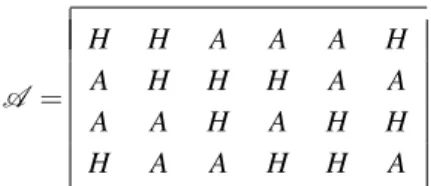
A home-away assignmentA is a matrix whose rows are indexed byT, and the columns byS respectively. Each entry of the HA-assignment,ats((t,s)∈T×S), is either ‘H’ (home) or ‘A’
(away), according to the status of teamtat rounds.
Given a timetableT, an HA assignmentA = (ats)((t,s)∈T×S)is said to beconsistentwith T if it satisfies:
C1∀(t,s)∈T×S,{ats,aτ(t,s)s}={A,H}, and
C2∀t∈T, ifτ(t,s) =τ(t,s′)ands6=s′then{ats,ats′}={A,H}.
A =
H H A A A H
A H H H A A
A A H A H H
H A A H H A
Figure 2: An HA-assignment matrix consistent withT
Our decision making is as follows: given a fixed timetableT, find a HA-assignmentA, consis-tent withT, according to some criteria. Break minimization and minimizing the total traveling distance, for instance, provides decision criteria based on a quadratic objective function in binary variables. Consequently, we propose an unified framework, grouping these decision criteria.
1.1.1 The total traveling distance minimization problem
We describe the HA-Assignment problem which minimize the total traveling distance. The distance matrixD∈R2n×2ncontain the distances between each pair of venues in the tournament.
Instance:A timetableT and distance matrixD.
Task:Find an HA-assignmentA consistent withT, minimizing the total traveling distance.
For eacht∈ {1,2, . . . ,2n}ands∈ {0,1, . . . ,4n−2}, we fixat0andat4n−1atH. The traveling
distancel(t,s)of teamtbetween roundssands+1 is defined as:
l(t,s) =
d(t,t) =0 if (at s,at s+1) = (H,H) d(τ(t,s),τ(t,s+1)) if (at s,at s+1) = (A,A) d(t,τ(t,s+1)) if (at s,at s+1) = (H,A) d(τ(t,s),t) if (at s,at s+1) = (A,H).
(1.1)
The total traveling distance for all the teams is given by
l(y) =
2n
∑
t=1 4n−2
∑
s=0 l(t,s).
1.1.2 Break minimization/maximization problems
Given an HA-assignmentA, it is said that the teamt∈T has a break at rounds∈S(s∈S\{1}) ifats−1=ats=Aorats−1=ats=H. The number of breaksb(A)in a HA-assignment is defined
as the number of breaks belonging to all teams. In practical sport scheduling, such as in [8], the number of breaks is required to be reduced.
Instance:A timetableT
Task: Find an HA-assignment that is consistent withT and minimizes/maximizes the number
1.2 SDP relaxations for HA-assignment problems
In [15] the HA-assignment problem is formulated as MIN-RES-CUT, and Goemans and Williamson approximation algorithm [9] was applied to the associated SDP relaxation. Our focus here is proposing an alternative scheme to get SDP relaxations, from a quadratic model which explore in more detail the special structure of the graph based problem.
1.3 Organization
The remainder of this article is organized as follows. In the next section we describe the opti-mization models to deal with our HA-assignment problem. First, we describe the MIN-RES-CUT formulation given in [15]. This combinatorial optimization problem induces a quadratic program in binary (1,-1) variables, which in turn leads to a SDP relaxation. In section 3 we describe an al-ternative integer quadratic program based on the same graph which conduce to MIN-RES-CUT, but with a simplified modeling strategy, which allows us to produce binary quadratic models with linear constraints, and with reduced size, when compared to MIN-RES-CUT. In section 4 we offer numerical results which compare the solver performance in each quadratic model, and also results comparing the SDP formulations. The last section is devoted to conclusion and final remarks.
2 OPTIMIZATION MODELS
In this section we describe some equivalent optimization models to treat HA-Assignment prob-lems. We first describe the MIN-RES-CUT formulation, and SDP relaxation established in [15]; then our quadratic formulations which leads to alternative SDP relaxations are proposed.
2.1 MIN RES CUT and SDP Relaxation
Suzuka, et.al. proposes in [15] a MIN-RES-CUT formulation for HA-Assignment problems minimizing the total traveling distance, and in [12] for break minimization. Their motivation was to solve the problems via SDP relaxations. We first describe the general form for the MIN-RES-CUT problem and the associated SDP relaxation.
Consider an undirected graphG= (V,E) with vertex setV and edge set E, and nonnegative weight functionw:E→R+. For any vertex subsetV′⊆V we defineδ(V′) ={{vi,vj}:vi,vj∈ V;vi6∈V′∋vj}. The MIN-RES-CUT problem is defined as follows: Given a graphG= (V,E),
a specified vertexr∈V, a weight functionw:E→R+and a setEcut⊆ {X⊂V:|X|=2}, find a vertex subsetV′as solution of the combinatorial optimization problem:
minimize ∑e∈δ(V′)∩Ew(e)
subject to r6∈V′ Ecut⊆δ(V′)
It is known that MIN-RES-CUT is a NP-hard problem (see for example [11]). The base for an SDP relaxation associated to MIN-RES-CUT is the following binary quadratic programming formulation: For eachv∈V, letxvbe a binary variable with valuexv=−1 ifv∈V′, orxv=1
if v6∈V′. Then, the first constraint is imposed byxr =1, and the second by xvxu=−1 for
{u,v} ∈Ecut. The objective function add weightwuvife={u,v} ∈δ(V′)∩E; that is ifeis an
edge and its ends are in opposite sides of the cut defined byV′. By using these binary variables, the objective function becomes 14∑u,v∈Vwuv(1−xuxv). Finally, the constraint xv∈ {−1,1} is
imposed byx2
v=1. The above considerations provide the binary quadratic model:
minimize l(x) =1
4∑u,v∈Vwuv(1−xuxv)
subject to x2v=1 ∀v∈V
xuxv=−1 ∀{u,v} ∈Ecut xr=1.
(2.2)
From this quadratic formulation, an SDP relaxation is built as follows: Form1=|E|, letW = diag(w)be them1×m1 diagonal matrix with the weightswassociated to the edges in the above problem as diagonal elements. ForC=1
4[diag(We−W)]andX, a symmetricm1×m1 matrix,
the SDP relaxation is
minimize l(X) =hC,Xi
subject to Xvv=1 ∀v∈V Xuv=−1 ∀{u,v} ∈Ecut
X0.
(2.3)
If x∈ {−1,1}m1 is a feasible solution for (2.2), thenX =xxT is feasible for (2.3). The last
problem is a relaxation because a solution for (2.3) does not necessarily provides a solution for (2.2). However, good approximated solutions for (2.2) can be extracted by Goemans and Williamson’s procedure ([9]).
2.1.1 MIN-RES-CUT formulation for HA-assignment problems
The MIN-RES-CUT formulation in [15] for the total traveling distance minimization HA-Assignment problem is described as follows: Given a timetableT = (τ(t,s))((t,s)∈T×S), consider an artificial vertexrand construct the graphG= (V,E)as:V={vts:(t,s)∈T×S}∪{r}
is the vertex set,E={{vt(s−1),vts}:t∈T,s∈S\{1}} ∪ {{r,vts}:(t,s)∈T×S}, the edges, and Ecut ={{vts,vτ(t,s)s}:(t,s)∈T×S} ∪ {{vts,vts′}:t ∈T,s,s′∈S,τ(t,s) =τ(t,s′),s6=s′} the
restriction set.
A subset of the verticesV′⊂V is feasible for the MIN-RES-CUT formulation if r∈/V′ and
Ecut ⊂δ(V′). Note that feasibility here is associated onl to the partition of the vertex set, that is
the edges of the graph only participates at the objective function.
(C1) each pair of vertices corresponding to a match is inEcut, and (C2) for each team, every pair
of vertices corresponding to matches with a common opponent is inEcut.
2.1.2 Minimizing the total traveling distance
Now, we describe the minimization of the total traveling distance: Consider the traveling distance
l(t,s), between the venues where matches in rounds s and s+1 are held, as in (1.1), and denote byt′=τ(t,s)andt′′=τ(t,s+1)the teams which plays in these rounds. Then
l(t,s) =d(t′,t′′)|vts∩V′||vts+1∩V′|+d(t,t′′)(1− |vts∩V′|)|vts+1∩V′|
+d(t′,t)|vts∩V′|(1− |vts+1∩V′|)
(2.4)
where|vts∩V′| ∈ {0,1}according tovts∈V′orvts6∈V′. The functionl(t,s)is quadratic on the
binary variables ({0,1}). These binary variables are associated with the verticesvts∈V(instead
of the edges). The idea in [15] is to model HA-assignment problems as MIN-RES-CUT. To do it, a (linear) weight function on the edges should be defined. In (2.4) there is a quadratic relation on binary variables associated to the vertices, not linear weights on the edges. To fix it, they performed the following linearization: Sincer∈/V′, we have
|vts∩V′|=|{r,vts} ∩δ(V′)|for allvts∈V.
On the other hand, taking|{vts,vts+1} ∩δ(V′)| ∈ {0,1}the product in equation (2.4) is modeled
as
|vts∩V′||vts+1∩V′| =12(|{r,vts} ∩δ(V′)|+|{r,vts+1} ∩δ(V′)|
−|{vts,vts+1} ∩δ(V′)|).
(2.5)
Merging (2.5) into (2.4) we obtain a linear function on binary variables centered at the edges, as needed. The weights of the objective function are the coefficients for |{r,vts} ∩δ(V′)|,
|{r,vts+1} ∩δ(V′)| and|{vts,vts+1} ∩δ(V′)|; and the constraintsr∈/V′ andEcut ⊂δ(V′). We
denote byW1 this set of weights.
2.1.3 Minimizing the number of breaks
There is a break between round sands+1 if (ats,ats+1)∈ {(H,H),(A,A)}. The number of
breaksb(t,s)betweensands+1 can be modeled by
b(t,s) =|vts∩V′||vts+1∩V′|+ (1− |vts∩V′|)(1− |vts+1∩V′|)
which share characteristics with (2.5), being a quadratic relation in the same binary variables. This relation leads to another coefficient matrixW2 of weights similar toW1.
2.1.4 The MIN-RES-CUT SDP relaxation
The combinatorial problem in (2.1) with the specific data provided by the graphG= (V,E), the setEcut and weight matrixW1 (orW2) specified in this section provides a combinatorial
also specified from (2.2) and (2.3) for the abovementioned data, leading to the following MRC SDP relaxation:
Minimize l(X) =hC,Xi
subject to Xvv=1 v∈V1 Xvw=−1 {v,w} ∈E1cut
X0
(2.6)
withC=1
4diag(We−W), which is the formulation given in [15].
3 ALTERNATIVE FORMULATIONS FOR HA ASSIGNMENT PROBLEMS
In this section we construct an alternative SDP relaxation for HA-assignment problems, based on quadratic programming in binary variables, which consider in more details the special structure of the assignment problem. The MIN-RES-CUT formulation described in section above also leads to a quadratic programming problem in binary variables, and consequently to a SDP relaxation. The structure of the constraints in this formulation is a consequence of the graph structure which consider each node independent of the other. Our formulation group the nodes in classes, leading to a simplification of the resulting model. The first tool that we use is described in next subsection:
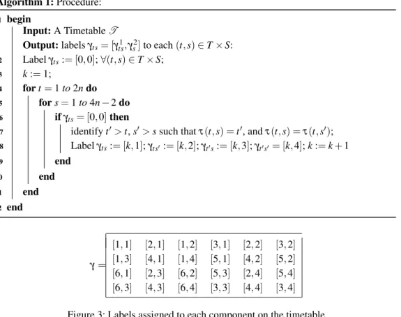
3.1 Dealing with timetables
In [13] is proposed a procedure to build a partition in a timetable, in order to extract crucial information from it, and simplify the optimization models. We here formalize such procedure. Given a timetableT and the index setT×S, we construct a partition of the indices according to the following observation: For each(t,s)∈T×S, there exist unique indices(t′,s′)∈T×S, such that the indices in the set{(t,s),(t,s′),(t′,s),(t′,s′)}are related each other, and isolated from the rest of the indices.t′=τ(t,s)is the team which plays witht in slots, ands′ is the slot where the two teams play again. Thus we can partition the index setT×SintoK=n(2n−1)subsets. Furthermore, we can order the elements in each group by appearance order in the table from left to right and from up to down. The following procedure assigns the labelγts= [γts1,γs2]to each
(t,s)∈T×S:
First let us define the setK(k) ={(t,s)∈T×S:γ1
ts=k}Clearly|K(k)|=4, because four
labelsγ1
ts=kwhere assigned in each step. The procedure pass though the timetable sequentially,
by visiting each of the(t,s)components from left to right, and form up to down. Each component ofT×Sis labeled once, placing it into theK(k)group, for somek=1, . . . ,n(2n−1). It is clear that fork16=k2,K(k1)∩K(k2) =/0, since each component is labeled once. This last observation
Algorithm 1:Procedure:
1 begin
Input:A TimetableT
Output:labelsγts= [γts1,γs2]to each(t,s)∈T×S:
2 Labelγts:= [0,0];∀(t,s)∈T×S;
3 k:=1;
4 fort=1to2ndo 5 fors=1to4n−2do 6 ifγts= [0,0]then
7 identifyt′>t,s′>ssuch thatτ(t,s) =t′, andτ(t,s) =τ(t,s′); 8 Labelγts:= [k,1];γts′:= [k,2];γt′s:= [k,3];γt′s′= [k,4];k:=k+1
9 end 10 end 11 end 12 end
γ=
[1,1] [2,1] [1,2] [3,1] [2,2] [3,2] [1,3] [4,1] [1,4] [5,1] [4,2] [5,2] [6,1] [2,3] [6,2] [5,3] [2,4] [5,4] [6,3] [4,3] [6,4] [3,3] [4,4] [3,4]
Figure 3: Labels assigned to each component on the timetable
3.1.1 Quadratic constraints by using the partition
Let us give a closer look at the constraints in (2.6). By using the partition provided byK(k),k= 1, . . . ,n(2n−1), we can characterize the restriction setE1cutas follows: We denote byE1cut(k) =
{{vtksk,vtks′k},{vtksk,vtk′sk},{vtks′k,vtk′s′k},{vtk′sk,vtk′s′k}}, and observe thatE1cut=∪
n(2n−1)
k=1 E1cut(k).
So we have an explicit formulation for the second group of constraints in the above model, namely
X(t
ksk)(tks′k)=−1
X(t
ksk)(tk′sk)=−1
X(t
ks′k)(tk′s′k)=−1
X(t′
ksk)(tk′s′k)=−1,
fork=1, . . . ,n(2n−1)(denotingX(ts)(tˆsˆ)=Xvvˆforv=vtsand ˆv=vtˆsˆ). We shall use this explicit
3.2 Alternative quadratic programming formulations for HA-assignment problems
We here propose an alternative quadratic programming formulation which in turn leads to another SDP relaxation. It will be shown that the size of this new formulation, in terms of the number of variables is 1/4 of the size of (2.2). Numerical advantages will be exhibited too.
Let us consider the graph G= (V2,E2)whose vertex set isV2={vts:(t,s)∈T×S}, and
edgesE2={{vts−1,vts}:t∈T,s∈S\{1}}, and the partitionK defined earlier. We here shall
describe the formulation for the total traveling distance minimization problem. For minimization of breaks, the development is analogous. Recall that the traveling distancel(t,s)of teamtfrom slotsto slots+1 is equivalent to (2.4) which is a quadratic function in binary{0,1}variables. The MIN-RES-CUT formulation given in [15] replaces l(t,s) by a linear function in binary variables centered at the edges, and then establishes a quadratic{1,−1}model to deal with it, through an SDP-relaxation. We here propose to employ the original quadratic objective function (2.4), which is naturally defined in binary{0,1}variables, and derive an SDP-relaxation from it. Let us denote byyts∈ {0,1}with value 0 ifvts∈/V′and 1 ifvts∈V′. The equation (2.4) becomes:
l(t,s) =d(t′,t′′)ytsyts+1+d(t,t′′)(1−yts)yts+1+d(t′,t)yts(1−yts+1)
=d(t,t′′)yts+1+d(t′,t)yts+ (d(t′,t′′)−d(t,t′′)−d(t′,t))ytsyts+1
(3.1)
fort=1, . . . ,2nands=1, . . . ,4n−3. Initial and final coefficients arel(t,0) =d(t,τ(t,1))yt1and l(t,4n−2) =d(τ(t,4n−2),t)yt4n−2respectively. The entire objective function have the form
l(y) =
2n
∑
t=1 4n−2
∑
s=0
l(t,s) =cTy+1 2y
TQy.
The quadratic formQcontains nonzero elements only on the entries above and below the diag-onal, since only two consecutive variablessands+1 are involved in the quadratic terms. Note that this formulation does not increases with the artificial vertexr.
To define the constraints we shall denote the variablesytsaccording to the partitionK of the
in-dex set. Each entry(t,s)∈T×Sis labeled withγts= [k,j],k∈ {1, . . . ,n(2n−1)},j∈ {1,2,3,4}.
Let us denoteytsbyytkskifγts= [k,1];yts=ytks′k ifγts= [k,2],yts=ytk′sk ifγts= [k,3]and finally
yts=ytk′sk′ ifγts= [k,4]. By using the{0,1}to{−1.1}transformation, namelyx(y) =2y−1 we
write the cut constraints as
(2ytksk−1)(2ytks′k−1) =−1
(2ytksk−1)(2ytk′sk−1) =−1
(2yt
ks′k−1)(2ytk′s′k−1) =−1
(2yt′
ksk−1)(2ytk′s′k−1) =−1,
fork=1, . . . ,n(2n−1), which provide the quadratic constraints
ytksk+ytks′k−2ytkskytks′k=1
ytksk+ytk′sk−2ytkskyt′ksk=1
yt
ks′k+ytk′s′k−2ytks′kyt′ks′k=1
yt′
fork=1, . . . ,n(2n−1). The result is a group of 4n(2n−1)quadratic constraints ony, which we denote for eachkand jby
1+cTk jy+1 2y
TH
k jy=0,for j=1,2,3,4.
Now we cast the problem as
minimize l(y) =a+cTy+1 2y
TQy
subject to 1+cTk jy+21yTHk jy=0,
k=1, . . . ,n(2n−1);
j=1,2,3,4.
The matrices Hk j are highly sparse, because they involve only two consecutive variables,
andQ is a tridiagonal matrix with zero diagonal. By using the relation a+cTy+1 2y
TQy=
h a
1 2cT 1 2c
1 2Q
!
, 1 y
T
y yyT
!
i, and similarly for the constraints, we write equivalently the
quadratic program as
minimize l(y) =h a
1 2c T 1 2c 1 2Q !
, 1 y
T
y yyT
!
i
subject to h 1
1 2c
T k j 1
2ck j 1 2Hk j
!
, 1 y
T
y yyT
!
i=0, k=1, . . . ,n(2n−1);
j=1,2,3,4.
y∈ {0,1}2n(4n−2).
(3.2)
To build a SDP relaxation, we replace the rank one matrix variable 1 y
T
y yyT
!
by Y ∈
R2n(2n−1)×2n(2n−1), satisfyingY0, andY
(ts)(ts)−Y(11)(ts)=0 for all(t,s)∈T×S.
The quadratic programming formulation provided by the MIN-RES-CUT model in [15] asso-ciates to each vertice of the underlying graph a binary{1,−1}variable; and the objective func-tion is defined as the sum of the linear weights on the edges (see (2.1)). In order to offer these linear weights, a linearization given by (2.5) was performed. Our proposal recognizes the orig-inal quadratic structure of the objective function (prior to be linearized) to define directly an equivalent quadratic model suitable to be relaxed through the following SDP model:
minimize l(y) =h a
1 2c T 1 2c 1 2Q !
,Yi
subject to h 1
1 2cTk j 1
2ck j 1 2Hk j
!
,Yi=0, k=1, . . . ,n(2n−1);
j=1,2,3,4.
Y(ts)(ts)−Y(11)(ts)=0, ∀(t,s)∈T×S Y 0.
3.2.1 A linearly constrained quadratic model
We can use linear constraints to model theC1−C2 conditions:
ytksk+ytk′sk=1
ytksk+ytks′k=1
−ytksk+yt′ksk=0
(3.4)
At each groupk, the first equation means that only one of the teams plays at home in slotsk.
The second equation establishes that teamtkshould play alternatively at home and away in slots sk ands′k; and the third one ensures that if the first team plays at home (away) at the first slot,
then the second team should be home (away) in the second match between them. Putting all the constraints together fork=1, . . . ,n(2n−1), we can write the above constraints as a linear system of equations, sayAy=b. Our quadratic binary program with linear constraints becomes
Minimize l(y) =cTy+1 2y
TQy
subject to Ay=b
y∈ {0,1}4n(2n−1)
(3.5)
Ais an 3n(2n−1)×4n(2n−1)matrix with entries in{0,1}, whileHis tridiagonal (with zero diagonal) 4n(2n−1)×4n(2n−1). We can directly construct an SDP relaxation from (3.5), but the special structure presented by these linear constraints allows us another simplification: By equations (3.4) we have that
yt′ ksk ytks′k yt′
ks′k
=
1 1 0
−
1 1 −1
ytksk=bk−Atkskytksk.
Denoting byzk=ytksk we write all the variablesyin function of z∈ {0,1}
n(2n−1). For eachk,
consider the subsetsBk={(tk,s′k),(tk′,sk),(tk′,s′k)}andNk={(tk,sk)}of the indicesT×S; and
constructB=∪nk(=2n−11 )BkandN=∪nk=(2n−11 )Nk. This leads us toyB=b−ANz, andyN=zwhich
in turn defines the linear transformationY byY(z) =y. The objective functionl(y)becomes
¯
l(z) =l(Y(z)) =a¯+c¯Tz+zTQz¯ ,
where ¯a=a+cTBb+bTHBBb; ¯c= (c−ATNcB−2ATNQBBb−2QNBb)T and ¯H= [ATNQBBAN+ ATNQBN+QNBAN]. Our equivalent reduced model is:
Minimize l¯(z) =a¯+c¯Tz+1 2z
TQz¯
subject to z∈ {0,1}n(2n−1), (3.6)
some metaheuristics, like genetic algorithms, without the care of generating feasible solution populations. The resulting SDP relaxation is
minimize l(Z) =hC¯,Zi subject to diag(Z) =e
Z0
(3.7)
where ¯C= a¯
1 2c¯
T
1 2c¯
1 2Q¯
!
which we call reduced SDP.
3.2.2 Comparison between the SDP formulations
Notice that the combinatorial problem (2.1) is centered at the edges of the underlying graph, in the sense that the weights in the objective function act over the edges in the feasible cut, and the constraints determine where the cut edges are chosen. When specialized to HA-assignment problems, the original formulation of the objective function, based on (1.1), in the case of total traveling distance minimization, shows a quadratic relation in binary variables defined on the vertices (not on the edges). The authors in [15] adapt the model by adding an artificial vertexr, and 2n(4n−2)additional edges (linkingrto every other vertex). The relation (3.1) provides a linearization of the objective function. Now the variables are centered at the edges, instead of the vertices, and a linear relation is obtained, as required by the MIN-RES-CUT format.
On the other hand, when the quadratic program (2.2) is formulated, binary variables (centered at the vertices) model the combinatorial problem (2.1). Simple quadratic constraints are natural to model the cut constraints, and the objective function becomes a quadratic function on these binary variables. This quadratic function is then linearized, with variables centered at the edges, to be in the sequel modeled as a quadratic program in binary variables. The number of variables is equal to the number of vertices, namely 2n(4n−2) +1.
4 NUMERICAL RESULTS
In this section we offer some computational experiments to compare the different studied models. At first, we deal with integer quadratic models, comparing the full sized and reduced versions, in a preliminary experiment, in part published at [10]. A more robust experiment is reported at the second part, comparing SDP relaxations for the HA-Assignment problem.
4.1 Integer quadratic programming models
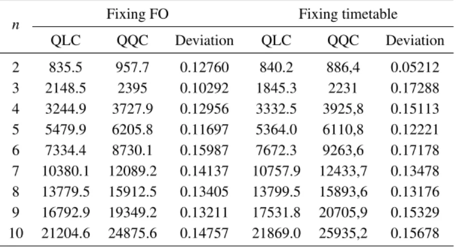
Table 1: Objective function values for quadratic and linear models with linear constraints, with full and reduced size, vs quadratically constrained quadratic models.
n Fixing FO Fixing timetable
QLC QQC Deviation QLC QQC Deviation
2 835.5 957.7 0.12760 840.2 886,4 0.05212
3 2148.5 2395 0.10292 1845.3 2231 0.17288
4 3244.9 3727.9 0.12956 3332.5 3925,8 0.15113
5 5479.9 6205.8 0.11697 5364.0 6110,8 0.12221
6 7334.4 8730.1 0.15987 7672.3 9263,6 0.17178
7 10380.1 12089.2 0.14137 10757.9 12433,7 0.13478 8 13779.5 15912.5 0.13405 13799.5 15893,6 0.13176 9 16792.9 19349.2 0.13211 17531.8 20705,9 0.15329 10 21204.6 24875.6 0.14757 21869.0 25935,2 0.15678
Three different integer programming formulations for the same problem are solved with simu-lated data: A quadratic program with linear constraints QLC (3.5), a reduced quadratic program QR (3.6), and a quadratically constrained quadratic program QQC (3.2). All computations were performed on a PC Intel(R) core(TM) i7-3632 QM, 2.20 GHZ, 64 bits.
In the first experiment, we fix the objective function and solve instances with 10 different ran-domly generated timetables, for each problem sizen, with the objective of exploring the perfor-mance of the solver in a variety of configurations (timetables). Even sharing the same objective function for each n, we solve 10 distinct instances, because different timetables lead to differ-ent constraints. For the second experimdiffer-ent we fix a timetable, and then we solve the problem for 10 different objective functions data, for each problem size (single configuration). We solve HA-assignment problems for a even number of teams, between 4 and 20. Since our objective is to compare the formulations for the problem, we use a non commercial solver which deal with both, linear and quadratic integer programs, namely SCIP [3].
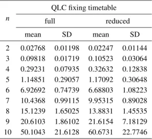
Table 2: Runtime for the quadratic models, with linear constraints, fixing the timetable.
n
QLC fixing timetable
full reduced
mean SD mean SD
2 0.02768 0.01198 0.02247 0.01144 3 0.09818 0.01719 0.10523 0.03064 4 0.29231 0.07935 0.32632 0.12838 5 1.14851 0.29057 1.17092 0.30648 6 6.92692 0.74739 6.68803 1.08223 7 10.4368 0.99115 9.95315 0.89028 8 15.1239 1.65025 13.8831 1.45535 9 20.6103 1.86102 21.6154 7.18129 10 50.1043 21.6128 60.6731 22.7746
Table 3: Runtime for the quadratic models with linear constraints, fixing the objective function.
n
QLC fixing OF
full reduced
mean SD mean SD
2 0.01881 0.00349 0.02049 0.00817 3 0.10556 0.03898 0.09833 0.02711 4 0.22068 0.06098 0.24719 0.07874 5 1.02054 0.30153 1.15223 0.54655 6 6.27446 1.73542 6.07395 1.71097 7 10.9502 1.57499 9.91357 0.59958 8 14.5375 1.38106 13.5211 1.30986 9 21.3364 1.86914 21.9286 6.80267 10 60.8347 19.6424 41.4042 22.7594
sixth columns are for the model with quadratic constraints (QQC). The remaining columns con-tain relative deviations of the values. The difference between linear constrained and quadratic constrained models is possibly because the solver only guarantee locally optimal solutions in problems with quadratic constraints.
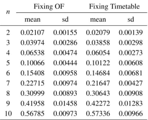
Table 4: Runtime for the quadratically constrained model (QQC), fixing the objective function and the timetable.
n Fixing OF Fixing Timetable
mean sd mean sd
2 0.02107 0.00155 0.02079 0.00139 3 0.03974 0.00286 0.03858 0.00298 4 0.06538 0.00474 0.06054 0.00273 5 0.10066 0.00444 0.10122 0.00608 6 0.15408 0.00958 0.14684 0.00681 7 0.22715 0.00974 0.21647 0.00427 8 0.30999 0.00893 0.30643 0.00908 9 0.41958 0.01458 0.42272 0.01283 10 0.56785 0.00973 0.57336 0.00966
It was expected that the running times for the reduced version in the quadratic models to be consistently smaller, but this does not occur.
Now we shall study Table 3, which provides runtime for our integer quadratic and linear pro-grams, with full and reduced size configurations, but fixing the structure (fixing a timetable). In each case we solve for 10 different objective function’s data, for each problem size. There is no clear evidence of advantage in choosing the reduced version. Sometimes is faster and in other times slower.
The Table 4 deal with runtime for both experiments, but for the quadratically constrained model (QQC). When compared with Table 2 and Table 3, we observe a huge difference in the performance. The price we pay is that global optimization is not guaranteed.
4.2 SDP models
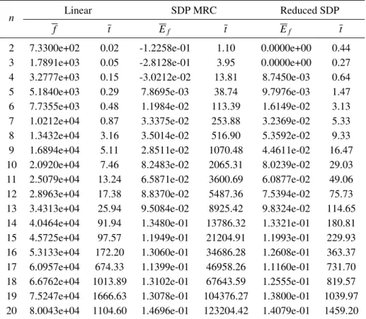
Table 5: Running times for S.
n Linear SDP MRC Reduced SDP
f t Ef t Ef t
2 7.3300e+02 0.02 -1.2258e-01 1.10 0.0000e+00 0.44
3 1.7891e+03 0.05 -2.8128e-01 3.95 0.0000e+00 0.27
4 3.2777e+03 0.15 -3.0212e-02 13.81 8.7450e-03 0.64
5 5.1840e+03 0.29 7.8695e-03 38.74 9.7976e-03 1.47
6 7.7355e+03 0.48 1.1984e-02 113.39 1.6149e-02 3.13
7 1.0212e+04 0.87 3.3375e-02 253.88 3.2369e-02 5.33
8 1.3432e+04 3.16 3.5014e-02 516.90 5.3592e-02 9.33
9 1.6894e+04 5.11 2.8511e-02 1070.48 4.4611e-02 16.47
10 2.0920e+04 7.46 8.2483e-02 2065.31 8.0239e-02 29.03
11 2.5079e+04 13.24 6.5871e-02 3600.69 6.0877e-02 49.06
12 2.8963e+04 17.38 8.8370e-02 5487.36 7.5394e-02 75.73
13 3.4313e+04 25.94 9.5084e-02 8925.42 9.8324e-02 114.65 14 4.0464e+04 91.94 1.3480e-01 13786.32 1.3321e-01 180.81 15 4.5725e+04 97.57 1.1949e-01 21204.91 1.1993e-01 229.93 16 5.3133e+04 172.20 1.3060e-01 34686.28 1.2608e-01 363.37 17 6.0957e+04 674.33 1.1399e-01 46958.26 1.1160e-01 731.70 18 6.6762e+04 1013.89 1.3102e-01 67643.59 1.2555e-01 819.57 19 7.5247e+04 1666.63 1.3078e-01 104376.27 1.3800e-01 1039.97 20 8.0043e+04 1104.60 1.4696e-01 123204.42 1.4079e-01 1459.20
5 CONCLUSIONS
In this article we study integer quadratic programming formulations for HA-Assignment prob-lems which appear in sport scheduling, and their associated semidefinite positive (SDP) relax-ations. We start from the combinatorial optimization model (2.1) given by the MIN-RES-CUT model, and previously studied in ([15]), obtaining a quadratic programming formulation based on (2.2) and it respective SDP relaxation (2.3); with de data associated to HA-assignment problems.
By exploring the special structure of the HA-assignment problem, through the modeling tools shown in the subsection 3.1, we write the integer quadratic model (3.2) which lead to the SDP relaxation (3.3), sharing the same problem size that MRC.
The quadratic model with quadratic constraints given by (3.2) behaves much better than the linear constrained one (3.5), as exhibited by Table 4. Nevertheless, the solutions are not globally optimal (see Table 1). This observation suggests that quadratic relations provide better characteristics to the solver´s performance than the linear counterparts
The main contribution of this paper are the SDP relaxations given by (3.3) and the reduced version (3.7), which is compared to the MRC relaxation introduced in [15]. In the Table 5 are shown results for instances from 4 to 40 teams. The quality of these solutions, measured by the relative errors are similar for both of the models, but for our reduced SDP relaxation the running times are much better.
ACKNOWLEDGMENTS
This work is supported in part by the Brazilian Government, through the Excellence Fellowship Program CAPES/IMPA of the first author while visiting the department of Mathematics at UFPR, Curitiba, Brazil.
RESUMO. Os problemas de alocac¸˜ao local visitante s˜ao considerados de forma natural como modelos de programac¸˜ao quadr´atica em vari´aveis bin´arias. Para resolver ditos prob-lemas, estudamos aqui diferentes formulac¸˜oes. Primeiro, o problema ´e reformulado como um programa quadr´atico com restric¸˜oes lineares, e restric¸˜oes quadr´aticas, respectivamente. Para problemas de grande porte, propomos uma formulac¸˜ao de tamanho reduzido, obtida manipulando sua estrutura especial a 1/4 do problema original. Notemos que a formulac¸˜ao de programac¸˜ao quadr´atica nos leva a uma relaxac¸˜ao semidefinida, que ´e resolvida de forma aproximada por m´etodos de programac¸˜ao semidefinida. Comparamos nossa formulac¸˜ao re-duzida de programac¸˜ao semidefinida, com a conhecida formulac¸˜ao MIN-RES-CUT. Fi-nalmente, oferecemos experimentac¸˜ao num´erica para ilustrar as caracter´ısticas de cada modelo.
Palavras-chave: Calend´arios esportivos, programac¸˜ao quadr´atica inteira, programac¸˜ao semidefinida.
REFERENCES
[1] “Introducing the MOSEK Optimization Suite 8.1.0.47” (2018 (accessed February 10, 2018)). URL https://www.mosek.com/documentation/.
[2] “CPLEX Optimization” (2018 (accessed February 3, 2018)). URL https://www.ibm.com/ analytics/data-science/prescriptive-analytics/cplex-optimizer.
[3] T. Achterberg. “Solving constraints integer programs”, volume 1 (1) (2009), pp. 1–41.
[5] I. Dunning, J. Huchette & M. Lubin. JuMP: A Modeling Language for Mathematical Optimization.
SIAM Review,59(2) (2017), 295–320. doi:10.1137/15M1020575.
[6] K. Easton, G. Nemhauser & M. Trick. The traveling tournament problem: description and benchmarks. In T. Walsh (editor), “Principles and Practice of Constraint Programming, Volume 2239 of Lecture Notes in Computer Science”. Springer, Berlin (2001).
[7] K. Easton, G. Nemhauser & M. Trick. Solving the travelling tournament problem: a combined inte-ger programming and constraint programming approach. In J.Y.T. Leung & J.H. Anderson (editors), “In Handbook of Scheduling: Algorithms, Models and Performance Analysis”. Chapman and Hall (2004).
[8] M. Elf, M. Junger & G. Rinaldi. Minimizing breaks by maximizing cuts.Operations Research Letters, 31(2003), 343–349.
[9] M.X. Goemans & D.P. Williamson. Improved approximation algorithms for maximum cut and satisfiability problems using semidefinite programming.Journal of the ACM,41(1995), 1115–1145.
[10] H. Lara Urdaneta, J. Yuan & A. Siqueira. Alternative linear and quadratic programming formula-tions for HA-Assignment problems. In “Proceeding Series of the Brazilian Society of Applied and Computational Mathematics”. SBMAC, S˜ao Jose dos Campos, SP. (2018), pp. 1–8.
[11] M. Laurent & F. Rendl. Semidefinite Programming and Integer Programming. Austria, 2002., KUniversit¨at Klagenfurt, Institut f¨ur Mathematik (2002).
[12] R. Miyashiro & T. Matsui. Semidefinite programming based approaches to the break minimization problem.Computers and Operations Research,33(2006), 1975 – 1982.
[13] J. Perdomo & H. Lara. A combinatorial optimization formulation for the HA-Assignment problem.
Publicaciones en Ciencias y Tecnolog´ıa,7(2) (2013), 127–141.
[14] C. Ribeiro. Sport Scheduling: a tutorial on fundamental problems and applications. Technical report, Department of Computer Science, Universidade Federal Fluminense, Brazil (2010). URLhttp:// www.ic.uff.br/~celso/artigas/sport-scheduling.
[15] A. Suzuka, R. Miyashiro, A. Yoshise & T. Matsui. Semidefinite Programming Based Approaches to Home-Away Assignment Problems in Sports Scheduling. Mathematical engineering technical reports, Department of Mathematical Informatics, The University of Tokyo. Japan. (2005). URLhttp:// www.i.u-tokyo.ac.jp/mi/mi-e.htm.