Intelligent modelling of temperature propagation induced by therapeutic ultrasound

INTELLIGENT MODELLING OF

TEMPERATURE PROPAGATION

INDUCED BY THERAPEUTIC

ULTRASOUND

Mestrado Integrado em Engenharia Electr´onica e Telecomunica¸c˜oes

Trabalho efectuado sob a orienta¸c˜ao de:

Prof. Dra. Maria Gra¸ca Ruano

I, Raul Manuel Ribeiro Ferreira, declare that this thesis titled, ’Intelligent modeling of temperature propagation induced by therapeutic ultrasound’ and the work presented in it are my own. Authors and works consulted during the realization of this work are properly cited and included in the reference listing.

Signed:

Date:

i

Abstract

This thesis intended to study the feasibility in applying an innovative approach to esti-mate the temperature propagation during thermal therapies, in a non invasive way. The standard reference in this field is imposed by the temperature resolution obtained with MRI techniques, 0.5oC/cm3. It was proposed to estimate the temperature evolution us-ing predictive models usus-ing b-splines neural networks evolved by the ASMOD algorithm.

Initially the data used to construct the models was characterized to provide the reader the possibility to assess if the data is trustworthy and representative of the physical phenomena intended to model. The modelling environment complexity was gradually increased which resulted in three different models typologies: SPSI, MPSI, MPMI. For each one of the different typologies the relevant features to be taken as input variables were defined along with the network structures associated with the typology.

Ensembles of neural networks were also studied in an attempt to enhance the prediction accuracy of the system. Three methods were assessed: Simple average (SA), where the average of the individual predictions is taken as the final prediction. An evolutionary strategy (ES) was also applied. Again the average of the individual predictions is taken as the final input however each individual network Ni is affected by a weight ωi. The

weight vector ω was evolved by using a evolutionary strategy. A different combination mechanism was proposed in this thesis, neural dynamic ensemble optimization (NDEO), which introduces a second layer formed by a b-spline network takes all the individual predictions as inputs, o1. . . oN where N is the ensemble size and generates an output

of, which is taken as the final prediction.

A clear division was made between the heating and cooling dynamics involved in a typ-ical thermal therapy. This division resulted in the creation of two distinct models that model the two different dynamics observed. Two experiments were always considered regarding the data used for training, validation and testing: a) Uncorrupted data. This data set is composed of the original data collected in the conditions exposed in this work; b) Corrupted data. After a contamination process, where Gaussian noise was added to the original set, the corrupted data was used to train and validate the models.

Using corrupted data to train and validate the models provides two different analysis perspectives. For one side the robustness of the system was assessed and it helps the designer to ascertain if the structure modelling power is in adequate level for the task. This last assessment is possible by observing the model behaviour in the test set. Ideally the model should only learn the dynamics of the phenomena intended to model and filter all external dynamics derived from the various possible noise sources. On the other side it alleviates the need for acquiring high quality data, which can only be captured using an invasive technique. A reliable temperature estimation method can be used to collect all the data needed to create models of complex environments.

Several models were developed for estimating the temperature curves in a non invasive way. We found that the modeling approach applied was capable of providing highly accurate predictive models. This observation holds in the experiments using Gaussian contaminated data, which evidences the robustness of the approach. A second crucial observation is that the performance figures obtained remain comparable when the mod-eling environment complexity is increased, suggesting a modelling approach with the desirable scalability.

The performance figures were obtained using relatively simple models, which might be crucial for applications with scarce resources or that require real time responses. It was observed the average model complexity evolved at a slow pace with the modelling environment complexity, which means the system complexity can be managed as the environment approaches ideal conditions.

Combining BSNNs by forming neural network ensembles creates a potential perfor-mance enhancement mechanism, if the designing is appropriated. However we noted that a great deal of effort by the designer is needed to create the favorable conditions on which combining individual forecasting entities might pay off.

When compared to the state of art, the BSNN structures over-perform the maximum absolute error obtained using MRI, which is a very impressive result. Obviously the en-vironments on which MRI operates are far more complex than the ones studied in this work. However we observed a modelling approach with very good indicators concern-ing scalability in response to increases in the complexity of the modelconcern-ing environment. Together with neural network ensemble methods the systems can be forced to be more accurate and robust. We conclude that the approach followed in this thesis is feasible, and future research is highly recommended.

Resumo

Este tese pretende estudar a possibilidade de aplicar um uma abordagem inovativa para estimar a propaga¸c˜ao de temperatura em tecidos durante termoterapias, num paradigma n˜ao invasivo. A referˆencia do estado da arte ´e imposta pela uso de t´ecnicas de ressonˆancia magn´etica (MRI), onde s˜ao obtidas resolu¸c˜oes de temperatura com erros absolutos in-feriores a 0.5 oC/cm3. Prop˜oe-se estimar a evolu¸c˜ao da temperatura atrav´es do uso de modelos preditivos, baseados em redes neuronais b-spline, evolu´ıdas pelo algoritmo ASMOD.

Inicialmente os dados utilizados foram caracterizados de forma a que o leitor possa avaliar se os dados em quest˜ao s˜ao representativos e adequados do fen´omeno f´ısico que se pretende modelar. Gradualmente a complexidade do ambiente visado na modela¸c˜ao foi aumentada, resultando em trˆes diferentes tipologias de modelo: SPSI, MPSI e MPMI. Para cada uma das tipologias as vari´aveis de interesse foram indentificadas bem como as estruturas de rede mais adequadas para o tipologia em quest˜ao.

Conjuntos combinados de redes neuronais foram tamb´em alvo de estudo numa tentativa de melhorar a efic´acia nas predi¸c˜oes dos modelos. Trˆes m´etodos foram alvo de estudo: M´edia simples (SA), onde trivialmente a m´edia do conjunto ´e tida como a predi¸c˜ao final. Uma estrat´egia evolutiva (ES) foi tamb´em considerada, resultando assim numa m´edia ponderada onde cada predi¸c˜ao individual de cada rede neuronal Nivem afectadad de um

peso ωi. Um terceiro mecanismo foi proposto nesta tese, neural dynamics ensemble

optimization (NDEO), que introduz uma segunda camada activa na arquitectura do sistema. Esta ´e constitu´ıda por uma rede neuronal que recebe como entrada todas as predi¸c˜oes individuais yi, combinando-as de uma forma activa para uma solu¸c˜ao final.

A metodologia de modela¸c˜ao preveu uma separa¸c˜ao clara entre a fase de aquecimento e arrefecimento, devido ao distanciamento existente entre a correspondente dinˆamica de subida e descida. Esta divis˜ao resultou na cria¸c˜ao de pares de modelos, referentes `as duas distintas fases da terapia. Duas experiˆencias foram sempre consideradas: a) Dados n˜ao contaminados. Este conjunto de dados corresponde ao original, n˜ao modificado e cujas condi¸c˜oes de captura est˜ao expostas neste trabalho. b) Dados contaminados. O conjunto original ´e contaminado por um processo aditivo Gaussiano. Este conjunto cor-rupto ´e usado para treino, valida¸c˜ao e teste. O uso de conjuntos de dados contaminado vem afectado de duas motiva¸c˜oes. por um lado fornece um claro teste `a robustez do

sistema e ajuda o designer a averiguar se a estrutura possui o potencial adequado ao problema. Por outro lado alivia a necessidade de recolha de dados de alta qualidade, que apenas poder˜ao ser recolhidos utilizando procedimentos invasivo.

V´arios modelos foram desenvolvidos para estimar as curvas de temperatura de uma forma n˜ao invasiva. Observou-se que a metodolgia aplicada foi capaz de construir modelos predictivos de alta exactid˜ao.

Declaration of Authorship i

Abstract ii

Resumo iii

Contents vi

List of Figures ix

List of Tables xviii

Abbreviations xxii 1 Introduction 1 1.1 Motivation . . . 1 1.2 Proposed goals . . . 2 1.3 Thesis outline . . . 3 1.4 Publications . . . 4 2 Background theory 5 2.1 Introduction . . . 5 2.2 Prediction . . . 6 2.3 Representations of curves . . . 8 2.3.1 B-Splines . . . 9

2.3.2 Approximating functions with B-splines . . . 21

2.4 Process control . . . 22

2.4.1 Modeling the temperature propagation . . . 23

2.4.2 Neural Networks . . . 25

2.4.2.1 Associative Memory Networks . . . 26

2.4.2.2 B-splines neural networks . . . 29

2.4.2.3 BSNN internal structure . . . 32

2.5 Model performance evaluation . . . 35

2.6 Model validation and stopping the training . . . 36

2.7 Enhancing forecasting . . . 38

2.8 Combining forecasts . . . 39

2.8.1 Theory behind neural networks ensembles . . . 41

2.8.2 Designing the ensemble . . . 43

2.8.2.1 Evolving the ensemble . . . 45

2.8.2.2 Increasing the ambiguity . . . 47

2.8.2.3 An ensemble of degraded networks . . . 48

2.8.3 Neural dynamic ensemble optimization (NDEO) . . . 51

3 Experimental set-up and data acquisition 54 3.1 Introduction . . . 54 3.2 Materials . . . 55 3.3 Experiment configurations . . . 56 3.4 Setting-up . . . 57 3.5 Sensor positioning . . . 58 3.6 Experimental procedures . . . 59 3.7 Experimental results . . . 60 3.7.1 Final remarks . . . 61

4 Applied estimation models 63 4.1 Introduction . . . 63

4.2 Modelling methodology . . . 64

4.2.1 Data preparation . . . 64

4.2.2 Model validation . . . 69

4.2.3 Network designs, structure selection and algorithms . . . 71

4.2.4 Adapting the free parameters . . . 74

4.3 Estimation models . . . 74

4.3.1 Network design structures . . . 75

4.3.1.1 Single-point, single-intensity (SPSI) . . . 76

4.3.1.2 Single-point, multi-intensity (SPMI) . . . 78

4.3.1.3 Multi-point, multi-intensity (MPMI) (1D) . . . 79

4.3.2 Adding noise . . . 82

4.4 Modelling approaches . . . 86

4.4.1 Keep-the-best (KTB) . . . 87

4.4.2 Simple average ensemble . . . 88

4.4.3 Ensemble optimized (ES) . . . 89

4.4.4 Neural dynamic ensemble optimization (NDEO) . . . 91

5 Results and discussion 93 5.1 Introduction . . . 93

5.2 Single-point single-intensity (SPSI) . . . 95

5.2.0.1 Results discussion . . . 105

5.3 Single-point multi-intensity (SPMI) . . . 106

5.3.0.2 Results discussion . . . 112

5.4 Multi-point multi-intensity (MPMI) 1 − D . . . 113

5.4.0.3 Results discussion . . . 123

6 Final discussion and future work 126 6.1 Introduction . . . 126

6.2 Global assessment of the performance criteria . . . 127

6.2.1 Mean Square Error . . . 127

6.2.2 Linear Weight Norm . . . 129

6.2.4 Ensembles methods . . . 132

6.3 Concluding remarks . . . 136

6.4 Reflections about the solution derived and AI . . . 138

6.5 Future research . . . 139

A B-splines under the light of the convolution operation. 142

B Data division concerning MPMI model typology. 145

C Extended results obtained with respect to SPSI typology models. 148 D Extended results obtained with respect to SPMI typology models. 189 E Results for MPMI model typology, prediction horizon h = 7 seconds. 202

2.1 One step ahead estimation, based on T past values of the process. Adapted

from [1]. . . 7

2.2 Piecing polynomials. [2] . . . 10

2.3 Three BS or order 3. Notice the three non zero Bi,3 over the interval [tj, . . . , tj+k). Adapted from [2] . . . 12

2.4 BS of order 2 with (a) simple knots, (b) a double knot. Adapted from [2] 13 2.5 B-spline of order 4 with knot sequence t = [0 1.5 2.3 4 5]. Each interval, with the respective color, represents one piece of the basis function. Figure generated with MATLAB, using the Curve Fitting Toolbox [3] . . . 15

2.6 A 6th order B-spline and the six 5th order polynomials whose selected pieces make up the B-spline. Knot sequence t = [0 1 2 3 4 5 6]. Each piece of the basis function is represented in a different color. Figure generated with MATLAB, using the Curve Fitting Toolbox [3] . . . 16

2.7 Spline function of order 3, constructed by linearly combining three B-splines of order 3. The blue lines indicate the position of knot, the gray dashed lines represent the B-splines, and the solid black line shows the resulting spline function. Control points employed a = [4 0.3 2.3]. Figure generated with MATLAB, using the Curve Fitting Toolbox [3] . . . 16

2.8 Spline function of order 3 resulting from changing the control vector. The blue lines indicate the position of knot, the gray dashed lines represent the B-splines, and the solid black line shows the resulting spline function. Figure generated with MATLAB, using the Curve Fitting Toolbox [3] . . 17

2.9 Triangular array used for evaluating k BSs of order k. [4] . . . 18

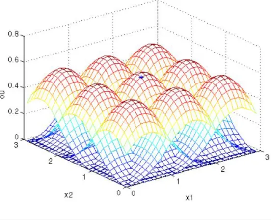
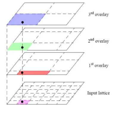
2.10 Two-dimensional multivariable basis functions formed with order 3 uni-variate basis functions. Adapted from [4]. . . 20

2.11 Predictive control architecture. Adapted from [5] . . . 23

2.12 Block diagram of a learning process with a teacher. Adapted from [6] . . 25

2.13 Associative memory network structure. Adapted from [4]. . . 26

2.14 A two dimensional AMN with ρ = 5 and ri = 5 interiors knots for each input. Figure taken from [4]. . . 28

2.15 Additive decomposition of the network. . . 33

2.16 Illustration of the early-stopping rule based on cross-validation. [6]. . . 38

2.17 Weighted combination of forecasts. . . 40

2.18 Purposed architecture for a neural ensemble system, employing NDEO. . 52

3.1 Pressure profile across the axis of the therapeutic transducer. Figure taken from [7]. . . 57

3.2 Pressure field of the therapeutic transducer measured in a plan parallel to the face and at 48mm distance. Figure taken from [8]. . . 57

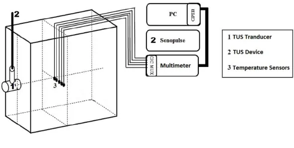
3.3 Schematic diagram of the experiment setup used in the first environment,

homogeneous phantom. Figure adapted [7]. . . 58

3.4 Thermocouple positioning in relation to the TUS device. Figure adapted [7]. . . 59

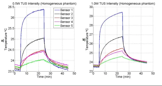
3.5 Temperature recorded by the temperature sensors in the experiment de-scribed in Section (3.3), considering a beam intensity of: a) 0.5W/cm2 and b) 1.0W cm2. . . 60

3.6 Temperature recorded by the temperature sensors in the experiment de-scribed in Section (3.3), considering a beam intensity of: a) 1.5W/cm2 and b) 1.8W cm2. . . 61

4.1 Two distinct phases can be observed in the temperature propagation. Firstly the temperature rises due to the ultrasound being applied to the phantom. After some time, the device is turned off and the phantom cools down naturally. . . 65

4.2 Noise reduction using an 8-point moving average filter. In the figure, data taken from the homogeneous phantom experiment, with a TUS intensity of 1.0W/cm2, exhibits noisy variations in the temperature. . . 66

4.3 Data set collected from the homogeneous phantom experimental setup. TUS Intensity:1.8W/cm2. Sensor: 1. The initial moments clearly exhibit a deficit of data, which can compromise the model learning potential over this region. . . 67

4.4 Results comparison between a model prediction and desired observed val-ues. TUS Intensity:1.0W/cm2. Sensor: 1. The green line represents the absolute error evaluated through all the data set. The effects of the lack of data points are visible, in the initial moments when the temperature is rising rapidly. . . 68

4.5 Interpolation result, applied to the data illustrated in Figure (4.4). The results exhibit a more robust and compact data set, assigning more knowl-edge about the process to the deficient areas. . . 69

4.6 B-spline network design cycle. . . 71

4.7 Data measured by all sensors in the homogeneous phantom with carotid artery experience (1.5W/cm2). . . 73

4.8 Network structure used in SPSI typology models. . . 76

4.9 Network structure used in SPMI typology models. . . 78

4.10 Network structure used in MPMI 1 − D typology models. . . 80

4.11 The angle θ formed between the operating sensor and the TUS central line was chosen to numerically represent the spatial location of the sensor in the 1 − D line. . . 81

4.12 Gaussian distribution with µ = 0 and σ = 0.15. . . 84

4.13 Temperature evolution measured by sensor 2, on the simple homogeneous phantom experiment (1.0W/cm2). The plot illustrates the noise free ver-sion of the signal, in contrast with Figure (4.14), where Gaussian noise was added to the signal. . . 85

4.14 Gaussian noise was added to the previous signal, taken from a normal distribution with µ = 0 and σ = 0.15. . . 85

4.15 Predictive system architecture employing the traditional KTB method. . . 88

4.16 Predictive system architecture employing a neural network ensemble. . . . 89

5.1 Unaltered data set used for SPSI model training, validation and test. Collected from the homogeneous phantom experimental setup. TUS in-tensity: 1.0W/cm2_{. Sensor 1. . . 96}

5.2 Behaviour of model 2 through the whole data set, selected using the KTB approach. The blue line represents the desired behaviour and the model’s training output is given by the black line. The error line is red, circle and cross markers represents the model’s validation and test output respec-tively. SISP,homogeneous phantom experimental setup. TUS intensity: 1.0W/cm2. Sensor 1. Used data: uncorrupted . . . 98 5.3 Data after the addition of random Gaussian noise. The noisy data is used

for training and validation. The unaltered, noise free data is used to test the model. Collected from the homogeneous phantom experimental setup. TUS intensity: 1.0W/cm2. Sensor 1. . . 101 5.4 Behaviour of model 4 in the test set, selected using the KTB approach.

The blue line represents the desired behaviour and the model’s test output is given by the black line. The error line is red. SISP, homogeneous phantom experimental setup. TUS intensity: 1.0W/cm2_{. Sensor 1. Used}

data: corrupted . . . 103 5.5 Data after the addition of random Gaussian noise. The noisy data is used

for training and validation. The unaltered, noise free data is used to test the model. Collected from the homogeneous phantom experimental setup. The top curve corresponds to the strongest intensity. TUS intensity (from the shortest curve to the tallest curve): 0.5W/cm2, 1.0W/cm2, 1.5W/cm2 and 1.8W/cm2. Sensor 1. . . 107 5.6 Behaviour of model 3 in the test set (Sensor 1 0.5W/cm2), selected using

the KTB approach. The blue line represents the desired behaviour and the model’s test output is given by the black line. The error line is red. SIMP, homogeneous phantom experimental setup. Used data: corrupted. . 109 5.7 Behaviour of model 3 in the test set (Sensor 1 1.0W/cm2), selected using

the KTB approach. The blue line represents the desired behaviour and the model’s test output is given by the black line. The error line is red. SIMP, homogeneous phantom experimental setup. Used data: corrupted. . 109 5.8 Behaviour of model 3 in the test set (Sensor 1 1.5W/cm2), selected using

the KTB approach. The blue line represents the desired behaviour and the model’s test output is given by the black line. The error line is red. SIMP, homogeneous phantom experimental setup. Used data: corrupted. . 110 5.9 Behaviour of model 3 in the test set (Sensor 1 1.8W/cm2_{), selected using}

the KTB approach. The blue line represents the desired behaviour and the model’s test output is given by the black line. The error line is red. SIMP, homogeneous phantom experimental setup. Used data: corrupted. . 110 5.10 An example of a trial consisting of 40 temperature data points, divided

between heating and cooling phase. Sampling period T = 60 seconds. Collected from the homogeneous phantom experimental setup. . . 114 5.11 Unaltered data set used for MPMI model training, validation and test.

Collected from the homogeneous phantom experimental setup. Data used: uncorrupted. . . 115

5.12 Top view from the output of model 3 concerning training set (heating phase), selected using the KTB approach. The blue line represents the desired behaviour and the model’s test output is given by the black line. homogeneous phantom experimental setup. The sensors labels just serve as a guidance. The model was constructed using the data illustrated in Figure (E.1). Data division during the model constructed followed thes scheme exposed in Appendix(B), Model 2. . . 115 5.13 Top view from the output of model 3 concerning training set (cooling

phase), selected using the KTB approach. The blue line represents the desired behaviour and the model’s test output is given by the black line. homogeneous phantom experimental setup. The sensors labels just serve as a guidance. The model was constructed using the data illustrated in Figure (5.11). Data division during the model constructed followed thes scheme exposed in Appendix(B), Model 2. . . 116 5.14 Output curve of model 3, selected using the KTB approach, in two

op-erating points embedded in test set (sensor 3, 0.5W/cm2). The blue line represents the desired behaviour and the model’s test output is given by the black line. homogeneous phantom experimental setup. The sensors labels just serve as a guidance. The model was constructed using the data illustrated in Figure (5.11). Used data: uncorrupted. . . 117 5.15 Output curve of model 3, selected using the KTB approach, in two

op-erating points embedded in test set (sensor 4, 1.8W/cm2). The blue line represents the desired behaviour and the model’s test output is given by the black line. homogeneous phantom experimental setup. The sensors labels just serve as a guidance. The model was constructed using the data illustrated in Figure (5.11). Used data: uncorrupted. . . 118 5.16 An example of a trial consisting of 40 temperature data points

contam-inated with Gaussian noise, divided between heating and cooling phase. Sampling period T = 60 seconds. Collected from the homogeneous phan-tom experimental setup. . . 118 5.17 Data after the addition of random Gaussian noise. The noisy data is used

for training and validation. The unaltered, noise free data is used to test the model. Collected from the homogeneous phantom experimental setup. 119 5.18 Top view from the output of model 3 through all the test set (heating

phase), selected using the KTB approach. The blue line represents the desired behaviour and the model’s test output is given by the black line. homogeneous phantom experimental setup. The sensors labels just serve as a guidance. The model was constructed using the data illustrated in Figure (E.4). Data division during the model constructed followed thes scheme exposed in Appendix(B), Model 2. Data used: corrupted . . . 121 5.19 Top view from the output of model 3 through all the test set (cooling

phase), selected using the KTB approach. The blue line represents the desired behaviour and the model’s test output is given by the black line. homogeneous phantom experimental setup. The sensors labels just serve as a guidance. The model was constructed using the data illustrated in Figure (5.17). Data division during the model constructed followed thes scheme exposed in Appendix(B), Model 2. Data used: corrupted . . . 121

6.1 Graphical illustration of the average M SE (test set) calculated for all models typologies, using uncorrupted and Gaussian contaminated data. Solid line: values obtained with uncorrupted data; Dashed line: vales obtained with corrupted data. . . 128 6.2 Graphical illustration of the average LWN calculated for all models

ty-pologies, using uncorrupted and Gaussian contaminated data. Solid line: values obtained with uncorrupted data; Dashed line: vales obtained with corrupted data. . . 130 6.3 Ensemble methods performance enhancements of the various methods

when compared with the KTB paradigm, regarding experiences where the models were build using uncorrupted data. SPSI and SPMI model typology both set 5 discrete points in the plot, whereas MPMI typologies just have one point. This is due to the fact that for the last typology all of the data universe had to be used, resulting in just one possible operating point: all sensors at all TUS beam intensities. . . 134 6.4 Ensemble methods performance enhancements of the various methods

when compared with the KTB paradigm, regarding experiences where the models were build using uncorrupted data. SPSI and SPMI model typology both set 5 discrete points in the plot, whereas MPMI typologies just have one point. This is due to the fact that for the last typology all of the data universe had to be used, resulting in just one possible operating point: all sensors at all TUS beam intensities. . . 135 6.5 Spherical coordinates (r, θ, ϕ) as commonly used in physics: radial

dis-tance r, polar angle θ (theta), and azimuthal angle φ (phi). Taken from [3] . . . 141 A.1 Defining a BS of order 2 through the use of convolution operation. Adapted

from [9] . . . 143 C.1 Uncorrupted original data set used for SPSI model training, validation

and test. Collected from the homogeneous phantom experimental setup. TUS intensity: 1.8W/cm2. Sensor 1. . . 149 C.2 Output curve of model 3 through the whole data set, selected using the

KTB approach. The blue line represents the desired behaviour and the model’s training output is given by the black line. The error line is red, circle and cross markers represents the model’s validation and test out-put respectively. SISP,homogeneous phantom experimental setup. TUS intensity: 1.8W/cm2_{. Sensor 1. Data used: uncorrupted. . . 150}

C.3 Corrupted data after the addition of random Gaussian noise. The noisy data is used for training and validation. The Uncorrupted, noise free data is used to test the model. Collected from the homogeneous phantom experimental setup. TUS intensity: 1.8W/cm2. Sensor 1. . . 153 C.4 Behaviour of model 1 in the test set, selected using the KTB approach.

The blue line represents the desired behaviour and the model’s test out-put is given by the black line. The error line is red. SISP,homogeneous phantom experimental setup. TUS intensity: 1.0W/cm2. Sensor 1. . . 154 C.5 Uncorrupted data set used for SPSI model training, validation and test.

Collected from the homogeneous phantom experimental setup. TUS in-tensity: 0.5W/cm2_{. Sensor 2. . . 158}

C.6 Behaviour of the model 1 through the whole data set, selected using the KTB approach. The blue line represents the desired behaviour and the model’s training output is given by the black line. The error line is red, circle and cross markers represents the model’s validation and test output respectively. SISP,homogeneous phantom experimental setup. TUS intensity: 0.5W/cm2_{. Sensor 2. Data used: uncorrupted. . . 160}

C.7 Data after the addition of random Gaussian noise. The noisy data is used for training and validation. The Uncorrupted, noise free data is used to test the model. Collected from the homogeneous phantom experimental setup. TUS intensity: 0.5W/cm2. Sensor 2. . . 160 C.8 Model’s behaviour in the test set, selected using the KTB approach. The

blue line represents the desired behaviour and the model’s test output is given by the black line. The error line is red. SISP,homogeneous phantom experimental setup. TUS intensity: 0.5W/cm2. Sensor 2. Data used: corrupted. . . 162 C.9 Uncorrupted data set used for SPSI model training, validation and test.

Collected from the homogeneous phantom experimental setup. TUS in-tensity: 1.8W/cm2. Sensor 1. . . 165 C.10 Behaviour of the model through the whole data set, selected using the

KTB approach. The blue line represents the desired behaviour and the model’s training output is given by the black line. The error line is red, circle and cross markers represents the model’s validation and test out-put respectively. SISP,homogeneous phantom experimental setup. TUS intensity: 1.5W/cm2. Sensor 3. . . 166 C.11 Data after the addition of random Gaussian noise. The noisy data is used

for training and validation. The Uncorrupted, noise free data is used to test the model. Collected from the homogeneous phantom experimental setup. TUS intensity: 1.8W/cm2. Sensor 1. . . 168 C.12 Model’s behaviour in the test set, selected using the KTB approach. The

blue line represents the desired behaviour and the model’s test output is given by the black line. The error line is red. SISP,homogeneous phantom experimental setup. TUS intensity: 1.5W/cm2. Sensor 3. Data used: corrupted. . . 170 C.13 Uncorrupted data set used for SPSI model training, validation and test.

Collected from the homogeneous phantom experimental setup. TUS in-tensity: 1.8W/cm2. Sensor 4. . . 173 C.14 Behaviour of the model through the whole data set, selected using the

KTB approach. The blue line represents the desired behaviour and the model’s training output is given by the black line. The error line is red, circle and cross markers represents the model’s validation and test out-put respectively. SISP,homogeneous phantom experimental setup. TUS intensity: 1.8W/cm2. Sensor 4. Data used: uncorrupted. . . 174 C.15 Data after the addition of random Gaussian noise. The noisy data is used

for training and validation. The Uncorrupted, noise free data is used to test the model. Collected from the homogeneous phantom experimental setup. TUS intensity: 1.8W/cm2. Sensor 4. . . 176

C.16 Model’s behaviour in the test set, selected using the KTB approach. The blue line represents the desired behaviour and the model’s test output is given by the black line. The error line is red. SISP,homogeneous phantom experimental setup. TUS intensity: 1.8W/cm2. Sensor 4. Data used: corrupted. . . 178 C.17 Uncorrupted data set used for SPSI model training, validation and test.

Collected from the homogeneous phantom experimental setup. TUS in-tensity: 1.0W/cm2. Sensor 5. . . 181 C.18 Behaviour of the model through the whole data set, selected using the

KTB approach. The blue line represents the desired behaviour and the model’s training output is given by the black line. The error line is red, circle and cross markers represents the model’s validation and test out-put respectively. SISP,homogeneous phantom experimental setup. TUS intensity: 1.0W/cm2. Sensor 5. Data used: uncorrupted. . . 183 C.19 Data after the addition of random Gaussian noise. The noisy data is used

for training and validation. The Uncorrupted, noise free data is used to test the model. Collected from the homogeneous phantom experimental setup. TUS intensity: 1.0W/cm2. Sensor 5. . . 183 C.20 Behaviour of model 3 in the test set, selected using the KTB approach.

The blue line represents the desired behaviour and the model’s test out-put is given by the black line. The error line is red. SISP,homogeneous phantom experimental setup. TUS intensity: 1.0W/cm2. Sensor 5. Data used: corrupted. . . 184 D.1 Corrupted data after the completion of the Gaussian contamination

pro-cess.. The noisy data is used for training and validation. The unaltered, noise free data is used to test the model. Collected from the homogeneous phantom experimental setup. The top curve corresponds to the strongest intensity. TUS intensity (from the shortest curve to the tallest curve): 0.5W/cm2, 1.0W/cm2, 1.5W/cm2 and 1.8W/cm2. Sensor 1. . . 190 D.2 Behaviour of model 4 in the test set (Sensor 2 0.5W/cm2), selected using

the KTB approach. The blue line represents the desired behaviour and the model’s test output is given by the black line. The error line is red. SIMP, homogeneous phantom experimental setup. Data used: corrupted. . 192 D.3 Behaviour of model 4 in the test set (Sensor 2 1.0W/cm2), selected using

the KTB approach. The blue line represents the desired behaviour and the model’s test output is given by the black line. The error line is red. SIMP, homogeneous phantom experimental setup. Data used: corrupted. 192 D.4 Behaviour of model 4 in the test set (Sensor 2 1.5W/cm2), selected using

the KTB approach. The blue line represents the desired behaviour and the model’s test output is given by the black line. The error line is red. SIMP, homogeneous phantom experimental setup. Data used: corrupted. . 193 D.5 Behaviour of model 4 in the test set (Sensor 2 1.8W/cm2_{), selected using}

the KTB approach. The blue line represents the desired behaviour and the model’s test output is given by the black line. The error line is red. SIMP, homogeneous phantom experimental setup. Data used: corrupted. . 193

D.6 Corrupted data after the completion of the Gaussian contamination pro-cess.. The noisy data is used for training and validation. The unaltered, noise free data is used to test the model. Collected from the homoge-neous phantom experimental setup. The top curve corresponds to the strongest intensity. TUS intensity: 0.5W/cm2, 1.0W/cm2, 1.5W/cm2 and 1.8W/cm2_{. Sensor 1. . . . 196}

D.7 Behaviour of model 4 in the test set (Sensor 5 0.5W/cm2), selected using the KTB approach. The blue line represents the desired behaviour and the model’s test output is given by the black line. The error line is red. SIMP, homogeneous phantom experimental setup. Data used: corrupted. . 197 D.8 Behaviour of model 4 in the test set (Sensor 5 1.0W/cm2), selected using

the KTB approach. The blue line represents the desired behaviour and the model’s test output is given by the black line. The error line is red. SIMP, homogeneous phantom experimental setup. Data used: corrupted. 198 D.9 Behaviour of model 4 in the test set (Sensor 5 1.5W/cm2), selected using

the KTB approach. The blue line represents the desired behaviour and the model’s test output is given by the black line. The error line is red. SIMP, homogeneous phantom experimental setup. Data used: corrupted. . 198 D.10 Behaviour of model 4 in the test set (Sensor 5 1.8W/cm2), selected using

the KTB approach. The blue line represents the desired behaviour and the model’s test output is given by the black line. The error line is red. SIMP, homogeneous phantom experimental setup. Data used: corrupted. . 199 E.1 Uncorrupted data set used for MPMI model training, validation and test.

Collected from the homogeneous phantom experimental setup. . . 203 E.2 Model’s behaviour in the test set (Sensor 3 0.5W/cm2_{), selected using the}

KTB approach. The blue line represents the desired behaviour and the model’s test output is given by the black line. The error line is red. MIMP, homogeneous phantom experimental setup. Data used: uncorrupted. . . . 203 E.3 Model’s behaviour in the test set (Sensor 5 1.8W/cm2), selected using the

KTB approach. The blue line represents the desired behaviour and the model’s test output is given by the black line. The error line is red. MIMP, homogeneous phantom experimental setup. Data used: uncorrupted. . . . 205 E.4 Corrupted data obtained after the Gaussian contamination process. The

corrupted data is used for training and validation. The uncorrupted orig-inal data is used to test the model. Collected from the homogeneous phantom experimental setup. . . 206 E.9 Model’s behaviour in the test set (Sensor 1 1.8W/cm2), selected using

the KTB approach. The blue line represents the desired behaviour and the model’s test output is given by the black line. The error line is red. MIMP, homogeneous phantom experimental setup. . . 208 E.5 Model’s behaviour in the test set (Sensor 1 1.8W/cm2), selected using

the KTB approach. The blue line represents the desired behaviour and the model’s test output is given by the black line. The error line is red. MIMP, homogeneous phantom experimental setup. . . 209 E.6 Model’s behaviour in the test set (Sensor 2 1.0W/cm2_{), selected using}

the KTB approach. The blue line represents the desired behaviour and the model’s test output is given by the black line. The error line is red. MIMP, homogeneous phantom experimental setup. . . 209

E.7 Model’s behaviour in the test set (Sensor 1 1.8W/cm2), selected using the KTB approach. The blue line represents the desired behaviour and the model’s test output is given by the black line. The error line is red. MIMP, homogeneous phantom experimental setup. . . 210 E.8 Model’s behaviour in the test set (Sensor 1 1.8W/cm2), selected using

the KTB approach. The blue line represents the desired behaviour and the model’s test output is given by the black line. The error line is red. MIMP, homogeneous phantom experimental setup. . . 210

3.1 Composition of the constructed solution used to resemble human tissue. . 55 5.1 Performance descriptors obtained concerning models with different

num-ber of input lags. The models presented were selected using the KTB approach. SPSI, Sensor 1 (1.0 W/cm2). Used data: uncorrupted . . . 97 5.2 Performance comparison between all methodologies employed (KTB and

ensemble methods). SPSI, Sensor 1 (1.0 W/cm2). Used data: uncorrupted 99 5.3 Generalization error obtained with the ensemble approaches in

compari-son with the KTB model selection. SPSI, Sensor 1 (1.0 W/cm2). Used data: uncorrupted. Notice that a negative value means mitigation of the performance, i.e. the performance got worst. . . 100 5.4 Performance descriptors obtained concerning models with different

num-ber of input lags. The models presented were selected using the KTB approach. SPSI, Sensor 1 (1.0 W/cm2_{). SPSI, Sensor 1 (1.0 W/cm}2_).

Used data: corrupted . . . 102 5.5 Performance comparison between all methodologies employed. SPSI,

Sen-sor 1 (1.0 W/cm2). Used data: corrupted . . . 104 5.6 Generalization error obtained with the ensemble approaches in

compari-son with the KTB model selection. SPSI, Sensor 1 (1.0 W/cm2). Used data: corrupted . . . 105 5.7 Performance descriptors obtained concerning models with different

num-ber of input lags. The models presented were selected using the KTB approach. SPMI (Sensor 1). Used data: corrupted. . . 108 5.8 Performance comparison between all methodologies employed. SPMI

(Sensor 1). Used data: corrupted. . . 111 5.9 Generalization error obtained with the ensemble approaches in

compari-son with the KTB model selection. Used data: corrupted. . . 112 5.10 Performance descriptors obtained concerning models with different

num-ber of input lags. The models presented were selected using the KTB approach. MPMI. Data used: uncorrupted . . . 116 5.11 Performance descriptors obtained concerning models with different

num-ber of input lags. The models presented were selected using the KTB approach. MPMI. Data used: corrupted. . . 120 5.12 Performance comparison between all methodologies employed. MPMI.

Data used: corrupted . . . 122 5.13 Generalization error obtained with the ensemble approaches in

compari-son with the KTB model selection. Data used: corrupted . . . 123

6.1 Average M SE (regarding heating and cooling phases) in test set, cal-culated for all models typologies, using uncorrupted and Gaussian con-taminated data. Section (2.5) briefly explains this performance figure.

. . . 127 6.2 Average linear weight norm obtained at each stage of the typology

uni-verse, regarding models built both with the original and corrupted data sets. . . 130 6.3 Average maximum absolute error obtained at each stage for each model

typology, regarding models built both with the original and corrupted data sets. . . 132 6.4 Average performance enhancements obtained when the various ensemble

methods were applied. Note that these results are obtained in compar-ison with the KTB approach, i.e. the best trained single model. Note that a negative value means a deteoration in the performance, i.e. the performance got worst when compared with the KTB approach, . . . 133 C.1 Performance descriptors obtained concerning models with different

num-ber of input lags. The models presented were selected using the KTB approach. SPSI, Sensor 1 (1.8 W/cm2). Data used: uncorrupted. . . 150 C.2 Performance comparison between all methodologies employed. SPSI,

Sen-sor 1 (1.8 W/cm2). Data used: uncorrupted. . . 152 C.3 Generalization error obtained with the ensemble approaches in

compari-son with the KTB model selection. SPSI, Sensor 1 (1.8 W/cm2_{). Data}

used: uncorrupted. . . 153 C.4 Performance descriptors obtained concerning models with different

num-ber of input lags. The models presented were selected using the KTB approach. SPSI, Sensor 1 (1.8 W/cm2). Data used: corrupted. . . 155 C.5 Performance comparison between all methodologies employed. SPSI,

Sen-sor 1 (1.8 W/cm2_{) . . . 156}

C.6 Generalization error obtained with the ensemble approaches in compari-son with the KTB model selection. SPSI, Sensor 1 (1.8 W/cm2). Data used: corrupted. . . 157 C.7 Performance descriptors obtained concerning models with different

num-ber of input lags. The models presented were selected using the KTB approach. SPSI, Sensor 2 (0.5 W/cm2). Data used: uncorrupted. . . 159 C.8 Performance comparison between all methodologies employed. SPSI,

Sen-sor 2 (0.5 W/cm2_{). Data used: uncorrupted. . . . 161}

C.9 Generalization error obtained with the ensemble approaches in compari-son with the KTB model selection. SPSI, Sensor 2 (0.5 W/cm2). Data used: uncorrupted. . . 162 C.10 Performance comparison between all methodologies employed. SPSI,

Sen-sor 2 (0.5 W/cm2). Data used: corrupted. . . 163 C.11 Generalization error obtained with the ensemble approaches in

compar-ison with the KTB model selection.SPSI, Sensor 2 (0.5 W/cm2). Data used: corrupted. . . 164 C.12 Performance descriptors obtained concerning models with different

num-ber of input lags. The models presented were selected using the KTB approach. SPSI, Sensor 3 (1.5 W/cm2). Data used: uncorrupted. . . 166

C.13 Performance comparison between all methodologies employed. SPSI, Sen-sor 3 (1.5 W/cm2). Data used: uncorrupted. . . 167 C.14 Generalization error obtained with the ensemble approaches in

compari-son with the KTB model selection. SPSI, Sensor 3 (1.5 W/cm2). Data used: uncorrupted. . . 168 C.15 Performance descriptors obtained concerning models with different

num-ber of input lags. The models presented were selected using the KTB approach. SPSI, Sensor 3 (1.5 W/cm2). Data used: corrupted. . . 169 C.16 Performance comparison between all methodologies employed. SPSI,

Sen-sor 3 (1.5 W/cm2). Data used: corrupted. . . 171 C.17 Generalization error obtained with the ensemble approaches in

compari-son with the KTB model selection. SPSI, Sensor 3 (1.5 W/cm2). Data used: corrupted. . . 172 C.18 Performance descriptors obtained concerning models with different

num-ber of input lags. The models presented were selected using the KTB approach. SPSI, Sensor 4 (1.8 W/cm2). Data used: uncorrupted. . . 174 C.19 Performance comparison between all methodologies employed. SPSI,

Sen-sor 4 (1.8 W/cm2). Data used: uncorrupted. . . 175 C.20 Generalization error obtained with the ensemble approaches in

compari-son with the KTB model selection. SPSI, Sensor 4 (1.8 W/cm2_{). Data}

used: uncorrupted. . . 176 C.21 Performance descriptors obtained concerning models with different

num-ber of input lags. The models presented were selected using the KTB approach. SPSI, Sensor 4 (1.8 W/cm2). Data used: corrupted. . . 177 C.22 Performance comparison between all methodologies employed. SPSI,

Sen-sor 4 (1.8 W/cm2). Data used: corrupted. . . 179 C.23 Generalization error obtained with the ensemble approaches in

compari-son with the KTB model selection. SPSI, Sensor 4 (1.8 W/cm2_{). Data}

used: corrupted. . . 180 C.24 Performance descriptors obtained concerning models with different

num-ber of input lags. The models presented were selected using the KTB approach. SPSI, Sensor 5 (1.0 W/cm2). Data used: uncorrupted. . . 182 C.25 Performance comparison between all methodologies employed. SPSI,

Sen-sor 5 (1.0 W/cm2_{). Data used: uncorrupted. . . . 184}

C.26 Generalization error obtained with the ensemble approaches in compari-son with the KTB model selection. SPSI, Sensor 5 (1.0 W/cm2). Data used: uncorrupted. . . 185 C.27 Performance descriptors obtained concerning models with different

num-ber of input lags. The models presented were selected using the KTB approach. SPSI, Sensor 5 (1.0 W/cm2). Data used: corrupted. . . 186 C.28 Performance comparison between all methodologies employed. SPSI,

Sen-sor 5 (1.0 W/cm2_{). Data used: corrupted. . . 187}

C.29 Generalization error obtained with the ensemble approaches in compari-son with the KTB model selection. SPSI, Sensor 5 (1.0 W/cm2). Data used: corrupted. . . 188 D.1 Performance descriptors obtained concerning models with different

num-ber of input lags. The models presented were selected using the KTB approach. SPMI (Sensor 2). Data used: corrupted. . . 191

D.2 Performance comparison between all methodologies employed. SPMI (Sensor 2). Data used: corrupted. . . 194 D.3 Generalization error obtained with the ensemble approaches in

compari-son with the KTB model selection. SPMI (Sensor 2). Data used: corrupted.195 D.4 Performance descriptors obtained concerning models with different

num-ber of input lags. The models presented were selected using the KTB approach. SPMI (Sensor 5). Data used: corrupted. . . 197 D.5 Performance comparison between all methodologies employed. SPMI

(Sensor 5). Data used: corrupted. . . 200 D.6 Generalization error obtained with the ensemble approaches in

compari-son with the KTB model selection. SPMI (Sensor 5). Data used: corrupted.201 E.1 Performance descriptors obtained concerning models with different

num-ber of input lags. The models presented were selected using the KTB approach. MPMI. Data used: uncorrupted. . . 204 E.2 Performance comparison between all methodologies employed. MPMI.

Data used: uncorrupted. . . 206 E.3 Generalization error obtained with the ensemble approaches in

compari-son with the KTB model selection. MPMI. Data used: uncorrupted. . . . 207 E.4 Performance descriptors obtained concerning models with different

num-ber of input lags. The models presented were selected using the KTB approach. MPMI. Data used: corrupted. . . 208 E.5 Performance comparison between all methodologies employed. MPMI . . 211 E.6 Generalization error obtained with the ensemble approaches in

BS Basis Slines

FIR Finite Impulse Response

IIR Infinite Impulse Response

ANN Artificial Neural Netowrks

NN Neural Networks

BSNN Basis Slines Neural Networks

AMN Associative Memory Netowrks

LMS Least Mean Square

ASMOD Adaptive Spline Modelling of Observation Data

NN Neural Networks

MSE Mean Square Error

MA Moving Average

TUS Therapeutic Ultrasound

ERA Effective Radiation Area

NFL Near Field Llength

SPSI Single Point Single Intensity SPMI Single Point Multi Intensity MPSI Multi Point Single Intensity MPMI Multi Point Multi Intensity

MRI Magnetic Resonance Imaging

EIT Electrical Impedance Tomography

BSU Back Scattered Ultrasound

LWN Linear Weight Norm

TSF Time Series Forecasting

KTB Keep The Best

GA Genetic Algorithm

ES Evolutionary Strategy

1

Introduction

1.1

Motivation

The field of thermal therapy has been growing tenaciously in the last few decades. Ther-mal medicine can be defined as the manipulation of the body (or tissue) temperature for the treatment of disease. The application of heat to living tissues is being researched intensely for medical applications, particularly for treatment of solid cancerous tumors using image guidance. Nevertheless thermal therapies are extensively applied in phys-iotherapy, for the treatment of muscle-skeletal problems. Recently the application in oncology has received an increasing attention by the scientists. Oncologic hyperthermia is a technique where the temperature of tumours is raised to values between 43 and 45oC. Hyperthermia can be applied alone or in conjunction with traditional methods, such as the radiotherapy and chemotherapy [10].

A main aspect concerning the application of thermal therapies is the monitoring of tem-perature in the time and space sense, during treatment. A quantitative assessment of temperature is of extreme relevance for both patient security, and for the efficacy of the therapy. Initial approaches make use of invasive measurements, [11] and [12], where the temperature was measured directly at the temperature site. Although it is a precise temperature measurement (the quality of the measurement is highly dependent on the sensor accuracy), this modality suffers from serious problems. Only a limited number of sensors can be placed because there is tissue damage at each sensor placement and in even certain regions it is impossible to place sensors. An insufficient number of sensors can result in a poor spatial resolution.

It has also been pointed that only the methods based on magnetic resonance imaging (MRI) reached the desired resolution for hyperthermia untill now. The referred resolu-tion is a maximum absolute error of 0.5oC/cm3 [13]. Naturally, the major drawback of this approach is the cost associated with MRI instrumentation.

This work proposes a non-invasive approach to monitor the evolution of the temperature during a thermal therapy. Biomedical instrumentation to estimate the temperature in a non-invasive way can benefit from the use of intelligent models to estimate the temperature, by dramatically reducing the costs associated with the practice. This works studies the feasibility of creating predictive models that can estimate, and hence monitor, the tissue’s temperature evolution during a thermal therapy.

1.2

Proposed goals

The main goal of this thesis resides on the creation of predictive models based on B-splines neural networks, which allows to predict the necessary therapy time and the intensity of the ultrasound (most common heating source), according with the charac-teristics of the region intended to heat. Therefore it is needed to:

• Identifying temperature-dependent signal and ultrasonic system features and de-termine the most relevant ones to the system, i.e. which input information should the system have that allows it to accurately estimate the temperature. Increasing

the number of input variables would result in more complex models, therefore a variable should just be introduced as an input if the increase in the prediction performance is justifiable.

• Create predictive b-splines neural network models based on the identified features. These models should be able to effectively estimate the temperature curve evo-lution on the region of interest, i.e. time and space. The benchmark reference is always the MRI standard of 0.5 oC/cm3, which provides a comparison of the results obtained with the current state of art.

• Enhance the system prediction accuracy by applying neural network ensembles methods. Biomedical applications are naturally subject to the most strict con-strains regarding the accuracy of the systems used in the practice of medicine. Therefore any performance enhancement mechanism that can be applied should be studied.

1.3

Thesis outline

This chapter describes the motivation of the work based on main background readings, the proposed goals and summary of the main contributions of this thesis.

Chapter 2 covers all background theory that supports the work developed in this thesis. It starts by defining and representing the problem of predicting temperature propagation. Following this section b-splines are introduced and the structuring of these function to be used as neural networks is also given. We justify why this problem can be solved using such structures. The chapter ends exposing the theory behind neural network ensembles.

Chapter 3 exposes the experimental set-up used in the data acquisition process, which is also characterized. Furthermore this chapter provide a measure of the validity of the data used to construct the models, and it can be used to discuss about how close the environments considered resembles the real, ideal human tissue characteristics.

The modelling methodology and the detailed structure of the models is presented in Chapter (4). This chapter exposes the different temperature predictive models applied in this work. An approach of gradually increasing model complexity was taken while modeling the dynamics of the process. We start by considering models for single-point and single-intensity estimation. Then gradually the complexity of the models is in-creased towards multi-point and multi-intensity estimation. The motivation behind this methodology is due to the interest we have in study and develop insight concerning the feasibility of using BSNN to predict the temperature propagation, in the environments characterized in Chapter(3).

Chapter (5) exposes all of the results obtained Chapter (6) concludes this thesis by providing a global assessment of the predictive models performance. Neural networks ensembles methods are also evaluated in this chapter. Personal thoughts from the au-thor about artificial intelligent field are also presented and the chapter is concluded by pointing out some future research guidance.

1.4

Publications

Currently two publications based on this thesis are being developed, which we leave here for future reference:

• Ferreira, R, Ruano, M.G, Ruano, A.E, Intelligent non-invasive modelling of ultrasound-induced temperature in tissue phantoms. Annals of Biomedical Engineering, Springer, http://www.springer.com/biomed/journal/10439

• Ferreira, R, Ruano, M.G, Ruano, A.E, b-splines neural networks non-invasive mod-elling of ultrasound-induced temperature in tissues. 4th IFAC International

Con-ference on Intelligent Control and Automation Sciences (ICONS 2016). http://icons2016.univ-reims.fr/

2

Background theory

2.1

Introduction

The application intended to develop under the light of this work can be abstracted and crafted in its general form. Going up one abstraction layer, we see from an engineering perspective, a well known problem, namely a time series predicting problem, character-ized in Section(2.2). Section (2.3) deals with the representation of curves, whose study is fundamental to understand basis splines, introduced in Section (2.3.1). In Section (2.4) the problem is observed from a wider context, where the predictive control architecture is introduced. Neural networks (NN) are introduced in Section (2.4.2), with special at-tention to associative memory networks (AMN), Section (2.4.2.1). These structures have a specific organization, on which b-spline neural networks (BSNN) are included, Section (2.4.2.2). The ASMOD algorithm is studied in Section (2.4.2.3). The performance cri-teria applied in this work to assess and compare the predictive models are exposed in

Section (2.5). The optimization of the global predictive system was forced by the use of neural network ensembles, whose theory is covered in Section (2.7) and (2.8).

2.2

Prediction

Generally, the process of prediction can be seen as the forecasting side of information processing, which can be seen as a filtering process. The term filter refers to a device, or an algorithm, that can be used to extract information about a prescribed quantity of interest, from a set of noisy data. Concerning prediction, the aim is to derive information about how the quantity of interest will be like at some time n + N , with N > 0, using data (information) measured up until time n. Observe that the process of prediction is based on experience or knowledge of the process that is required to predict. Essentially a forecast can be obtained by:

1. purely judgmental approaches.

2. causal or explanatory (regression) methods. 3. extrapolative (time series) methods.

4. any combination of the above

We are interested in time series methods, since the available source of information are samples from a process behavior acquired over time.

Predictive modeling is a wide area of study, therefore it is of our interest to develop insight about process to predict, without loss of generality regarding time series. Notice that the propagation of the temperature on a tissue inherently depends on time, hence it can be thought as a time series, thus we are dealing with a time series forecasting (TSF) problem, whose goal consists in learning patterns from historical data in order to predict the behavior of the system, and not how it works.

A time series is defined as a sequence of vectors (or scalars) which depend on time t.

It is pretended to predict the output x(t), of a given process P . The phenomena behind the process may be of discrete or continuous nature. If t is real valued, we are in the presence of a continuous time series, therefore the process needs to be sampled accord-ingly.

With the time series available, we intend to estimate the output of the process P , at some point in the future:

ˆ

x[t + h] = f (x[t], x[t − 1], . . .) (2.2)

We define h as the prediction horizon. For h = 1, the prediction is called one step ahead prediction. If h = n, with n ≥ 2, the prediction is called n step ahead prediction.

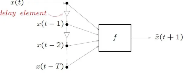
An important observation is that the problem of prediction can be thought as a function approximation problem [14]. A general predictive system is illustrated in Figure (2.1).

Figure 2.1: One step ahead estimation, based on T past values of the process. Adapted from [1].

With respect to the above figure, observe that T delay operations (z−1) are needed, which translates in the need of T storage locations.

Furthermore, the nature of the process must be defined. The process P may be governed by linear dynamics. If so, the problem is in the domain of Digital Signal Processing. The operations carried out on the time series are then be implemented by filters, where two basic architectures are possible: the well known IIR and FIR. However, if the process is governed by non linear dynamics, the problem is a study case of others fields. One of those fields, and the support of this work, consists on Artificial Neural Networks (ANN), structures that provide powerful tools to predict the output of a non linear pro-cess. ANNs are introduced in Section(2.4.2).

As noticed on [14], a forecasting problem can be formulated as a function approximation problem. First of all, the function has to be represented. This can be done in wide variety of formulations. Thus, the mathematical tools for representation of the function must be chosen in accordance with the problem specifications. The definition of this functions is done in the following section.

2.3

Representations of curves

The representation of a curve is a subject of the numerical analysis field, with an exten-sive use in various applications. B-Splines (BS) allow the representation of polynomial parametric curves and have been used in: curve (surface) fitting [15], geometric model-ing [16], identification of non linear [17] systems, control applications [18] and naturally, extensively used in computer graphics applications and CAD systems. Another possible representation of curves can be achieved using Bezier curves [19]. However, B-splines are equipped with more attractive properties as we will see. A parametric representation consists in representing a curve as a function of one (or more) parameter(s):

y(t) : R → Rn, n = 1, 2, 3, . . .

It would be convenient that the function y(t) is as simple as possible, otherwise the evaluation of such function can be computationally expensive. Ideally we are interested in a class of functions which are simple as possible, yet diverse enough to represent a wide variety of curves. To a large extent, polynomial functions satisfy this requirements. A general polynomial function is represented by:

y(t) =

n

X

i=0

aiti (2.3)

where n is the degree of the polynomial and ai the coefficients.

The diversity of curves that one can obtain using polynomials functions is highly depen-dent on the maximum allowed degree. Naturally, the higher the degree, the greater is the flexibility regarding the shape of the curve.

An inflection point is defined as the point on a curve, in which its curvature (second order derivative), changes its signal. A polynomial P (x) of degree n exhibits, at most, n − 1 inflection points. However this high flexibility comes with a cost. The first, and most obvious, relies on the computational complexity, which scales as the degree increases. However, it is also important to observe that the higher degree of a curve, the less controllable it is, in the sense that small changes in coefficients are likely to result in large changes in the shape of the curve, which is a non desirable effect. A small change in a coefficient should, ideally, have its consequences locally constrained, since a local control of the curve is desired in order to have a robust system. To summarize, some commonly desirable properties of curves are:

• C2 _{continuity: The curve should be C}2 _{continuous at all points. Notice that a}

function f (x) is said to be of class Ck if the first k derivatives of f (x) exist and are continuous. This can be seen as a smoothing condition of the curve.

• Interpolation: Should interpolate all of the control points.

• Local control: The modification of a particular control point should modify the curve only locally.

2.3.1 B-Splines

A possible solution to represent curves that meet the previous requirements is to use b(asis)-splines (BSs). BSs were first introduced by Schoenberg in [20]. Originally B-spline basis functions were calculated using a divided difference formula, introduced by

DeBoor in 1978. However the numeric stability of this process sufferd from some restric-tions. Later an important contribution was given by Cox [21], where the author derived an efficient recurrent relationship to evaluate basis functions, which is numerically stable.

To appreciate the usefulness of BSs, notice that any spline function of order k, defined by a set of control points, can be expressed by a linear combination of BSs of the form:

Sk,t(x) =

X

i

αiBi,k(x) (2.4)

Where k represents the order of the spline function, and αi is the associated set of

control points. Bik defines the polynomial pieces, that can be derived by the recursion

algorithm presented on [21]. Note that a linear combination of BSs allows for a flexible construction of curves with a high number of inflection points, showing a smooth and robust behavior to changes of control points. This is done by piecing together several polynomials, as illustrated in Figure (2.2).

Figure 2.2: Piecing polynomials. [2]

However note that the pieces should join continuously at the break point in compliance with the desirable conditions of a curve.

In order to define a BS we need to start with a knot sequence. This sequence should be a non decreasing sequence t := (ti):

Then the BSs of order 1 for this knot sequence, are the characteristic functions of this sequence: Bi1(t) =    1 ti ≤ t < ti+1 0 otherwise (2.6)

The only constraint is that these B-splines should form a partition of unity:

X

i

Bi1(t) = 1, all t (2.7)

Basically, this property assures the invariance of the BS shape under translation and rotational operations. This property is very attractive for geometric applications, which in mathematics is known as affine invariance.

From these first-order BSs, one can obtain high order B-splines by recurrence [21]:

Bi,k = ωi,kBi,k−1+ (1 − ωi+1,k)Bi+1,k−1 (2.8)

with: ωik(t) =        t − ti ti+k−1− ti if ti 6= ti+k−1 0 otherwise (2.9)

Thus, a second order BS is given by:

Bi,2= ωi,2Bi,1+ (1 − ωi+1,2)Bi+1,1 (2.10)

Observing the nature of this recurrent algorithm, one can conclude that a BS of order k consists of polynomial pieces bj,k of exact order k − 1. Note that the second order

BS previously defined, consists of two linear pieces that join continuously to form a piecewise linear function that vanishes outside the interval [ti, . . . , ti+2). Thus, a BS of

order k has support along the interval [ti, . . . , ti+k). Support refers to the region of

the input space where the function assumes non zero values. The number of internal knots must be greater or equal to k − 1. For any interval [ti, . . . , ti+k) at most k of Bi,k

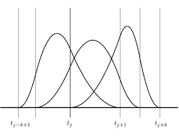
are non zero. This property is illustrated in Figure (2.3), where we can observe three non zero Bi,3 over the interval [tj, . . . , tj+k).

Figure 2.3: Three BS or order 3. Notice the three non zero Bi,3 over the interval

[tj, . . . , tj+k). Adapted from [2]

If in the knot sequence, exists a knot with multiplicity higher than one, the contin-uous condition might be violated in that knot. As an example, consider a BS of order 2. If in the knot sequence exists a knot with double multiplicity, e.g., ti = ti+1, but

still ti+1 < ti + 2, then Bi2 consists of just one piece and fails to be continuous at the

double knot. This is illustrated in Figure (2.4)b), in contrast with a BS of order 2 in which the knot sequence is monotonically increasing, i.e., a sequence just with simple knots, Figure (2.4)a). It is also important to notice that we desire the influence of a control point to be maximum at regions of the curve close to that point, and it should ideally decrease as we move away along the curve, eventually disappearing. Increasing the multiplicity of a knot reduces the continuity of the curve at that knot, i.e., the curve looses smoothness. Generally, a curve its (k − p − 1) times continuously differentiable at a knot with multiplicity p, given that p < k, being k the order of the polynomial. Thus

at that knot, the curve belongs to the class of Ck−p−1 continuity. We can then con-clude that a knot with multiplicity p = k, indicates C−1 continuity, i.e. a discontinuous curve, situation that is not acceptable. The choice of the knot sequence is of major importance in the design phase.

Figure 2.4: BS of order 2 with (a) simple knots, (b) a double knot. Adapted from [2]

For instance consider a B-spline of order 3. A simple knot would mean two smoothness conditions, i.e., continuity of function and first derivative, while a double knot would only leave one smoothness condition, i.e. just function continuity, and a triple knot would leave no smoothness condition, i.e. even the function would be discontinuous. This leads us to the following rule for calculating the order k of the basis function:

k = knot multiplicity + condition multiplicity (2.11)

The following notation can be used to empathize the function dependency on its knot sequence t:

Any smooth piecewise polynomial function is called a spline. If the spline is represented on its B-form, then the spline is described as a linear combination of B-splines:

n

X

j=1

Bj,kaj (2.13)

Therefore a univariate (function of just one variable), spline f , is specified by its non decreasing sequence knot sequence t and by its coefficient sequence ak, which are called

the control points for the curve. The length of the knot sequence t should respect the following rule:

length(t) = n + k (2.14)

Where k is the order and n is the number of B-splines that form the spline function. Furthermore, the order of a BS can be given by:

k = length(t) − na (2.15)

Where na represents the number of control points (coefficients).

Thus the free parameters are the control points and the order of the BS, which pro-vides a B-splines based system a wide flexibility in the design. In contrast with Bezier curves, BS offers a much more localized control, a higher degree of freedom. In Bezier curves a change applied in one point creates a chain of global changes in the whole curve. Also note that the latter offers a less number of free parameters [22], which translates in less flexibility in the system design. Furthermore, the degree of the BS is logically independent of the number of control points. This means the we can use lower degree curves and still maintain a large number of control points.

A more intuitive example can be given in order to better visualize the process behind the construction of a B-spline. Consider a single B-spline of order k = 4 (cubic function), with knot sequence t = [0 1.5 2.3 4 5], a sequence with a length of 5, since we are considering a single B-spline n = 1 of order k = 4 (length(t) = n + k). The graphical representation of the building blocks that constitute the B-spline is shown in Figure (2.5). This figure was generated for illustrative purposes.

Figure 2.5: B-spline of order 4 with knot sequence t = [0 1.5 2.3 4 5]. Each interval, with the respective color, represents one piece of the basis function. Figure generated

with MATLAB, using the Curve Fitting Toolbox [3]

.

The knots are represented by the gray vertical lines. Separation between blocks has been made to empathize the piecing process. Four polynomials of order k − 1 (3) are used in the construction of the basis function, represented by the green, red, violet and black curves. For each interval, formed by two adjacent elements in the knot sequence, a piece (portion) of one of the four k − 1 polynomials is used to form the basis function.

In Figure (2.6) a 6th order BS with the six polynomials of order 5 is presented, which selected pieces (intervals) make up the B-spline.

This figure clearly illustrates the nature of the process behind the constructing of a BS. For a B-spline of order k, specific intervals of order k − 1 polynomials are selected. All of these pieces are joined continuously to form the BS.

Once the basis functions are defined, linearly combining them, weighted by a control point vector ak, gives rise to a spline in its B-form. The short-hand:

f ∈ Sk,t (2.16)

indicates that f is a spline or order k with knot sequence t, i.e, a linear combination of B-splines of order k for the knot sequence t.

Figure 2.6: A 6th order B-spline and the six 5th order polynomials whose selected pieces make up the B-spline. Knot sequence t = [0 1 2 3 4 5 6]. Each piece of the basis function is represented in a different color. Figure generated with MATLAB, using the

Curve Fitting Toolbox [3]

.

The process of constructing a spline by combining basis functions is illustrated in Figure (2.7). This example was constructed to develop insight concerning the local nature of these B-splines.

Figure 2.7: Spline function of order 3, constructed by linearly combining three B-splines of order 3. The blue lines indicate the position of knot, the gray dashed lines represent the B-splines, and the solid black line shows the resulting spline function. Control points employed a = [4 0.3 2.3]. Figure generated with MATLAB, using the

Curve Fitting Toolbox [3]