Univariate and multivariate nonlinear models in productive traits of
the sunn hemp
1Modelos não lineares univariados e multivariados em caracteres produtivos de
crotalária juncea
Cláudia Marques de Bem2*, Alberto Cargnelutti Filho3, Fernanda Carini4and Rafael Vieira Pezzini4
ABSTRACT - Multivariate analysis helps to understand the relationships between dependent variables; this methodology has great potential in several areas of knowledge. The aim of this study was to adjust and compare the univariate and multivariate Gompertz and Logistic nonlinear models to describe the productive traits of sunn hemp ( Crotalaria juncea L.). Two uniformity trials were performed, and the following productive traits were analyzed in 376 sunn hemp plants along 94 days of observations (four plants per day): the fresh mass of leaves (FML), the fresh mass of stem (FMS), and the fresh mass of the aerial parts (FMAP). The Gompertz and Logistic univariate models were adjusted for each productive trait. To adjust the multivariate models, the errors covariance matrix was calculated. The matrix (Cholesky factor) was obtained for each trait, and the multivariate Gompertz (GG) and Logistic (LL) nonlinear models were generated, together with the combination of both models (GL and LG). To define the best model, the residual standard deviation (RSD), the determination coefficient (R2), the Akaike information criterion (AIC), the mean absolute deviation (MAD), and the measures of intrinsic nonlinearity (INL) and parametric nonlinearity (PNL) were calculated. The nonlinear multivariate model LL was adequate and achieved satisfactory results to describe the productive traits of sunn hemp.
Key words: Crotalaria juncea L.. Multivariate analysis. Fresh mass. Growth modeling.
RESUMO - A necessidade de entender o relacionamento entre variáveis dependentes faz da análise multivariada uma metodologia com grande potencial de aplicação em várias áreas do conhecimento. Objetivou-se ajustar e comparar os modelos não lineares univariados e multivariados de Gompertz e Logístico, utilizados na descrição dos caracteres produtivos de crotalária juncea (Crotalaria juncea L.). Foram realizados dois ensaios de uniformidade. Foram avaliados os caracteres produtivos: massa de matéria fresca de folha (MFF), massa de matéria fresca de caule (MFC) e massa de matéria fresca de parte aérea (MFPA), durante 94 dias, sendo avaliadas quatro plantas por dia, totalizando 376 plantas. Os modelos univariados de Gompertz e Logístico foram ajustados para cada caractere produtivo. Para o ajuste dos modelos multivariados, calculou-se a matriz de covariância dos erros. Obteve-calculou-se a matriz (fator de Cholesky) para cada caractere e foram gerados os modelos não lineares multivariados de Gompertz (GG), Logístico (LL) e a combinação de ambos os modelos (GL e LG). Para definição do melhor modelo, utilizou-se o desvio padrão residual (DPR), o coeficiente de determinação (R²), critério de informação de Akaike (AIC), desvio médio absoluto (DMA), medida de não linearidade intrínseca (LI) e medida de não linearidade paramétrica (LP). O modelo não linear multivariado LL foi adequado e obteve resultados satisfatórios para descrever os caracteres produtivos de crotalária juncea.
Palavras-chave: Crotalaria juncea L.. Análise multivariada. Massa de matéria fresca. Modelagem do crescimento.
DOI: 10.5935/1806-6690.20200018 * Author for correspondence
Received for publication 02/04/2019; approved on 20/09/2019
1Este trabalho faz parte do projeto de Pós-Doutorado da primeira autora visando o estudo de uma nova metodologia aplicada aos dados dos caracteres
produtivos da cultura de crotalária juncea. O trabalho foi desenvolvido no Programa de Pós-Graduação em Agronomia da Universidade Federal de Santa Maria/UFSM
2Programa de Pós-Graduação em Agronomia, Departamento de Fitotecnia, Universidade Federal de Santa Maria/UFSM, Santa Maria-RS, Brasil,
[email protected] (ORCID ID 0000-0002-6326-8720)
3Departamento de Fitotecnia, Universidade Federal de Santa Maria/UFSM, Santa Maria-RS, Brasil, [email protected] (ORCID ID
0000-0002-8608-9960)
4Programa de Pós-Graduação em Agronomia, Departamento de Fitotecnia, Universidade Federal de Santa Maria/UFSM, Santa Maria-RS, Brasil, carini.
INTRODUCTION
Sunn hemp (Crotalaria juncea L.) is a fast-growing legume, especially under high temperatures (LEAL et al., 2012). This crop is being increasingly used to suppress weeds development (TIMOSSI et al., 2011). Though being an excellent alternative crop for fresh manure production, it is still scarcely used because there are no data to allow production estimates of this species in Brazil. A promising approach to analyze crop behaviors is the use of nonlinear regression analysis, more precisely, the application of nonlinear regression models (LÚCIO; NUNES; REGO, 2015).
The need to understand the relationships between multiple variables makes nonlinear regression a tool of paramount importance, which can assist in the understanding of biological interactions and the achievement of practical solutions while allowing the characterization of crops’ behavior (REIS et al., 2014). The use of nonlinear regression models provides a comprehensive viewpoint, which may increase the inferences obtained regarding the productive behavior of a given crop throughout its life cycle.
Several statistical models can quantify plant production and describe plant growth patterns, both at the whole-plant level and organ (leaf, stem, and root) level, with nonlinear models being more commonly used (BATES; WATTS, 1988). As the behavior of mass traits presents a sigmoid shape, growth models are recommended for their modeling (SEBER; WILD, 2003). In this context, the Gompertz and Logistic models stand out because they may contribute to or facilitate the interpretation of the processes involved in plant growth, since their parameters allow efficient, practical interpretations (SEBER; WILD, 2003).
Most studies using nonlinear regression models to assess the growth pattern of various crops included a single response variable (univariate models), generating specific models for each variable tested (BEM et al., 2018). Multivariate nonlinear regression models allow the assessment of more than one response variable in a specific experimental unit through the use of a single model (HAIR JÚNIOR et al., 2009), and can, therefore, contribute to a better understanding of the entire crop productive cycle. The designation of “multivariate analysis” comprises a large number of methods and techniques in which all variables are simultaneously used for the theoretical interpretation of a given data set (MOITA NETO, 2004). The purpose of multivariate analysis is to measure, explain, and predict the degree of relationship between different variable combinations, allowing to preserve the natural correlations between the variables without isolating any of them (HAIR JÚNIOR et al., 2009). When
a multivariate technique is used, it is necessary to estimate a significant and representative model of the population under study as a whole, so that reliable results can be obtained (MOITA NETO, 2004). The use of multivariate analysis in agriculture has enabled the comprehension of many complex phenomena and the achievement of valuable answers to several questions, which further became the rationale of different practices. The efficiency of this methodology prompted its widespread application (OLIVEIRA; PADOVANI, 2017). By using multivariate analysis, researchers may obtain deeper knowledge about the productive behavior of sunn hemp, attaining a dynamic approach of fresh aerial mass production throughout the plant cycle.
In previous works, we modeled several sunn hemp productive traits separately using the Gompertz and Logistic univariate nonlinear models (BEM et al., 2018). It may be assumed that the combined analysis of these traits through multivariate nonlinear models could yield a more comprehensive snapshot of this crop, thus contributing to a better understanding of its behavior as a whole. No reports on the calibration of multivariate nonlinear models to study sunn hemp biomass production were found in the scientific literature.
The purpose of this study was to adjust and compare the performance of the univariate and multivariate Gompertz and Logistic nonlinear models to describe the productive traits of sunn hemp as a function of the number of days after sowing.
MATERIALS AND METHODS
The data used were obtained from an experiment conducted in 2014/2015 in the experimental area of the Department of Plant Science of the Federal University of Santa Maria (Rio Grande do Sul, Brazil). Two uniformity trials without treatments (blank experiments) were performed. Sunn hemp seeds were sown in 0.5 m-spaced rows at a density of 20 seeds per row meter in an experimental area of 52 m × 50 m (2,600 m²). The base fertilization was 15 kg ha-1N, 60 kg ha-1P2O5, and
60 kg ha-1K 2O.
After the emergence of sunn hemp seedlings (about seven days after sowing), four plants were collected daily and randomly, totaling 94 days of assessment and 376 plants sampled. The traits evaluated were the fresh mass of leaves (FML, in g plant-1), the fresh mass of stem (FMS,
in g plant-1), and the fresh mass of the aerial parts (FMAP
= FML+FMS, in g plant-1).
The following expression was used for the univariate Gompertz model:
yi = a exp [- exp (b - cxi)] (1)
where a is the asymptotic value; b is the allocation parameter without direct practical interpretation, but important to maintain the sigmoidal shape of the model; and c is the parameter associated with plant growth, which indicates the precocity or maturity index (SEBER; WILD, 2003). The parameter c is the growth rate and represents the velocity with which fresh and dry mass accumulates over time; this velocity can be measured by the second-order partial derivative (MISCHAN et al., 2011; MISCHAN et al., 2015), while xi is the independent variable (days after sowing).
For the univariate Logistic model, the following expression was used:
yi = a/[1 + exp (- b - cxi)] (2)
where a is the asymptotic value; b is the allocation parameter with direct practical interpretation, but important to maintain the sigmoidal shape of the model; and c is the parameter associated with plant growth, which indicates the precocity or maturity index (SEBER; WILD, 2003). The parameter c is the growth rate and represents the velocity with which fresh and dry mass accumulates over time; this velocity can be measured by the second-order partial derivative (MISCHAN et al., 2011; MISCHAN et al., 2015), while xi is the independent variable (days after sowing).
For the univariate Gompertz model, the inflection point (ip) was calculated:
xi = b/c and yi = a/e (3)
the maximum acceleration point (map):
xi = (b - ln (2.62))/c and yi = a * e(-2.62)) (4)
the maximum deceleration point (mdp):
xi = (b - ln (0.38))/c and yi = a * e(-0.38)) (5)
and the asymptotic deceleration point (adp):
xi = (b - ln (0.17))/c and yi = a * e(-0.17)) (6)
using the model parameters a, b, and c, and the constant e = base of the neperian logarithm (2.1782) (MISCHAN; PINHO, 2014). Also, for the univariate Logistic model, the inflection point (ip) was calculated:
xi = -b/a and yi = a/2 (7)
the maximum acceleration point (map):
xi = (-b/c) - (-1/c * 1.3170)) and yi = a/4.7321 (8)
the maximum deceleration point (mdp):
xi = (-b/c) - (-1/c * 1.3170)) and yi = a/1.2679 (9)
and the asymptotic deceleration point (adp):
xi = (-b/c) - (-1/c * 2.2924)) and yi = a/1.1010 (10)
using the model parameters a, b, and c (MISCHAN; PINHO, 2014). These two models were subsequently adjusted for each trait (FML, FMS, and FMAP).
For the adjustment of the multivariate nonlinear models, the residual vector of the univariate nonlinear models was first calculated for each productive trait to obtain the error covariance matrix, from which the matrix (Cholesky factor) for each traits and multivariate model was obtained. Cholesky decomposition is the inverse of the error covariance matrix, given by the
following equation: -1= T , where is an upper
triangular matrix with strictly positive diagonal elements (GALLANT, 1987; FERREIRA, 2011). The new trait for each multivariate model was obtained based on the matrix given by the equation:
yi = p1 * FML + p2 * FMS (11)
The multivariate models tested were the following: GG) Gompertz model for both traits, FML and FMS; LL) Logistic model for both traits, FML and FMS; GL) Gompertz model for FML and Logistic model for FMS; and LG) Logistic model for FML and Gompertz model for FMS. These multivariate models feature the following equations:
GG) yi={a1 exp [-exp b1- c1xi)]} +
{a2 exp [-exp b2- c2xi)]} (12)
LL) yi={a1 exp [-exp b1- c1xi)]} +
{a2 exp [-exp b2- c2xi)]} (13)
GL) yi={a1 exp [-exp b1- c1xi)]} +
{a2 exp [-exp b2- c2xi)]} (14)
LG) yi={a
1 exp [-exp b1- c1xi)]} +
{a2 exp [-exp b2- c2xi)]} (15)
where yi is the new trait (which would correspond to FMAP); a1 and a2 are asymptotic values; b1 and b2 are the allocation parameters without direct practical interpretation, but important to maintain the sigmoidal shape of the model, c1 and c2 are the parameters associated with growth, values that indicate the precocity or maturity index, and xi is the independent variable (days after sowing). In these multivariate models, yi corresponds to the sum of FML and FMS, that is, the FMAP.
In order to verify the goodness of fit of the univariate and multivariate Gompertz and Logistic models, several estimators were calculated. The residual standard deviation (RSD) was determined by the expression:
RSD = √MSE (16)
where MSE = RSS/n-p, and RSS is the residual sum of squares, p is the number of parameters of the model, and n is the number of observations; the best model will be that one which shows the lowest RSD value; the determination coefficient (R²) is given by the expression:
R2 = (1 - RSS)/TSS (17)
where RSS is the residual sum of squares, and
TSS is the total sum of squares; the best model will be
that one which provides the greatest R² value; the Akaike information criterion (AIC) is given by the expression:
AIC = ln (s2) + 2 (p + 1)/n (18)
where (s2) is the logarithm of the errors variance, p is the number of model parameters, and n is the
number of observations; the best model will be that one which presents the lowest AIC value; the mean absolute deviation (MAD) is calculated by this expression: (19)
where yi is the observed value, is the value
estimated by the model, and n is the number of observations; the lower the value, the better the fit of the model.
The use of nonlinear regression models should take into account two aspects to allow the use of parameters as explanatory variables of crop behavior. The degree of intrinsic non-linearity (INL) of the model is the most important one, and is calculated by the expression:
C1 = √F(a;p,n - p) (20)
where p is the number of parameters of the
model; n is the number of observations; and F(a;p,n
- p) is the quantile (α) of the F distribution with p and n - p degrees of freedom. The values must be low to
represent approximately non-biased estimators; values smaller than 0.3 indicate a good linear approximation. Another point is the parametric nonlinearity (PNL) degree, calculated by the expression:
CP = √F(a;p,n - p) (21)
where p is the number of parameters of the model;
n is the number of observations; and F(a;p,n - p) is the
quantile (α) of the F distribution with p and n - p degrees of freedom. Parametric nonlinearity values smaller than 1 indicate a good linear approximation. The smaller the value, the greater the linear approximation of the function (BATES; WATTS, 1988; SEBER; WILD, 2003). All calculations were performed with Microsoft Office Excel® and the statistical software R (R DEVELOPMENT CORE TEAM, 2019).
RESULTS AND DISCUSSION
For the criterion of residual standard deviation (RSD), the lowest values found corresponded to the trait FML adjusted by the Gompertz model and the Logistic model. This result indicates that the observed data points tended to be close to the mean or estimated value. Muianga
et al. (2016) used RSD to evaluate the fit quality of their
nonlinear models to describe cashew fruit growth and stressed the importance of this criterion to evaluate the quality adjustment of statistical models.
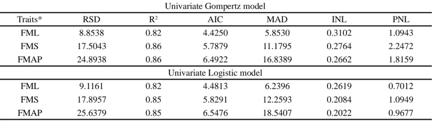
For the univariate Gompertz model, the determination coefficients (R2) ranged from 0.82 to 0.86,
while for the univariate Logistic model, these values ranged from 0.82 to 0.85 (Table 1). These values are considered good, as they are above 0.7. The assessment of the goodness of fit of the models tested through the Akaike information criterion (AIC) and the mean absolute deviation (MAD) revealed differences between models. For the trait FML, the lowest value was found in the Gompertz model. For the traits FMS and FMAP, the results were similar to those found for FML. Therefore, the univariate Gompertz model is that which fits best to the data obtained for productive traits in sunn hemp.
Some studies have emphasized the usefulness of these quality estimators such as that of Reis et al. (2014), who studied garlic accessions groups, as well as that published by Lúcio et al. (2015), who analyzed nonlinear models to predict pumpkin and pepper production and that of Deprá et al. (2016), who evaluated the Logistic model to describe the growth pattern of local corn cultivars and half-sib maternal progenies.
The analysis of the nonlinearity of the models demonstrated an appropriate intrinsic nonlinearity (INL) for both models, as the values found were below 0.3, indicating a good linear approximation. However, for FML, the Gompertz model generated an INL slightly above the optimum (INL=0.3102). In the assessment of the parametric nonlinearity (PNL), for all traits analyzed, this quality indicator was above 1 when the Gompertz model was applied (Table 1), demonstrating a good linear approximation. However, for the Logistic model, the values were below 1 for the traits FML and FMAP.
Table 1 - Fit quality evaluation criteria: residual standard deviation (RSD), determination coefficient (R²), Akaike information criterion (AIC), mean absolute deviation (MAD), degree of intrinsic non-linearity (INL) and parametric nonlinearity (PNL) from univariate models for productive traits fresh mass of leaves, fresh mass of stem, and fresh mass of the aerial parts as a function of days after sowing
Univariate Gompertz model
Traits* RSD R2 AIC MAD INL PNL
FML 8.8538 0.82 4.4250 5.8530 0.3102 1.0943
FMS 17.5043 0.86 5.7879 11.1795 0.2764 2.2472
FMAP 24.8938 0.86 6.4922 16.8389 0.2662 1.8159
Univariate Logistic model
FML 9.1161 0.82 4.4813 6.2396 0.2619 0.7012
FMS 17.8957 0.85 5.8291 12.2593 0.2084 1.0949
FMAP 25.6379 0.85 6.5476 18.5407 0.2022 0.9677
*FML = fresh mass of leaves; FMS = fresh mass of stem; FMAP = fresh mass of the aerial parts (FMAP = FML+FMS)
It should be noted that these nonlinearity estimates are of utmost importance because they indicate how close to linearity the behavior of a nonlinear regression model is. When a nonlinear function is approximately linear, the estimators of the parameters acquire characteristics close to those displayed by the estimators of a linear model. However, when the behavior is not approximately linear, the estimates of the parameters become biased, the confidence intervals are not estimated accurately, and the hypotheses about the statistical parameters cannot be tested (BATES; WATTS, 1988; RITZ; STREIBIG, 2008; SEBER; WILD, 2003). In a study on nonlinear models for hybrid corn seeds germination, Gazola et al. (2011) studied the nonlinearity of the adjusted models. Likewise, in a study on the biological parameters involved in tomato production using a Logistic model SARI et al. (2019), described the importance of nonlinearity measures and they used nonlinearity estimators to evaluate the goodness of fit of their models to describe tomato’s growth pattern. Our results are reliable because they meet the nonlinearity measurements, in this context, the univariate Logistic model yielded better adjustment quality considering the nonlinearity measures (Table 1).
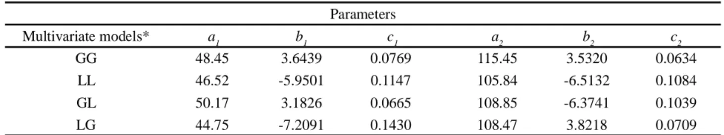
For the adjustment of the multivariate models, the Cholesky factor ( ) was obtained for the combined models GG, LL, GL, and LG, taking into account the traits FML and FMS. The values found in each matrix were subsequently used to obtain the “new” trait, and the multivariate models were adjusted for this “new” trait for the adjustment of the multivariate models GG, LL, GL and LG. Estimate are given below:
GG) Gompertz model for both traits FML and FMS
LL) Logistc model for the both traits FML and FMS
GL) Gompertz model for FML and Logistic model for FMS
LG) Logistic model for FML and Gompertz model for FMS
The criteria of quality adjustment were also calculated for the multivariate models in order to select the best multivariate model able to express the productive traits of the sunn hemp. It can be observed that RSD was similar for all models and lower when compared with the values found for the univariate models, indicating that the points are very close to the average or estimated value; these results can be tested statistically by the F test. In addition, it may be noticed that the multivariate model LL generated the lowest (RSD=0.9952).
The determination coefficients R2 were the
same for all multivariate models tested (Table 2) and lower than those calculated for the univariate models. Notwithstanding, it should be emphasized that these results are also satisfactory, as they all are above 0.7.
The values for the Akaike information criterion (AIC) were similar for the four multivariate models tested, with the lowest value found for the multivariate model LL. It may be appreciated that all these values are smaller as compared with the values found for the univariate models, suggesting the superiority of the multivariate models regarding this evaluation criterion (Table 2). In relation to the criterion MAD, were lower in the multivariate models as compared to the univariate models, ranging between
0.6300 and 0.6456, and yielding the lowest value in the multivariate model GG.
Comparing the MAD values of the multivariate models with the values for the univariate models, it is noted that the values were lower for the multivariate models (Table 2). However, it should be noted that the new “trait” of each multivariate model was constructed based on the Cholesky matrix, and this may have generated interferences. Also, it is important to emphasize that the new trait is composed of the sum of the traits FML and FMS.
As already indicated, the use of quality estimators to assess the goodness of fit of multivariate models is essential when such models will be applied to describe the productive traits of sunn hemp, confirmed the goodness of fit of these models. In this context, it can be concluded that the multivariate models GG and LL are those that fit best to the productive traits of the sunn hemp, taking into account all evaluation criteria of quality adjustment. It should be emphasized that as well as univariate models, the GG and LL multivariate models are appropriate and can be used to adjust the productive traits of sunn hemp, being the multivariate model LL the best one based on the evaluation criteria used in this study, because it was that which yielded the lowest RSD and AIC values, with
identical R2 as compared to the other models and MAD
was the 3º lowest value. Therefore, the conclusion was based on the set of values of these criteria.
Table 2 - Fit quality evaluation criteria: residual standard deviation (RSD), determination coefficient (R2), Akaike information criterion (AIC), and mean absolute deviation (MAD), for the multivariate models GG, LL, GL, and LG for productive traits fresh mass of leaves, fresh mass of stem and fresh mass of the aerial parts as a function of days after sowing
Multivariate models* RSD R2 AIC MAD
GG 1.0047 0.79 0.0568 0.6300
LL 0.9952 0.79 0.0366 0.6456
GL 0.9999 0.79 0.0471 0.6540
LG 1.0002 0.79 0.0474 0.6305
*GG = FML (Gompertz) + FMS (Gompertz); LL = FML (Logístico) + FMS (Logístico); GL = FML (Gompertz) + FMS (Logístico) e LG = FML (Logístico) + FMS (Gompertz)
Few studies highlight the importance of multivariate models to achieve an adequate approach to biological processes. Among them, Teixeira Neto
et al. (2016), described sheep growth using nonlinear
models selected by multivariate techniques and Veloso
et al. (2016), carried out the selection and multivariate
classification of nonlinear models for broiler chickens. It should be emphasized that the higher the number of quality criteria assessed, the more accurate is the identification of the best models (PUIATTI et al., 2013).
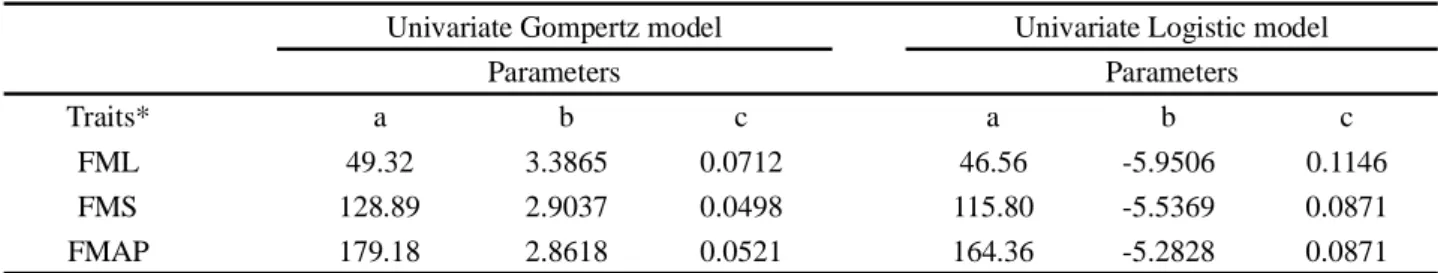
For both the univariate (Table 3) and the multivariate (Table 4) models, the parameters a, b, and
c were calculated. These estimators are relevant since
each parameter has its meaning in the adjustment of these models. The parameter a represents the maximum value that each trait can reach at the end of the sunn hemp productive cycle. Increments in this parameter modify the ordinate’s values, changing, therefore, FML, FMS, and FMAP values. However, the parameter b has no biological interpretation in the Gompertz model, and therefore, does not change trait values. However, in the Logistic model, the parameter b, it has pratical interpretation, in wich the change of values of this parameter interferes with the change of curve concavity. Lastly, increments in the parameter c lead to increases in the slope of the growth curve. The same considerations are valid for the multivariate models.
Table 3 - Estimate of the parameters in the adjustment of productive traits: fresh mass of leaves, stem and aerial parts of sunn hemp
Univariate Gompertz model Univariate Logistic model
Parameters Parameters
Traits* a b c a b c
FML 49.32 3.3865 0.0712 46.56 -5.9506 0.1146
FMS 128.89 2.9037 0.0498 115.80 -5.5369 0.0871
FMAP 179.18 2.8618 0.0521 164.36 -5.2828 0.0871
Table 4 - Estimate of the parameters in the adjustment of productive traits: fresh mass of leaves, stem and aerial parts of sunn hemp Parameters Multivariate models* a1 b1 c1 a2 b2 c2 GG 48.45 3.6439 0.0769 115.45 3.5320 0.0634 LL 46.52 -5.9501 0.1147 105.84 -6.5132 0.1084 GL 50.17 3.1826 0.0665 108.85 -6.3741 0.1039 LG 44.75 -7.2091 0.1430 108.47 3.8218 0.0709
*GG = FML (Gompertz) + FMS (Gompertz); LL = FML (Logístico) + FMS (Logístico); GL = FML (Gompertz) + FMS (Logístico) e LG = FML (Logístico) + FMS (Gompertz)
The multivariate models’ estimates yielded more similar values than the univariate models, the values of these estimates will compose the adjusted equations. The most common way to compare the parameters is by using the F test because it maintains the type I errors at a lower level, even in small samples (REGAZZI; SILVA, 2004). The comparison may also be performed based on the confidence interval of the parameters. Estimator values in our multivariate models indicate that sunn hemp productive traits may be adequately described by these models since these values are close to the values observed.
Univariate models curves display some important points, which help in the practical interpretation of sunn hemp growth pattern. These points are called “influential points” and they comprise the maximum acceleration point (map), the inflection point (ip), the maximum deceleration point (mdp), and the asymptotic deceleration point (adp) (Table 5).
The influential points delimit significant phases in the growth of sunn hemp. The ip determines the time at which the growth rate is maximum, i.e., at this stage, the plants are increasing their fresh mass of leaves and fresh mass of stem at an increasing rate. It should be emphasized that the ip occurs when the crop reaches
Table 5 - Influential points of the univariate Gompertz and Logistic models adjusted for the productive traits: fresh mass of leaves (FML), stem (FMS), and aerial parts (FMAP) of the sunn hemp
map* ip* mdp* adp* map* ip* mdp* adp*
Univariate Gompertz model Univariate Logistic model
FML Xi 28.94 47.60 66.26 80.05 40.37 52.07 63.77 72.44 Yi 10.43 24.69 38.94 44.85 9.86 24.69 36.81 42.39 FMS Xi 31.84 58.28 84.71 104.29 48.45 63.57 78.69 89.89 Yi 27.23 64.44 101.65 117.06 24.47 64.44 91.32 105.17 FMAP Xi 29.66 54.94 80.22 98.95 45.51 60.63 75.74 86.93 Yi 37.86 89.57 141.28 162.72 34.73 89.57 129.61 149.27
*map: maximum acceleration point; ip: inflection point; mdp: maximum deceleration point; and adp: asymptotic deceleration point
half of its productive cycle. The map and mdp are short phases, but they are responsible for approximately 60% of the total leaf and stem fresh mass production (MISCHAN; PINHO, 2014). However, before the map and after the mdp, this production is very slow, because at the map, the plant is beginning its growth, and after the mdp fresh mass accumulation decreases. Finally, at the adp phase, the acceleration of plant growth tends to stabilize towards the end of its production cycle.
For the traits FML, FMS, and FMAP, the adjusted curves are sigmoidal with both the univariate Gompertz model and the univariate Logistic model. These curves represent the behavior of each productive trait throughout the sunn hemp production cycle, therefore the conclusions are achieved individually for each trait. This a disadvantage compared to the adjusted multivariate models (Figure 1).
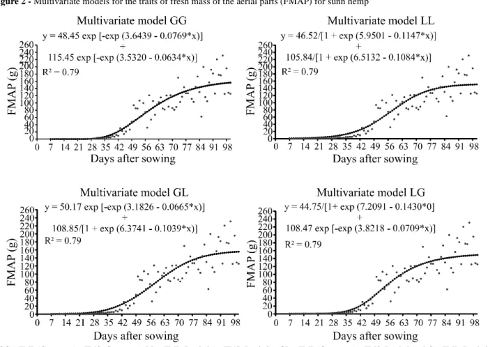
For the multivariate models GG, LL, GL, and LG, composed by the sum of FML and FMS traits equations (FML+FMS=FMAP), a sigmoid growth curve was also observed, providing also a notion of the behavior of the crop along its productive cycle based on the graphical identification of sunn hemp growth phases. Based on these models, it can be concluded that sunn hemp crop attains approximately 140 g of fresh shoot mass at about
Figure 1 - Critical points of the univariate Gompertz model (left column) and univariate Logistic model (right column) for the productive traits: fresh mass of leaves (FML), fresh mass of stem (FMS) and fresh mass of the aerial parts (FMAP) of the sunn hemp
*■ maximum acceleration point; ● inflection point; ▲ maximum deceleration point; asymptotic deceleration point
90 days after sowing. Therefore, these models provide a global view of the sunn hemp cycle, assisting farmers in crop management, as they allow estimating fresh shoot mass production and deciding which is the best harvest time (Figure 2).
Taking into consideration the complete set of criteria used to assess the goodness of fit of the models, the multivariate models GG, LL GL, and LG also yielded satisfactory results for FMAP in sunn hemp, as compared with the univariate models, and therefore are suitable to describe the productive traits of sunn hemp, allowing adequate inferences about total crop production. It is noteworthy that among the
multivariate models here studied, the model that best represented the trait FMAP was the multivariate model LL.
In a previous study with this crop, Bem et al. (2018), fitted the Gompertz and Logistic models for each productive trait and assessed them individually. In the present work, it is demonstrated that GG, LL, GL, and LG multivariate models allow a global vision on the productivity of sunn hemp at the end of the cycle. However, it is necessary to emphasize that these results are specific to this data set, being influenced by the season in which the sunn hemp was sown and the local conditions.
Figure 2 - Multivariate models for the traits of fresh mass of the aerial parts (FMAP) for sunn hemp
* GG = FML (Gompertz) + FMS (Gompertz); LL = FML (Logistic) + FMS (Logistic); GL = FML (Gompertz) + FMS (Logistic) e LG = FML (Logistic) + FMS (Gompertz)
Some published studies also used multivariate analysis to adjust research data: Rosas et al. (2016) estimated coffee productivity using multiple regression, and Bittencourt et al. (2018) determined the productivity features of cotton and soybeans using multiple linear regression models. However, no studies were found on multivariate linear models applied to sunn hemp.
Therefore, the present research is important, since a global conclusion about the crop productivy was obtained and these results may serve as references for future research with sunn hemp.
CONCLUSIONS
1. The present study demonstrates that an overall prediction of sunn hemp productivity can be attained through the use of the multivariate nonlinear models GG, LL, GL, and LG, as they are adequate to describe
the productive traits of sunn hemp and may, therefore, serve as a reference for future research;
2. Additionally, we verified that the nonlinear multivariate model LL, based on the use of the Logistic model for both traits FML and FMS, is the most suitable among the multivariate models tested to describe the productive traits of sunn hemp, under the local conditions under which the experiment was conducted.
ACKNOWLEDGEMENTS
The authors would like to thank the National Council for Scientific and the Tecnological Development (CNPq - Process no. 304652/2017-2) and the Coordination for the Improvement of Higher Education Personal (CAPES) for the financial support to perform this study. The authors also thank the Department of Plant Science of the Federal University of Santa Maria for their support and assistance in conducting the research.
REFERÊNCIAS
BATES, D. M.; WATTS, D. G. Nonlinear regression analysis and its applications. New York: John Wiley & Sons, 1988. 365 p.
BEM, C. M. de et al. Gompertz and Logistic models to the productive traits of sunn hemp. Journal of Agricultural Science, v. 10, n. 1, p. 225-238, 2018.
BITTENCOURT, F. et al. Determinação de funções de produtividade de algodão e soja em cultivo sequeiro no extremo oeste da Bahia. Revista Agroambiental, v. 10, n. 1, p. 67-81, 2018.
DEPRÁ, M. S. et al. Modelo logístico de crescimento de cultivares crioulas de milho e de progênies de meios-irmãos maternos em função da soma térmica. Ciência Rural, v. 46, n. 1, p. 36-43, 2016.
FERREIRA, D. F. Estatística multivariada. 2. ed. Lavras: UFLA, 2011. 676 p.
GALLANT, A. R. Nonlinear statistical models. New York: John Wiley & Sons, 1987. 610 p.
GAZOLA, S. et al. Proposta de modelagem não-linear do desempenho germinativo de sementes de milho híbrido. Ciência Rural, v. 41, n. 4, p. 551-556, 2011.
HAIR JR., J. F. et al. Análise multivariada de dados. 6. ed. Porto Alegre: Bookman, 2009.
LEAL, M. A. A. et al. Desempenho de crotalária cultivada em diferentes épocas de semeadura e de corte. Revista Ceres, v. 59, n. 3, p. 386-391, 2012.
LÚCIO, A. D. C.; NUNES, L. F.; REGO, F. Nonlinear models to describe production of fruit in Cucurbita pepo and
Capiscumannuum. Scientia Horticulturae, n. 193, p. 286-293,
2015.
MISCHAN, M. M.; PINHO, S. Z. et al. Inflection and stability points of diphasic Logistic analysis of growth. Scientia Agricola, v. 72, n. 3, p. 215-220, 2015.
MISCHAN, M. M.; PINHO, S. Z. Modelos não lineares: funções assintóticas de crescimento. 1. ed. São Paulo: Cultura Acadêmica, 2014. 124 p.
MISCHAN, M. M. et al. Determination of a point sufficiently close to the asymptote in nonlinear growth functions. Scientia Agricola, v. 68, n. 1, p. 109-114, 2011.
MOITA NETO, M. J. Estatística multivariada. Revista de Filosofia e Ensino, v. 1, n. 1, p. 1-1, 2004.
MUIANGA, C. A. et al. Descrição da curva de crescimento de frutos do cajueiro por modelos não lineares. Revista Brasileira de Fruticultura, v. 38, n. 1, p. 23-32, 2016.
OLIVEIRA, J. R. T.; PADOVANI, C. R. Análise da inter-relação da produtividade agrícola e características climática na região Sudeste do Estado de Mato Grosso, por técnicas multivariadas. E&S - Engineering and Science, v. 6, n. 2, p. 2-12, 2017.
PUIATTI, G. A. et al. Análise de agrupamento em seleção de modelos de regressão não lineares para descrever o acúmulo de matéria seca em plantas de alho. Revista Brasileira de Biometria, v. 31, n. 3, p. 337-351, 2013.
R DEVELOPMENT CORE TEAM. R: a language and environment for statistical computing. Vienna: R Foundation for Statistical Computing, 2019.
REIS, R. M. et al. Modelos de regressão não linear aplicados a grupos de acessos de alho. Horticultura Brasileira, v. 32, n. 2, p. 178-183, 2014.
REGAZZI, A. J.; SILVA, C. H. O. Teste para verificar a igualdade de parâmetros e a identidade de modelos de regressão não linear. I. Dados no delineamento inteiramente casualizado. Revista de Matemática e Estatística, v. 22, p. 33-45, 2004.
RITZ, C.; STREIBIG, J. C. Nonlinear regression with R. New York: Springer, 2008. 114 p.
ROSAS, J. T. F. et al. Regressão múltipla para estimativa especial da produtividade de café arábica utilizando atributos foliares. Revista Univap, v. 22, n. 40, p. 738-748, 2016. SARI, B. G. et al. Describing tomato plant production using growth models. Scientia Horticulturae, v. 246, p. 146-154, 2019.
SEBER, G. A. F.; WILD, C. J. Nonlinear regression. Hoboken: John Wiley & Sons, 2003. 768 p.
TEIXEIRA NETO, M. R. et al. Descrição de crescimento de ovinos Santa Inês utilizando modelos não-lineares selecionados por análise multivariada. Revista Brasileira de Saúde e Produção Animal, v. 17, n. 1, p. 26-36, 2016.
TIMOSSI, C. P. et al. Supressão de plantas daninhas e produção de sementes de crotalária, em função dos métodos de semeadura. Pesquisa Agropecuária Tropical, v. 41, n. 4, p. 525-530, 2011.
VELOSO, R. C. et al. Seleção e classificação multivariada de modelos não lineares para frangos de corte. Arquivo Brasileiro de Medicina Veterinária e Zootecnia, v. 68, n. 1, p. 191-200, 2016.