Guidance and Robust Control of a double-hull Autonomous Underwater
Vehicle
Carlos Hugo Ribeiro Mendes;[email protected] University of Beira Interior
Cristiano Alves Bentes - [email protected] CEiiA - Centre of Engineering and Product Development
Tiago Alexandre Rebelo - [email protected] CEiiA - Centre of Engineering and Product Development Kouamana Bousson - [email protected] University of Beira Interior
Abstract
The aim of this paper is to present, discuss and evaluate two linear control solutions for an Autonomous Underwater Vehicle (AUV). As guidance solution, a waypoint following and station-keeping algorithm is presented. Then a PID design is proposed, through the decoupling of the linear system into three lightly interactive subsystems. A Linear Quadratic Regulator (LQR) design is also presented, based on the division of the linear system into longitudinal and lateral subsystems. A control allocation law is also presented to deal with the underactuation problems. Both controllers proved robust for this operating point although, regarding performance, and, for the performed simulation, the LQR controller proved more responsive.
Keywords
Linear Quadratic Regulator (LQR); Proportional Integral Derivative (PID); Underwater Vehicle Control; Robust Control; Robust Control
ICEUBI2017 - INTERNATIONAL CONGRESS ON ENGINEERING 2017 – 5-7 Dec 2017 – University of Beira Interior – Covilhã, Portugal
Guidance and Robust Control of a double-hull
Autonomous Underwater Vehicle
Introduction
Autonomous underwater vehicles are unmanned robotic systems whose main goal is to explore the ocean environment. In recent years, the interest in autonomous underwater vehicles has grown, as the technology provides more feasible solutions [1].
CEiiA, an Engineering and Product Development Centre based in Portugal, is currently developing together with its partners a deep sea AUV, (Figure 1) [2]. This AUV follows a double-hull configuration and is capable of reaching a Nominal Diving Depth (NDD) of 3000 meters. Control is achieved via two horizontal and two vertical thrusters. The main goal of this vehicle is to reinforce the national capacity for mobile autonomous deep-sea exploration and monitoring. However, the absence of a human operator narrows down the AUV operations to its control system, computing, and sensing capabilities.
The AUV’s dynamics is inherently nonlinear and time-variant. The uncertain external disturbances difficult controller design. Nonetheless, there are many successfully implemented controllers in this nonlinear environment. Over the years linear theory has evolved to meet control robustness and stability requirements.
This paper proposes two linear control designs that could eventually be implemented on the AUV being developed. First the AUV's dynamic model, derived in [3], is briefly described. After, a waypoint following guidance solution [4] is introduced. As for controller design, PID and LQR methods are applied to the AUV's dynamic model and computationally tested.Then, the results are briefly discussed.
Figure 1 – 3D model of the AUV (courtesy of CEiiA).
Modelling the AUV
Coordinated Frames
To derive the equations of motion that describe the AUV's kinematics, first it is necessary to define two reference frames. The body-fixed {𝑏}, which is the non-inertial frame, is composed of the axes {𝑥𝑏, 𝑦𝑏, 𝑧𝑏}. The local NED (North-East-Down) {𝑛}, the inertial reference frame, is composed of the orthonormal axes {𝑥𝑛, 𝑦𝑛, 𝑧𝑛}.
The Centre of Gravity (CG) and the Centre of Buoyancy (CB) are defined with respect to the 0𝑏, and represented by 𝑟𝑔𝑏 = [𝑥𝑔 𝑦𝑔 𝑧𝑔]𝑇 and 𝑟𝑔𝑏= [𝑥𝑔 𝑦𝑔 𝑧𝑔]𝑇, respectively.
The set of coordinates that expresses position and orientation of the vehicle are defined as: 𝜂 =
x
y
z
T expressed in the {𝑛} frame;For linear velocities and angular velocities (surge, sway, heave, roll, pitch and yaw) the vector is:
𝜈 =
u
v
w
p
q
r
T expressed in the {𝑏} frame;And finally, the control forces and moments vector is: 𝜏 =
X
Y
Z
K
M
N
T expressed in the {𝑏} frame;ICEUBI2017 - INTERNATIONAL CONGRESS ON ENGINEERING 2017 – 5-7 Dec 2017 – University of Beira Interior – Covilhã, Portugal The mathematical equation that represents the dynamics of the underwater vehicle can be derived by the Newton's second law. The resulting relation is given by [5]:
𝑀𝜈̇ + 𝐶(𝜈)𝜈 + 𝐷(𝜈)𝜈 + 𝑔(𝜂) = 𝜏 (1)
where 𝑀 is the inertia matrix including added mass, 𝐶(𝜈) is the Coriolis term including both rigid body and added mass term, 𝐷(𝜈) is the vector of hydrodynamic forces, and 𝑔(𝜂) is the vector of hydrostatic forces. The hydrodynamic data used was derived in [3]. For detailed description about the modeling process of this AUV please refer to [3].
Guidance
This section addresses an extension of the waypoint guidance algorithm of the one presented in [4].
Waypoint and Station-keeping Guidance
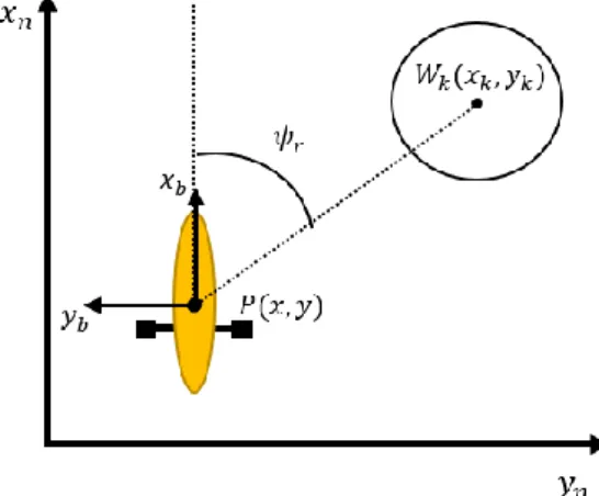
1) Steering Guidance by Line Of Sight:
The LOS guidance algorithm provides a reference angle 𝜓𝑟 that will guide the AUV from its current position towards the waypoint (figure 2). The solution is [6]:
𝜓𝑟= arctan (𝑦𝑘− 𝑦
𝑥𝑘− 𝑥) ∈ −𝜋/2
(2) where 𝜓r is calculated through the four-quadrant version of arctan(𝑦/𝑥) ∈ [−𝜋, 𝜋], usually defined as atan2(𝑦, 𝑥).The waypoint is reached if the vehicle lies inside a Circle Of Acceptance (COA) of radius (𝜌𝑘), around the waypoint. That is [6]:
𝑑𝑘 = √(𝑥𝑘− 𝑥)2+ (𝑦𝑘− 𝑦)2≤ 𝜌𝑘 (3)
where 𝑑𝑘 is the planar distance to the waypoint. Usually [7], 𝜌𝑘 is 2 × 𝐿, where 𝐿 stands for vehicle's length.
Figure 2 – Line Of Sight guidance in the steering plane
2) Reference speed law:
The speed reference is calculated as a function of the distance to the waypoint, 𝑑𝑘, by [4]: 𝑢𝑑= 𝑘𝑢sin−1( 𝑑𝑘
|𝑑𝑘| + 𝑘𝑠) 2
𝜋 (4)
where 𝑘𝑢 is the upper limit of the reference speed and 𝑘𝑠> 0 a parameter for tuning that adjusts the reference speed value according to the distance error. The reference speed never reaches zero because the guidance block will switch for the next waypoint as soon as 𝑑𝑘 ≤ 𝜌𝑘.
ICEUBI2017 - INTERNATIONAL CONGRESS ON ENGINEERING 2017 – 5-7 Dec 2017 – University of Beira Interior – Covilhã, Portugal 3) Diving by Line Of Sight:
Underwater vehicles often control the movement in depth by adjusting pitch. In this case, the vertical common mode can be added to improve depth precision [6]. The reference pitch angle 𝜃𝑟 is given by:
𝜃𝑟= arctan ( 𝑧𝑘− 𝑧
𝑥𝑘− 𝑥) ∈ [−𝜋/2, 𝜋/2] (5)
Since the hydrodynamic data is only valid for 𝜃 values between 20∘ to −20∘ [3], the value of 𝜃 𝑟 follows the same constrains. Special attention to the case where 𝑥𝑘− 𝑥 = 0, which corresponds to the case that the vehicle is already on the planar position (𝑥 = 𝑥𝑘). In this case, the vertical common will bring the AUV to the desired depth.The waypoint acceptance check is now done for both horizontal and vertical coordinates. Therefore, the condition for acceptance becomes:
∣ 𝑧 − 𝑧𝑟∣ | < 𝜌𝑥 ∧ 𝑑𝑘 = √(𝑥𝑘− 𝑥)2+ (𝑦𝑘− 𝑦)2≤ 𝜌𝑘 (6) where 𝜌𝑥 is the depth tolerance, which will be defined as equal to 1 meter.
4) Station-Keeping Mode:
For the final waypoint, the vehicle enters station-keeping mode. This is accomplished by defining the final planar distance as:
𝑑𝑘 = √(𝑥𝑘− 𝑥)2+ (𝑦𝑘− 𝑦)2− 𝜌𝑘 (7)
If 𝑑𝑘𝑓= 0 means that the vehicle is inside the neighbourhood of the last waypoint and only heading control will work. On the other hand, if the vehicle is outside of this neighbourhood the heading and speed control will bring the AUV back.
Control Design
Linearization of the AUV Model
The linear equations can be formulated by linearizing about an equilibrium/operational point (𝜈0, 𝜂0), as in [8]. Defining the state-space as 𝑥 = (𝑥1, 𝑥2)𝑇 where 𝑥1= 𝛥𝑣 = 𝜈 − 𝜈0 and 𝑥2= 𝛥𝜂 = 𝜂 − 𝜂0, the linear equations of motion are given by [8]:
[𝑥̇1𝑥̇2 ] = [−𝑀 −1[𝐶 + 𝐷] −𝑀−1𝐺 𝐽 𝐽∗ ] [ 𝑥1 𝑥2] + [−𝑀 −1 0 ] 𝐮 (8) In many AUV applications, it is reasonable to assume that the AUV is moving with nonzero surge speed, 𝑢0 [8]. It is assumed that the rest of steady state linear and angular velocities are zero, 𝑤0= 𝑣0= 𝑝0= 𝑞0= 𝑟0= 0. For this study, the operating point to be considered is 𝜈0= (0.8,0,0,0,0,0)𝑇.
PID - Proportional Integral Derivative
The Proportional Integral Derivative control will be applied to maximize the manoeuvrability of the AUV. For this AUV it is possible to actively control: surge 𝑢, heading 𝜓, pitch 𝜃 and heave 𝑤. For each, one controller is designed. The roll dynamic, 𝜙, is passively controlled. The Matlab PID tuning tool, from the Control Systems Toolbox, was used for initial gain estimations. Then, by applying the controller to the nonlinear dynamic model, the gains were manually tuned to fit the desired performance. The process can be seen in Figure 3.
ICEUBI2017 - INTERNATIONAL CONGRESS ON ENGINEERING 2017 – 5-7 Dec 2017 – University of Beira Interior – Covilhã, Portugal 1) Speed Controller:
The common mode (𝜏1), i.e. equally dividing the required force by both thrusters, allows the vehicle to control motion in surge. Neglecting interaction with the remaining Degrees Of Freedom (DOFs) [1], the transfer function is given by:
A PI control was applied to the transfer function and tuned. Therefore:
where 𝑢̃ = 𝑢𝑑− 𝑢. To avoid integral windup, the back-calculation method is used. After tuning, since the resulting closed-loop poles are located in the Left Half Plane (LHP), the system is considered stable. The infinity gain margin and the 84.7∘ of phase margin, allied to the fact that the max sensitivity value is below 2 [9], makes the controller robust to disturbances (Figure 4). The respective tracking of a desired velocity can be seen in Figure 5.
Figure 4 - Open- (blue) and closed-loop (black) bode plot for the speed controller.
Figure 5 – Speed controller tracking a reference over time.
1) Heading Controller: 𝑢(𝑠) 𝜏1(𝑠)= 0.0022 𝑠 + 0.0544 (9) 𝜏1= 𝐾𝑝𝑢̃+ 𝐾𝑖∫ 𝑢̃(𝜏)𝑑 𝑡 0 𝜏 (10)
ICEUBI2017 - INTERNATIONAL CONGRESS ON ENGINEERING 2017 – 5-7 Dec 2017 – University of Beira Interior – Covilhã, Portugal Heading control is accomplished through the differential mode (𝜏6), i.e. dividing the required moment by both thrusters. For this subsystem, the state variables to account for are: 𝑣(𝑡), 𝑟(𝑡) and 𝜓(𝑡). For the above mentioned operating point, the result is:
6
0
0.0037
0.0003
0
1.0000
0
0
0.0441
0.4979
0
0.4037
0.3108
=
r
v
r
v
(11)The transfer function for this subsystem is: 𝜓(𝑠) 𝜏6(𝑠)
= 0.003729𝑠 + 0.0009888 𝑠3+ 0.3549𝑠2+ 0.2147𝑠
(12) Heading measurements (𝜓) may be given by compass readings and the yaw rate (𝑟) by a gyroscope. A PD controller provides good performance. The derivative term provides additional phase margin, which increases robustness [1]. The control law yields:
𝜏6= 𝐾𝑝𝜓̃ − 𝐾𝑑𝑟 (13)
where 𝜓̃ = 𝜓𝑟− 𝜓. Special attention to the yaw error. It must be redefined, as in [4]: if 𝜓̃ > 𝜋 (right side)
𝜓̃ = 𝜓̃ − 2𝜋 if 𝜓̃ < −𝜋 (left side)
𝜓̃ = 𝜓̃ + 2𝜋
(14)
The closed-loop poles, for the closed-loop transfer function, are located in the LHP, meaning once more that that the controller is stable. The infinity gain margin and the 84.9∘ of phase margin of the open loop system translates into robustness to disturbances.
2) Depth Controller:
Depth control presents a common mode (𝜏3) and a differential mode (𝜏5). The associated state variables are: 𝑤(𝑡), 𝑞(𝑡), 𝜃(𝑡) and 𝑧(𝑡). Once more, for this operating point, the state-space form yields:
5 30
0
0
0
0.0034
0.0003
0.0003
0.0012
0
0
0
1.0000
0
0
1.0000
0
0
1.0902
0.3070
0.7934
0
0.0974
0.4482
0.2604
=
z
q
w
z
q
w
(15)The diving manoeuvre will be accomplished by adjusting pitch. Through the differential mode (𝜏5) the controller will approach the 𝜃𝑟 angle. To maneuver/adjust the vehicle to the desired depth, as to cancel the residual buoyancy, the common mode (𝜏3) is used. The transfer function of depth is:
𝑧(𝑠) 𝜏3(𝑠)=
0.00119𝑠2+ 0.0002308𝑠 + 0.001268
𝑠4+ 0.5675𝑠3+ 1.526𝑠2+ 0.3612𝑠 (16)
The controller is designed without integral action according to: 𝜏3= 𝐾𝑝𝑧̃+ 𝐾𝑑
𝑑𝑧̃
𝑑𝑡 (17)
where 𝑧̃ = 𝑧𝑟− 𝑧. Once more the infinity gain margin and the 82.2∘ of phase margin of the open loop system shows that the system is robust to disturbances.
ICEUBI2017 - INTERNATIONAL CONGRESS ON ENGINEERING 2017 – 5-7 Dec 2017 – University of Beira Interior – Covilhã, Portugal The transfer function for pitch is:
𝜃(𝑠) 𝜏5(𝑠)
= 0.003362𝑠 + 0.001114
𝑠3+ 0.5675𝑠2+ 1.526𝑠 + 0.3612 (18)
Implementing a PID controller:
𝜏5= 𝐾𝑝𝜃̃+ 𝐾𝑖∫ 𝜃̃(𝜏)𝑑𝜏 𝑡 0 + 𝐾𝑑 𝑑𝜃̃ 𝑑𝑡 (19)
where 𝜃̃ = 𝜃𝑟− 𝜃. An infinity gain margin and the 96.7∘ of phase margin shows robustness of the system.
LQR – Linear Quadratic Regulator
To derive the Linear Quadratic Regulator control law, controllability and observability need to be ensured [10]. Considering a linear model, 𝑥̇ = 𝐴𝑥 + 𝐵𝐮, and that all states are available for the controller, the optimal control problem determines the feedback gain for the optimal control vector [11]:
𝐮(𝑡) = −𝐾(𝑥 − 𝑥𝑑𝑒𝑠𝑖𝑟𝑒𝑑) (20)
The process used to design the controllers is represented in Figure 6. The complete linear system is divided into two subsystems: lateral subsystem and longitudinal subsystem.
1) Longitudinal Controller:
The longitudinal controller is dedicated to control the surge speed (𝜏1) and depth (𝜏3 for the common mode and 𝜏5 for the differential mode). The sate vector is constituted by the states: 𝑢, 𝑤, 𝜃 and 𝑧. For the longitudinal state vector 𝑥𝐿, the state and input matrices from the linearized model for the longitudinal controller are:
[ 𝛥𝑢̇ 𝛥𝑤̇ 𝛥𝑞̇ 𝛥𝜃̇ 𝛥𝑧̇ ] = 𝐴𝐿𝑥𝑙+ 𝐵𝐿𝐮𝐿 = 𝐴𝐿 [ 𝑢 − 𝑢0− (𝑢𝑑− 𝑢0) 𝑤 − 𝑤0 𝑞 − 𝑞0 𝜃 − 𝜃0− (𝜃𝑟− 𝜃0) 𝑧 − 𝑧0− (𝑧𝑑− 𝑧0) ] + 𝐵𝐿𝐮𝐿 (21)
To reduce the steady state values of 𝑢 and 𝜃, two integrative states were added to the state-space: 𝑥∫ 𝑢= ∫ (𝑢 − 𝑢𝑑)𝑑𝜏 𝑡 0 ; (22) 𝑥∫ 𝜃= ∫ (𝜃 − 𝜃𝑟)𝑑𝜏 𝑡 0 ; (23)
ICEUBI2017 - INTERNATIONAL CONGRESS ON ENGINEERING 2017 – 5-7 Dec 2017 – University of Beira Interior – Covilhã, Portugal Therefore, the new state-space equation is:
[ 𝑥̇𝐿 𝑥̇∫ 𝑢 𝑥̇∫ 𝜃 ] = [ 𝐴𝐿 05×2 [1 0 0 0 0 0 0 1 0 0] 02×2 ] [ 𝑥𝑙 𝑥∫ 𝑢 𝑥∫ 𝜃 ] + [ 𝐵𝐿 01×3 01×3 ] 𝐮𝐿 (24)
Because there is an output limitation, the actuators will most likely saturate, inducing once again integral windup. The anti-windup method described in [12] is applied.
2) Lateral Controller:
The main purpose of the lateral system is to control the yaw angle 𝜓. As in the PID heading control, the state vector is constituted by the states: 𝑣, 𝑟 and 𝜓. Assuming the state-space vector of the lateral subsystem as 𝑥𝐻, the state and input matrices from the linearized model will be: [ Δ 𝑣̇ Δ 𝑟̇ Δ 𝜓̇ ] = 𝐴𝐻𝑥𝐻+ 𝐵𝐻𝐮𝐻 𝑥𝐻= 𝐴𝐻[ 𝑣 − 𝑣0 𝑟 − 𝑟0 𝜓 − 𝜓0− (𝜓𝑑− 𝜓0) ] + 𝐵𝐻𝐮𝐻 (25)
The control input is defined as:
𝐮𝐻= −𝐾𝐻𝑥𝐻 (26)
The operating point is the same as in PID. By defining the performance index in terms of the output vector, the Q matrix will only contain the element that dictates the evolution of the output [5]. The resulting eigenvalues of the closed-loop systems (𝑒𝑖𝑔(𝐴𝐻− 𝐵𝐻𝐾𝐻)) are negative which according, to Lyapunov [13], proves that the system is stable. With respect to stability margins, the LQR is known to have excellent stability characteristics with gains up to infinity and phase margin over 60∘ [14].
Control Allocation
Both of PID and LQR use a differential mode, 𝜏6, and a common mode, 𝜏3, through separate laws. This means that the two laws will compete for control authority. Without accounting for thrust constrains, this solution will lead to actuator saturation, resulting in poor performance and instability [15]. The control allocation law from [15] is adapted to solve this problem. Considering now the new common mode law, 𝜏1′:
𝜏1′= 𝜏1𝑒−𝛽∣𝜏6∣ (27)
where 𝜏1 is the control signal determined by the speed controller, 𝛽 is user-set and dependent on the desired fraction of commanded surge, and 𝜏6 the control signal determined by the heading controller.
Simulation Results
Waypoint and Station-keeping
For simulation purposes, the selected waypoint coordinates are defined in table 1. The thrust output was limited at 120 N, in forward thrust, and 85 N in reverse thrust. Thruster dynamics were not considered. However, this should have an overall minor effect on the simulation results.
Table 1 – Waypoint coordinates.
Waypoint 1 Waypoint 2 Waypoint 3 Waypoint 4
x [m] 10 40 50 80
y[m] 20 20 50 60
ICEUBI2017 - INTERNATIONAL CONGRESS ON ENGINEERING 2017 – 5-7 Dec 2017 – University of Beira Interior – Covilhã, Portugal
Conclusions
This paper briefly describes a guidance waypoint and station-keeping algorithm and two control solutions for three AUV autopilots: heading, speed and depth.
Both LQR and PID controllers proved robust for this operating point. For robustness and stability analysis bode was used. The phase margin above 60° and the gain margin up to infinity, allied to the maximum sensitivity values bellow 2, for all autopilots proved robustness of PID and LQR controllers.
Both controllers behaved satisfactorily. However, from the results in Figure 7, it is possible to conclude that the responsiveness of the LQR is greater than the PID’s.
The control allocation law proved to reduce the overshoot on the waypoint, by prioritizing heading over velocity. For that reason, manoeuvrability was increased and COA had to be reduced to a minimum value. Otherwise the vehicle would switch to the next waypoint without reaching the current one.
It is intended, as a continuation of this work, to verify and validate the controllers through further analysis and tests. Further PID tuning could lead to a better performance. Also, the impact of ocean currents should be studied.
Figure 7 - LQR (full line) and PID (dashed line) results for the simulation. The top figures regard the spatial evolution of the vehicle in the vertical (left) and horizontal (right) planes. The bottom figures regard the evolution of the vehicle in the East (left) and Down (right) coordinates over time.
ICEUBI2017 - INTERNATIONAL CONGRESS ON ENGINEERING 2017 – 5-7 Dec 2017 – University of Beira Interior – Covilhã, Portugal
Acknowledgments
This research work was conducted at CEiiA and in the Laboratory of Avionics and Control (Department of Aerospace Sciences) of the University of Beira Interior. The underlying research activities were supported by CEiiA and by the Aeronautics and Astronautics Research Group (AeroG) of the Associated Laboratory for Energy, Transports and Aeronautics (LAETA).
References
[1] B. Jalving, “The ndre-auv flight control system,” IEEE Journal of Oceanic Engineering, 2002.
[2] “Medusa deep sea.” [Online]. Available: http://www.medusadeepsea.com/
[3] C. A. Bentes, “Modeling of an autonomous underwater vehicle,” Master’s thesis, University Of Beira Interior, 2016.
[4] J. Ribeiro, “Motion control of single and multiple autonomous marine vehicles,” Master’s thesis, Instituto Superior Técnico, 2011.
[5] T. I. Fossen, Handbook of Marine Craft Hydrodynamics and Motion Control. John Wiley & Sons, 2011.
[6] V. Bakaric, Z. Vukic, and R. Antonic, “Improved line-of-sight guidance for cruising underwater vehicles,” IFAC Proceeding Volumes, vol. 37, pp. 447–452, 2004.
[7] A. J. Healey and D. Lienard, “Multivariable sliding mode control for autonomous diving and steering of unmanned underwater vehicles,” IEEE journal of Oceanic Engineering, vol. 18, no. 3, pp. 327–339, 1993.
[8] L. Moreira and C. G. Soares, “H2 and H∞ designs for diving and course control of an
autonomous underwater vehicle in presence of waves,” IEEE Journal of Oceanic Engineering, 2008.
[9] K. J. Åström and T. Hägglund, PID controllers: theory, design, and tuning, vol. 2. Isa Research Triangle Park, NC, 1995.
[10] K. Ogata, Modern Control Engineering. Instrumentation and controls series, Prentice Hall, 2010.
[11] M. S. Triantafyllou and F. S. Hover, Maneuvering and Control of Marine Vehicles. Massachusetts Institute of Technology, 2003.
[12] C. M. R. Oliveira, M. L. Aguiar, W. C. A. Pereira, A. G. Castro, T. E. P. Almeida, and J. R. B. A. Monteiro, “Integral sliding mode controller with anti-windup method analysis in the vector control of induction motor,” in 2016 12th IEEE International Conference on Industry
Applications (INDUSCON), 2016.
[13] J. Slotine and W. Li, Applied Nonlinear Control. Prentice-Hall International Editions, Prentice-Hall, 1991.
[14] W. Naeem, Guidance and Control of an Autonomous Underwater Vehicle. phd, Univeristy of Plymouth, 2004.
[15] I. R. Bertaska and K. D. von Ellenrieder, “Supervisory switching control of an unmanned surface vehicle,” in OCEANS 2015 - MTS/IEEE Washington, pp. 1–10, 2015.