Eric Conrado de Souza
[email protected] Centro Universitário da FEI Dept. de Eng. Mecânica 09850-901 São Bernardo do Campo, SP, BrazilNewton Maruyama
[email protected] Escola Politécnica da Univesidade de São Paulo Dept. de Eng. Mecatrônica e de Sist. Mecânicos 05508-900 São Paulo, SP, Brazilµ
-Synthesis for Unmanned Underwater
Vehicles Current Disturbance
Rejection
This note focuses attention on a novel approach to disturbance rejection when the µ-synthesis control procedure is applied to Unmanned Underwater Vehicles (UUVs). Environmental external disturbances simplify to ocean current for a totally submerged vehicle and greatly contributes for hydrodynamical loads and the tether cable disturbance. Our case scenario deals with the incorporation of the sea current disturbance to the plant model employed for control design. In the proposed design method, we substitute the structured unmodeled dynamics uncertainty, which is generally difficult to come up with and eventually utilized to represent external disturbances, by parametric uncertainty, relatively easier and straightforward to come by. The sea-current load parameters are, therefore, treated as parametric uncertainty and fit in the µ design framework. Assuming that both vehicle motion and current direction lie in the horizontal plane, the incoming (to vehicle) current vector sets a horizontal circumference sector in which it may vary. When in the 3D space, current uncertainty renders a cone in space. For validation purposes, the linear controller is simulated with the nonlinear vehicle model.
Keywords: mobile robots, robust control, nonlinear control systems
Introduction1
The success of controlling a dynamical system is directly connected to the designer's ability on determining the relevancy of present uncertainty and on obtaining, thereafter, an estimate of what is not or is poorly known. The resulting uncertainty model if unstructured may yield conservative designs by leaving out desired performance. Obtaining an uncertainty model can be an exhaustively difficult task in general, even for structured uncertainty.
Unmanned Underwater Vehicles (UUV) have been extensively utilized over the years due to increasing interest in the underwater environment. One variant of such vehicles, the Autonomous Underwater Vehicles (AUV), is endowed with features which enable them to work autonomously from human assistance. Earlier results on UUV control design, such as those in Campa et al. (1998), point out relevant issues in regard to structured uncertainty modeling for AUVs and compare sliding-mode and µ-synthesis control results. Some uncertainty modeling details, however, remain unclear. An integrated guidance and gain-schedule control design strategy for AUVs was addressed in Fryxell et al. (1996). In a recent study (Feng and Allen, 2004), reduced order robust SISO controllers were designed for AUV speed, heading, and depth control via the LMI approach. Souza et al. (2004), the LQG/LTR robust multivariable linear control technique, applied for AUV dynamical positioning, considered unmodeled dynamic uncertainty and parametric plant perturbation dealt with by the same control specification, which could render a conservative design. In addition, specifying unmodeled dynamics, even if structured, may not prove to be an easy task. To overcome this difficulty, this note focuses attention on transforming what could be considered external disturbance into “easily” modeled parametric perturbation.
The following developments below will restrict attention to AUV class systems, for which no tether cable to the surface is present as seen on Remotely Operated Vehicles, or ROVs. In this case, given a totally submerged vehicle, and for adequate buoyancy and gravity compensation, the environmental external disturbances simplify to the hydrodynamical loads induced by ocean current. The
µ-synthesis control method is applied for vehicle velocity control.
Disturbance rejection is exchanged to plant model perturbation
Paper received 1 April 2009. Paper accepted 18 January 2010. Technical Editor: Paulo Miyagi
through the incorporation of the sea current disturbance to the plant model employed for control design.
In the proposed design approach we substitute the structured uncertainty due to unmodeled dynamics, which is generally difficult to come up with and eventually utilized to represent external disturbances, by structured parametric uncertainty, relatively easier and straightforward to come by. The sea-current load parameters are, therefore, treated as parametric uncertainty and fit in the µ design framework. Two principal case studies are discussed; one of which is implemented. System sensitivity with respect to the underlying uncertainty parameter spaces may be verified according to these two cases. For validation purposes, the linear controller is simulated with the nonlinear vehicle model.
This text is organized as follows. At first, system modeling is addressed. A brief overview of the µ-synthesis control strategy is then presented. In the following section, a few controller design issues are considered and some synthesis results are depicted. A quick discussion on fundamental issues such as stability, performance and computational implementation is also made. Simulation results are presented. Finally, concluding remarks are drawn based on what has been presented, and a short review for future implementations is presented.
Nomenclature
G = linearized dynamic system model K = linear controller
M = generalized mass matrix
P(s) = augmented plant transfer function
F(i)(A,B) = LFT of A and B. i = {l(lower), u(upper)}.
Greek Symbols
η = position/attitude vector in inertial coordinate frame,
T
z y
x, , , , , ] [ φ θ ψ
η =
ν = velocity vector in body coordinate frame
6 ] , , , , ,
[uvw pqrT∈R
= ν
νc = current velocity vector in body coordinate frame τ = system input vector in body coordinate frame
6 ] , , , , ,
[X Y Z K M N T∈R
Eric Conrado de Souza and Newton Maruyama
Subscripts
A = relative to Added mass dynamics
RB = relative to Rigid Body dynamics c = relative to current
System Modeling
Underwater vehicle modeling
The model used in the following discussion is based on the MURS 300 Mark II ROV (Ishidera et al., 1986). Although our discussions are AUV oriented, control design is realized with the MURS 300 vehicle model due to its complete hydrodynamical drag coefficient data available. This assertion is supported by the fact that we will be restricting our model based control design to relatively low velocities and, so, ROV and AUV dynamics can be considered similar, when neglecting ROV tether cable loads. The MURS 300 vehicle is nearly neutrally buoyant and controllable on all six degrees-of-freedom (dof). It is propelled by six thrusters distributed longitudinally two-by-two on each body axis. A full order mathematical model has been developed, i.e., all six dof are considered. The underwater vehicle nonlinear and coupled dynamics can be modeled by the following expression (Kalske and Happonen, 1991; Fossen, 1994; Souza, 2003):
τ τ η ν
ν
ν+C +FD vr +G = c+
M& ( ) ( ) ( ) , (1)
ν η
η&=J( ) (2)
where
A RB M M
M= + and C=CRB+CA (3)
The generalized mass matrix M accounts for vehicle inertia matrix MRB and the added (A) mass inertia matrix MA, taken as
diagonal. It is important to note that added mass coefficients may be considered constant for a totally submerged vehicle at depths where the influence of waves is minimal. Likewise, the centripetal and Coriolis forces matrix C is computed from the rigid body centripetal and Coriolis forces matrix CRB, derived from rigid body (RB)
dynamical expressions, and from the corresponding added mass
forces matrix CA, which derives from Kirchhoff's equations, see
Fossen (1994). The term FD(νr) stands for nonlinear hydrodynamic
damping action, or drag. Observe from Eq. (1) that the hydrodynamic drag is a function of the relative velocity νr, which is
obtained by the vehicle orientation with respect to fluid motion or current νc. That is:
C r ν ν
ν = − (4)
The hydrodynamic coefficients in FD(νr) also vary with the vehicle
state and current orientation. Lift force components are considered negligible for non-wing like vehicles and when restricted to operation with moderate velocity profiles. Restoring forces and moments are accounted for in G(η), comprising gravitational weight
and buoyancy components. Unrelated drag, current disturbance is given by τc and other environmental phenomena are not considered.
For neutrally buoyant vehicles with homogeneously distributed mass, Eq. (1) may be rewritten with respect to the relative velocity
νr by switching τc to the left side of the equation and plugging it to
the vehicles dynamics into Mν&and C(ν)ν. System input is denoted by the τ force vector. The J matrix indicates when coordinate
transformation is made between the inertial and mobile reference frames, see Fig. 1.
Model linearization
The velocity vector ν is chosen as the system new state vector x.
The UUV linear system dynamics was obtained by classical or Jacobian linearization around nominal state values for linear velocity ν1* = [1.0; 0.1; 0.1] m/s and angular velocity ν2* = [0.1; 0.1; 0.1] rad/s. Furthermore, as will be explained later, the current
magnitude and direction are treated as system parameters and affect the linear model. For a 1 m/s magnitude current vector in the opposite direction to surge, the linear model found was stable. However, taking the current vector aligned in the surge direction, the linear model rendered two slightly unstable modes, given that current tends to accelerate the vehicle. Linearization yielded the state matrix A and the input matrix B used in the control framework
detailed below. System output y was chosen to reflect the velocity
vector ν and, hence, full state feedback is considered, making the system observable. The resulting linear system is minimum phase, and was tested and confirmed for controllability.
Figure 2. Two possible case studies.
Variable scaling
This procedure may be carried out by employing expected maximum values for the output y (= ν) and the input u (= τ) of the
linear system model G(s) in the following manner:
u norm s S yG sS G
s
G( )= ( )= −1 ( ) . (5)
The entries for the scaling matrices Sy and Su are usually
obtained by employing nominal or maximum expected values for the output ν and the input τ variables. In this case, the scaling matrices are given as:
}, , , , , ,
{umax vmax wmax pmax qmax rmax diag
Sy= (6)
}. , , , , ,
{Xmax Ymax Zmax Kmax Mmax Nmax
diag u
S = (7)
A direct consequence of this normalization translates to the minimization of the condition number, i.e., the ratio of the system largest to the smallest singular values is led to a value close to one, for the frequency range of interest. Instead of considering variable scaling by maximum values, the scaling procedure was obtained by fully automating a search process, in the frequency domain, by iterating the scaling matrices. Nominal or maximum output and input entries may be used as a boundary condition. The search algorithm stops when the local minimum is found. This procedure was found to be more efficient than the former alternative.
Uncertainty characterization
The proposed approach for current disturbance rejection considers the modeling assumption described in the System Modeling section, except that instead of writing the overall vehicle dynamics with respect to the relative velocity νr, the current
velocity dependent terms are considered as system parameters that may vary slowly in time. This enables the µ control method
implementation for LTI systems. System state remains the vehicle velocity ν. By proceeding in this manner, the “external” current disturbance, which would initially be modeled as a frequency dependent unmodeled dynamics uncertainty and sometimes
difficult to come up with, is transformed to plant parametric perturbation, much more easily identified by simply specifying the interval of coefficient variation or, in this case, of current data. More details are given in what follows.
Two principal case studies are worthy of note. The first assumes that both vehicle motion and current vector constrained to lie in the horizontal plane. Hence, the uncertainty for the incoming (to vehicle) current vector sets a horizontal circumference sector in which the current Uc may vary. This circumference sector, which
describes the uncertainty, can be parameterized by polar coordinates (|Uc|; φc), Fig. 2(a). The angle φc varies in the range [-∆c; ∆c] about a
nominal value φc. The second case generalizes the first in that the
vehicle is allowed to move freely in space, and the current uncertainty can be realized as cone in space. The cone subspace can be parameterized by spherical coordinates (|Uc|; φc; θc), Fig. 2(b).
The angles φc and θc vary in the ranges [-∆φc ;∆φc ] and [-∆θc ;∆θc],
respectively. Nominal values for these two coordinates are given by
c
ϕ and θc, respectively. These parameters, along with added mass
MA coefficients, will be termed as physical in the remainder of this
note.
Figure 5 shows the block diagram for the UUV dynamics in a special arrangement. The blocks labeled M*, RB and HD are
indicative of UUV inertial, rigid body and hydrodynamical forces, respectively. It is important to stress out that the uncertainty relative to the generalized mass matrix M complies real physical parameters,
of the added mass coefficients of MA, since the uncertainty is
relative only to the added mass coefficients and not to the vehicle's mass, center of mass or moments of inertia. The uncertainty with respect to the hydrodynamic block HD is described below.
Eric Conrado de Souza and Newton Maruyama
The µ-Synthesis Method Overview
As stated previously, the µ-synthesis method is employed for
the underwater vehicle velocity control. A brief overview of the µ
-synthesis control design method is made below.
The first thing to bear in mind is that with the µ-synthesis, as
with every robust control procedure, performance specifications must be defined. These are defined as pass-band designed transfer functions, more details are discussed in the next sections. For the method formulation, it is convenient to come up with a generalized plant P, which lumps the plant model G and the performance
specifications. From Fig. 3(a), the design objective is to find a stabilizing controller K such that for all uncertainty ∆ of the closed-loop system is robustly stable and satisfies:
1 ] ), , ( [ ] ), , (
[F PK ∆ ∞= F F P∆ K ∞<
Fu l l u . (8)
However, the H∞ norm may represent a conservative measure of
the magnitude of the robustness of a system, which may even lead to
inconclusive assertions, when dealing with structured perturbation. Thus, the structured singular value, or µ , is introduced in order to
overcome this conservativeness.
The singular value µ is not a norm in the strict sense and, in
general, cannot be obtained directly, but inferred from a limited range, given by bounding values. For a purely complex uncertainty
∆, the µ bounds can be obtained by the following relation: )
( min ) ( ) (
max 1
1 ) (
− ∆
≤
∆ ρ N∆ ≤ µ N ≤ D σ DND
σ , (9)
where σ is the closed-loop system maximum singular value. The D
symbol, in the µ upper bound expression, represents the matrix used
to scale the input and output of the nominal closed-loop (control) system N, Fig. 4. The upper µ bound calculation is a convex
optimization problem and may not always equal the true µ value
(Zhou and Doyle, 1998). When only real structured uncertainty is present, the lower µ bound may converge to a value which is
significantly lower than the real expected value, or it may not converge at all (Zhou and Doyle, 1998; Balas et al., 2001).
Figure 3. System block diagram setup for robust control synthesis.
Figure 4. Control synthesis via D-scaling matrices.
For the robust performance analysis, the size of the nominal control system N is compared to unity for all possible uncertainty
∆P, as shown in Fig. 3(b). Robust performance is verified when the
system is internally stable and when N is “small” with reference to
∆P, or, in symbols:
1 )) ( ( max )) )( , ( (
maxµ∆ ω = µ∆ ω <
ω
ω p Fl P K j p N j
, (10)
where ∆P = diag{∆, ∆f} and ∆f is a fictitious uncertainty relative to
the performance design specs. Notice that N is a function of the
controller K, since N is a lower LFT of the augmented plant P and
the controller K. Because a direct solution for the µ-synthesis
problem remains unavailable, the synthesis procedure is carried out by an iterative process, known as the D-K iteration. This procedure combines H∞ synthesis and µ-analysis, see Fig. 3(b), by alternating
the minimization of
∞
−1
) ( min
min DN K D D
K , (11)
with respect to either the controller K or scaling D while holding the
other fixed. Thus, the D-K iteration amounts to a sequence of scaled
Figure 5. Underwater vehicle LFT and uncertainty representations. The RB and HD blocks stand for the Rigid Body and Hydrodynamic linearized expressions. The RB block has no associated uncertainty.
System Control Design
In order to employ the µ-synthesis method for control system
design, it is important to construct the Linear Fraction Transformation representation of the plant model and its uncertainty. The purpose of LFT is to set the model matrices, performance weighting functions, and structured (parametric) system uncertainty in the appropriate format to input the synthesis algorithm.
LFT representation
Various system model blocks are defined and manipulated within the LFT context. In Fig. 5, M* stands for the LFT construction of the inverse of the generalized mass matrix. HD
represents LFT of all hydrodynamical forces lumped together in a single block. The overall plant, or perturbation, uncertainty ∆ is obtained by “pulling out” all the uncertainty blocks and making:
∆ ∆ = ∆
HD M
0 0
*
. (12)
The generalized mass matrix uncertainty ∆M* is composed only of
the uncertainty of added mass matrix MA, as exemplified next. For
the added mass matrix MA given by
} , , , , ,
{ u v w p q r A diag X Y Z K M N
M = & & & & & & , (13)
the associated uncertainty is obtained from the uncertainty δ(.)
relative to each of its added mass coefficients. Taking the surge direction, the uncertainty modeling for the first entry in MA above is:
u X u u X u
u X p X
X
& & & &
&= + δ , Xu ≤1
&
δ (14)
where Xu& is the mean added mass value, pXu& is the percentage
measure of relative uncertainty, and
u X&
δ is the scalar coefficient uncertainty. In contrast, due to the difficulty in posing a LFT representation for parameters that enter trigonometric and complex polynomial functions, the uncertainty of the hydrodynamic efforts of block HD was not obtained in the same manner. As already mentioned, the modeling procedure adopted renders a LFT of the general hydrodynamical HD block for every matrix element. The extremal values or worst case current and hydrodynamical uncertainty were obtained by a semi-automated algorithm, implemented in MATLAB, where maximum and minimum (or worst case) values were obtained for generalized LFT of the M* and
HD blocks of Fig. 5. All added mass coefficients were attributed a 10% relative uncertainty. As stated before, in the proposed design method, the current is not considered as an external disturbance, but is treated as part of the vehicle model. Thus, the current vector also has a 10% variation interval relative to its magnitude. In addition, the current vector had a 5º uncertainty on its nominal orientation. Moreover, each hydrodynamic drag coefficient, which is a function of the vehicles velocity and current, also has an associated 10% relative uncertainty. Since uncertainty in this context is only attributed to hydrodynamical dynamics, rigid body expressions have no related uncertainty, and, therefore, need not have a LFT representation. As explained above, the system physical parameter uncertainty in the HD block representation was not performed directly due to difficulty in expressing the LFT of the complex hydrodynamic drag dynamical model, composed of trigonometric and high degree polynomial coefficient functions with respect to vehicle attitude in the current.
Performance Specification
The sensitivity performance weighting function WP, of Fig. 6,
Eric Conrado de Souza and Newton Maruyama
b s
b p
i
M s
s s w s S
ω εω
+ + = ≤
/ ) ( / 1 )
( (i=1,K,6), (15)
where Ms is the peak of the sensitivity function Si(s) and is a
function of the closed-loop damping ratio, ωb is the closed-loop
bandwidth and ε is a small value. The multivariable WP is diagonal
where each entry equals a function wP. The system output y is
weighted by the diagonal matrix WT whose entries are obtained
according to the following function:
T T
T T
i
M s
s s w s T
/ )
( / 1 ) (
ω ω ε +
+ =
≤ (i=1,K,6), (16)
where MT is the low-frequency maximum gain of the
complementary sensitivity function Ti(s) and specifies the
closed-loop system damping ratio, ωT is the system bandwidth. Likewise,
the controller output u can be weighted by a diagonal matrix Wu
whose entries are similar to those in WT. When all uncertainty
parameters were treated as real scalars, the lower µ bound showed to
be very discontinuous, despite the complex sensitivity performance specification. On the other hand, when considering only the generalized mass uncertainty as complex, the lower µ bound
function was found to be “smooth” or continuous over the entire frequency range, similar to results obtained when only complex uncertainty was considered.
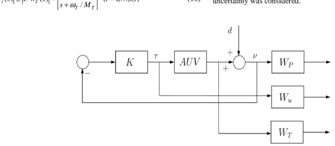
Figure 6. Augmented control system. The input signal d stands for arbitrary external disturbance.
Table 1. Summary of some design results for the AUV µ-control system.
The obtained controllers K were stable, minimum-phase, and
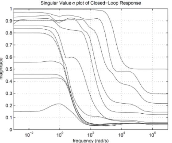
achieved robust performance. Table 1 summarizes the number of iterations and controller order based on the design performance specification of Fig. 6. Figures 7 display the obtained closed-loop
) ( ω
σ j and µ(jω) plots. Observe that these plots are in accord with peak values found in Table 1.
Design schemes with other performance specifications were tested, such as those with reference command and signal measurement noise specifications. However, because tuning of the performance weights functions requires some time and many design iterations1, we will delay these results to a forthcoming presentation. The design procedure may result in a controller possessing prohibitive high order which renders it unsuited for practical implementations. This is certainly a major method drawback2. On completion of design iterations, we verified how much of the
1
The designer should bear in mind and evaluate the satisfactory closed-loop system performance and design effort trade-offs.
2
Since the controller order equals the sum of the augmented plant's order with that of both scaling D(jω) matrices.
controller order could be reduced while still maintaining robust performance, i.e., checking whether µ∆P (N) < 1 would still hold.
One approach to find a smaller order controller is to override the automatic pre-fitting algorithm used to compute the scaling matrices
D(jω) and manually limit their order. This process was tested with
some success, making it possible to lower the controller order from 78 to 70, for the unstable system, at the cost of minimal degraded performance. Reduced order designs are not considered here, but may overcome this issue and render smaller order designs; refer to Zhou and Doyle (1998), Skogestad and Postlethwaite (1996) and the references therein.
Simulation Results
The obtained controllers K rendered the linear closed-loop system
stable and were simulated with the linear and nonlinear AUV models. These simulations evaluate the system capacity to compensate for parametric variation during system stabilization from off-nominal velocity state values. For both controller designs, a planar current scenario with a sector uncertainty region was considered.
System Stable (Uc = −1m/s) Unstable (Uc = +1m/s) D Scaling Auto-Fit. full semi full semi
Iterations 17 18 17 18 Peak µ(jω) 0.976 0.988 1.010 1.017
Peak σ(jω) 0.990 0.992 0.994 0.991
Figure 7. Closed-loop system singular values σ and strutucture singular values µ.
The system was simulated with input reference velocity trajectories in the vicinity of the nominal velocities used in the linearization. The velocity trajectories are given by pre-filtering step inputs for each system dof. These pre-filters are first order functions of time constants approximately close to 5 s. The nominal set-point velocities were initially given by [1.0; 0.1; 0.1] m/s and [0.05; 0.05; 0.05] rad/s for linear and angular dof respectively. The angular velocity set-points were simultaneously brought to zero 30s into the simulation. A set of “perturbation” reference velocity trajectories was then applied over the velocity set-points and simultaneously to all dof 20 s later, as depicted in Fig. 8. In addition, perturbation on the magnitude of the current of 0.1 m/s was considered around a constant mean value of Uc = ±1.0 m/s from the simulation start-up.
The current profile was defined on the inertial frame system. Some simulation results are shown in Fig. 8.
Discussions and Concluding Remarks
From the results presented above it can clearly be seen that AUV stabilization for surge, sway, and heave linear velocities and roll, pitch, and yaw angular velocities was satisfactorily accomplished. Reference tracking to small velocity values was also verified for both nonlinear system models considered in the System Modeling section.
The controller design for the AUV model obtained with a Uc =
+1 m/s current must satisfy an additional lower-bound constraint imposed on the complementary sensitivity weighting functions wT(s)
cut-off frequency to counteract the presence of a pair of unstable complex poles.
Nominal performance and robust stability were also verified in addition to the obtained system robust performance. In particular, robust stability can be achieved with an uncertainty set as large as |∆| < 1.8 with the obtained controller K for the AUV stable model.
Even though not designed for reference input tracking performance, the closed-loop systems with stable and unstable nonlinear system models were simulated with a reference input profile for all three translations and rotations, as described in the section above. Notice that a 2-dof scheme was adopted to define “perturbation” velocity trajectories by using a pre-filter3 to weight step input. This significantly contributed for a smooth trajectory and, therefore, time domain characteristics indicated absence of or small overshoot and tracking errors (< 0.005 m/s and < 0.005 rad/s). Steady-state error was not observed in the closed-loop system simulation results with the linearized plant model.
3
Eric Conrado de Souza and Newton Maruyama
Figure 8. Velocity tracking results.
Once again, in the present study, we have not considered the controller order as a design constraint; a typical concern for practical implementation. In this way, one could be interested in the optimal performance, that is, in obtaining the limits of achievable performance for a specified maximum controller order. Low-order controller design techniques should be employed for this intent.
Results can still be optimized for the performance of the nonlinear system model if operated over a large range of state variables4. Specifying the performance weight functions for controller design may play a role in this regard. Thus, many design iterations may be needed to determine best performance specification and the corresponding state bounds where they are satisfactorily valid. A gain scheduling scheme would then switch between the many designed linear controllers.
A final comment relates to the high number set of parametric uncertainties for the present system model. This fact may render a conservative control system design, (Skogestad and Postlethwaite, 1996). However, due to the relative high state space dimension (dof) of the full AUV velocity model, the control system design conservativeness is difficult, if not impossible in practice, to ascertain.
In summary, this note focused attention on transforming what could be considered as external disturbance into easily modeled parametric perturbation. This was carried out by considering current and added mass dynamics as parametric dependent expressions with
4
A challenging task for general, high dof-number nonlinear dynamics and certainly a recurrent issue when using linear control methods.
an associated uncertainty. A robust linear control design was performed and results were obtained with a full order nonlinear Underwater Vehicle model.
Future implementation
The present study is far from being complete and conclusive. Results still need to be optimized for performance and many questions still remain by the above considerations. Some of these could include comparisons of the above implementation with other important uncertainty modeling schemes:
• Different current uncertainty modeling, such as the physical hydrodynamic parameter uncertainty modeling, in contrast to the above proposed parametric modeling;
• Current treated as external disturbance in a mixed unstructured/parametric scheme, etc.
Alternative design methods remain yet to be implemented to this robust control problem. One such method could intrinsically consider the computation of a reduced order controller and, therefore, to treat the limit to the order for K as a design constraint.
Acknowledgements
The authors would like to thank for the sponsoring made by the Coordenação do Aperfeiçoamento de Pessoal de Nível Superior – CAPES and the Financiadora de Estudos e Projetos – Finep through the CTPetro Program.
References
Balas, G.J., Doyle, J.C., Glover, K., Packard, A. and Smith, R., 2001, “µ-Analysis and Synthesis Toolbox: Users Guide”, 3 ed., The MathWorks Inc., 3 Apple Hill Drive, Natick, MA, 01760-2098.
Campa, G., Innocenti, M. and Nasuti, F., 1998, “Robust control of underwater vehicles: sliding mode vs. µ-synthesis”, Proceedings of the OCEANS'98 IEEE Conference, pp. 1640-1644.
Feng, Z. and Allen, R., 2004, “Reduced order H∞ control of an
autonomous underwater vehicle”, Control Engineering Practice, Vol.12, No.12, pp. 1511-1520.
Fossen, T.I., 1994, “Guidance and Control of Ocean Vehicles”, John Wiley & Sons.
Fryxell, D., Oliveira, P., Pascoal, A., Silvestre, C. and Kaminer, I., 1996, “Navigation, guidance and control of AUVs: an application to the MARIUS vehicle”, Control Engineering Practice, Vol.4, No.3, pp. 401-409.
Ishidera, H., Tsusaka, Y., Ito, Y., Oishi, T., Chiba, S. and Maki, T., 1986, “Simulation and experiment of automatic controlled ROV”, Proceedings of 5th International Offshore, Mechanical and Artic Engineering Symposium, pp. 260-267.
Kalske, S. and Happonen, K., 1991, “Motion simulation of subsea vehicles”, Proceedings of the 1st Inter-national Offshore and Polar Engineering Conference, Edinburgh, UK, pp. 74-84.
Skogestad, S. and Postlethwaite, I., 1996, “Multivariable Feedback Control: Analysis and Design”, John Wiley & Sons.
Souza, E.C., 2003, “Modeling and Control of Unmanned Underwater Vehicles”, Masters in Engineering Thesis (in Portuguese), Escola Politécnica da Universidade de São Paulo.
Souza, E.C., da Cruz, J.J. and Maruyama, N., 2004, “The LQG/LTR methodology for position control of unmanned underwater vehicles”, XV Congresso Brasileiro de Automática, Gramado, RS.