Microfounded forecasting

Ensaios Econômicos

Microfounded Forecasting

Wagner Piazza Gaglianone, João Victor Issler

Setembro de 2019

Os artigos publicados são de inteira responsabilidade de seus autores. As

opiniões neles emitidas não exprimem, necessariamente, o ponto de vista da

Fundação Getulio Vargas.

EPGE Escola Brasileira de Economia e Finanças Diretor Geral: Rubens Penha Cysne

Vice-Diretor: Aloisio Araujo

Coordenador de Regulação Institucional: Luis Henrique Bertolino Braido

Coordenadores de Graduação: Luis Henrique Bertolino Braido & André Arruda Villela Coordenadores de Pós-graduação Acadêmica: Humberto Moreira & Lucas Jóver Maestri Coordenadores do Mestrado Profissional em Economia e Finanças: Ricardo de Oliveira Cavalcanti & Joísa Campanher Dutra

Piazza Gaglianone, Wagner

Microfounded Forecasting/ Wagner Piazza Gaglianone, João Victor Issler – Rio de Janeiro : FGV,EPGE, 2019

45p. - (Ensaios Econômicos; 813) Inclui bibliografia.

Microfounded Forecasting

Wagner Piazza Gaglianone

João Victor Issler

September 27, 2019

Abstract

This paper proposes a …nancial approach to economic forecasting which can be applied to data bases of surveys of forecasts. We model the forecasting decision of an individual from …rst principles (i.e., microfounded ) and show that surveys of forecasts obey an a¢ ne factor structure with a single factor which is the conditional expectation of the target variable based on common information (public and private). This holds in a context where individuals have access to public information and also have access to private information with common and idiosyncratic components. We show that asymptotically e¢ cient forecasts of the target variable can be built using the generalized method of moments in a panel-data context, when N and T diverge or when T diverges with N …xed. In this context, the optimal forecast is a function of the consensus forecast of the survey (a cross-sectional average of survey forecasts) after appropriately …ltering out two bias terms. This links the …nancial approach of economic forecasting to the forecast-combination literature, where idiosyncratic risk of individual forecasts can be diversi…ed out. Our microfounded approach is applied to a world-class data base on surveys of expectations and the techniques advanced here fare best when compared with competitive alternatives.

Keywords: Forecast Combination, A¢ ne Model, Common Factors (Features), Big Data.

JEL Classi…cation: C14, C33, E37.

The views expressed in the paper are those of the authors and do not necessarily re‡ect those of the Banco Central do Brasil or of FGV. We are especially grateful for the comments and suggestions given by Scott Atkinson, Francis Diebold, Robert Engle, Antonio Galvão, Ra¤aella Giacomini, Alain Hecq, Bo Honoré, Fabian Krüger, Michael McCracken, Marcelo Moreira, Whitney Newey, Andrew Patton, Barbara Rossi, Rafael Santos, Allan Timmermann, Mark Watson and Jonathan Wright. We also bene…ted from comments given by the seminar and conference participants around the globe, including the NBER Sum-mer Institute on Forecasting and Empirical Methods (Boston), the Annual In‡ation Targeting Seminar of Banco Central do Brasil (Rio de Janeiro), and the Conference of the International Association of Applied Econometrics (London). Gaglianone and Issler gratefully acknowledge the support from CNPq, CAPES, FAPERJ, INCT and FGV on di¤erent grants.

y_{Research Department, Banco Central do Brasil. E-mail: [email protected]}

z_{Corresponding Author. Graduate School of Economics and Finance FGV EPGE, Getulio Vargas Foundation, Praia de}

1

Introduction

Faust and Wright (2013) argue that subjective forecasts of in‡ation seem to outperform model-based forecasts in certain dimensions, often by a wide margin. They discuss some reasons why this is the case, which points out to the choice of boundary values and the fact that professional forecasters quite often have access to econometric models and add expert judgment to these models. Along the same lines, Ang et al. (2007) argue that economists use four main methods to forecast in‡ation: time-series models of the ARIMA variety; structural models built based upon the Phillips Curve; methods using information embedded in asset prices –in particular, the term-structure of interest rates; and methods that employ survey-based measures provided by economic agents (consumers and/or professional forecasters). They …nd that true out-of-sample survey forecasts (e.g. Michigan or Livingston) outperform a large number of out-of-sample single-equation and multivariate time-series competitors.

The objective of this paper is to propose a …nancial approach to economic forecasting suitable for surveys of forecasts, which have become increasingly popular as a source of forecasting methods after the work of Ang et al. and Faust and Wright. The approach is based on …rst principles, where we take seriously the optimization problem that survey respondents face in posting forecasts on a given data base.

We assume that the minimized loss function is of unknown form, heterogeneous across agents, and that agents condition on heterogeneous information as well. We also assume that the forecasting agent has no knowledge of the data generating process (DGP) of the target variable of the survey, but relies on the location-scale family of distributions that encompasses several distributions used in practice: the Normal, Uniform, Student-t, Logistic, etc. In this context, we show that optimal forecasts obey a factor model with an a¢ ne structure, mimicking canonical models in …nance. This allows employing this setup as a basis to forecast economic series combining the point forecasts contained in the survey. As far as we know, this is the …rst paper to propose such a holistic approach connecting optimal forecasts and …nancial models.

Our setup deals with heterogeneous information sets consisting of public and private information used by forecasting agents. Public information is known to all agents and pri-vate information contains common and idiosyncratic components. Optimal point forecasts obey an a¢ ne model where its common factor is the conditional expectation of the target variable based on the common information set –public and common private. Intuitively, the fact that all survey respondents are asked to forecast the same random variable nat-urally works in favor of the existence of a factor structure. But, this is not su¢ cient to guarantee it. Indeed, existence of a common factor must also rely on the fact that agents condition on common information. We give concrete examples of why this is plausible in

the context of surveys of forecasts.

Using standard econometric techniques based on the generalized method of moments (GMM), we show how one can identify and estimate the common factor, i.e., the condi-tional expectation based on public and on common private information. An alternative identi…cation and estimation method based on principal-component analysis is also feasi-ble. Using a quadratic loss in a pseudo-out-of-sample forecasting exercise, our estimate of the common component performs best when compared with commonly used alternatives. The motivation to propose a …nancial approach to economic forecasting is not new. The main idea behind forecast combinations is that, if the number of forecasts is large enough, an appropriate combination of these forecasts will eliminate idiosyncratic fore-cast errors, thereby reducing the uncertainty in forefore-casting. In 2006, Timmermann coined the phrase “a …nancial approach to economic forecasting” based on the idea of forecast combination originally proposed by Bates and Granger (1969): “A simple portfolio diver-si…cation argument motivates the idea of combining forecasts, c.f., Bates and Granger.” Several authors have worked on what could be labelled now as a …nancial approach to economic forecasting, e.g., Granger and Ramanathan (1984), Palm and Zellner (1992), Stock and Watson (1999, 2002a and b), Elliott and Timmermann (2004), Capistrán and Timmermann (2009), Issler and Lima (2009), Gaglianone and Lima (2012, 2014), Hsiao and Wan (2014), and Lahiri, Peng, and Sheng (2015).

To employ survey-of-expectation data in our setup, we propose two layers of decision making. In the …rst layer, we ask what is the optimal survey response from the point-of-view of a given respondent and what is the proper environment they generate this forecast? It is an environment where observers do not know which (heterogeneous) loss function is being optimized by each agent and where agents have no knowledge of the DGP of the target variable. We assume that survey respondents employ a potentially di¤erent location-scale model to approximate the unknown DGP, all conditioning on di¤erent covariates (heterogeneous information). Despite all these potential di¤erences for forecasters, the existence of a common-factor model for the survey of forecasts still holds: every forecaster is forecasting the same random variable in the survey and the information used by di¤erent agents usually have a common component. The latter holds even when all of them employ di¤erent covariates in their respective location-scale models, as long as these variables share a common factor as in Stock and Watson (2002b) or as in Forni et al. (2000)1_.

In the second layer of decision making, the …nal user of these economic forecasts – the econometrician – observes several forecasts posted by economic agents, indexed by i = 1; 2; ; N, across time, indexed by t = 1; 2; ; T. The econometrician has the knowledge that there exists a common-factor structure that holds for this panel data

1_{Stock and Watson’s model has a slight advantage …tting our setup since it is based on a static version}

base. If the econometrician employs a mean-squared-error (MSE) risk function, which is typically the case for the government, a central bank, a large risk-neutral …rm, etc., it will be optimal for her/him to extract from the survey of expectations its common factor –the conditional expectation of the target variable given a common information set2. We show how to estimate consistently this conditional expectation by employing a GMM approach. This estimate is a combination of forecasts –a bias-corrected combination of forecasts.

The techniques discussed above are appropriate to be applied to current surveys of economic forecasts, which are panels characterized by a limited number of respondents (limited N ) and a large and increasing number of time-series observations (large T ), e.g., The Survey of Professional Forecasters, The Michigan Survey, The Livingston Survey, The Bloomberg Survey of Economists, etc. In a world where there is an increasing availability of reliable data provided electronically, it is interesting to examine how one could e¢ ciently use this wealth of information, since, in the future, we will be dealing more and more with big data surveys – very large N and T . Indeed, the techniques proposed in this paper also apply to future big data surveys as well. This is important since as Einav and Levin (2014) have put it: “The most common uses of “big data” by companies are for tracking business processes and outcomes, and for building a wide array of predictive models”.

The ideas in this paper are related to research done in three di¤erent …elds. From econometrics, it is related to the common factor literature after Geweke (1977) and Sar-gent and Sims (1977), perhaps best represented by the work of Forni et al. (2000) and Stock and Watson (2002b), and the common features literature after Engle and Kozicki (1993). Regarding the latter, we attempt to bridge the gap between a large literature on common features applied to macroeconomics, e.g., Vahid and Engle (1993, 1997), Engle and Issler (1995), Issler and Vahid (2001, 2006) Vahid and Issler (2002), Hecq et al. (2006), Athanasopoulos et al. (2011), and the econometrics literature on forecasting related either to common factors or to forecast combination, perhaps best represented by the work of Bates and Granger (1969), Granger and Ramanathan (1984), Palm and Zellner (1992), Davies and Lahiri (1995), Forni et al. (2000, 2005), Stock and Watson (2002a,b, 2006), Elliott and Timmermann (2004, 2005), Timmermann (2006), Patton and Timmermann (2007), Issler and Lima (2009), Atak, Linton and Xiao (2011), Gaglianone et al. (2011), Gaglianone and Lima (2012, 2014), and Lahiri, Peng, and Sheng (2015). In this context, it is also related to the literature on the role of loss functions, e.g., Elliott et al. (2008) and Capistrán and Timmermann (2009). From big data econometrics it is related to the work of Diebold (2012), Einav and Levin (2014), and Varian (2014).

The techniques proposed here are applied to a world-class data base on in‡ation ex-pectations – The Focus Survey of forecasts – a unique panel data base put together by

2_{Of course, di¤erent risk functions in the second layer would imply extracting a di¤erent target. This}

the Brazilian Central Bank (BCB). It collects daily expectations from professional fore-casters in commercial banks, asset management …rms, consulting …rms and non-…nancial institutions, followed throughout time with a reasonable turnover. It contains a set of 298 registered institutions in the system, with a smaller active group of around 100 in-stitutions. Our sample covers daily in‡ation forecasts of monthly IPCA in‡ation from January, 2nd, 2006, to June 7th, 2018 (3; 165 working days). The forecast horizon ranges from one day up to 400 days, forming a three-dimensional unbalanced panel containing a total amount of 4; 712; 424 observations. Under MSE risk, our estimate of the common factor (feature) of in‡ation expectations fares better than frequently employed forecast-combination techniques, the best ARMA model chosen using Schwarz Criterion, as well as principal-component based techniques. When we compare our method with alterna-tive forecast-combination techniques, MSE reductions can reach up to 10%. Reductions vis-à-vis the MSE associated with forecasts of the best ARMA model can reach up to 49%. The rest of the paper is divided as follows. Section 2 introduces a microfounded-based framework to study the forecast error under risk functions more general than the usual MSE. Section 3 presents a real-time forecasting exercise with data from The Focus Survey of Brazilian in‡ation expectations, comparing the out-of-sample performance of di¤erent forecasting approaches. Section 4 concludes.

2

Microfounded forecasting under a general risk

func-tion

The techniques discussed in this section are appropriate for forecasting a strictly stationary and ergodic univariate process fytg, with …nite …rst and second moments, using a large number of forecasts. Covariates used in forecasting are also strictly stationary and ergodic with …nite …rst and second moments. We restrict these forecasts to be the result of a survey on the target variable yt. We can also imagine that some (or all) of these responses are generated using econometric models, but then the econometrician that observes these forecasts has no knowledge of them.

We label individual forecasts of yt, computed using information sets lagged h periods, by fi;th, i = 1; 2; : : : ; N , and t = 1; 2; : : : ; T . Therefore, fi;th are h-step-ahead forecasts of yt, formed at period t h; and N is the number of respondents of this survey of expectations regarding yt.

In this paper, we show that, optimal forecasts obey a factor model with a single factor Et h(yt) – the conditional expectation of yt computed using a common information set

lagged h periods3_:

f_i;th = k_ih+ h_iEt h(yt) + "hi;t; (1) where kh

i, h

i and "hi;t, represent, respectively, a heterogeneous intercept bias-correction term, a heterogeneous slope bias-correction term, and an idiosyncratic error term.

The core idea

Before formalizing the assumptions needed to derive our main results, we believe the reader will bene…t from a basic explanation of what this paper is about. Consider the setup in Patton and Timmermann (2007), where each individual i chooses the optimal point forecast fi;th so that the conditional expected loss function (Li) is minimized:

f_i;th = arg min fi

E Li(yt; fi)jFi;t h : (2)

Here, fi 2 R represent all possible point-forecast choices for forecaster i; the conditioning information set Fi;t hvaries across forecasters (heterogeneous information) and is based on both public and private information; there is an unknown risk function used by forecaster i (loss-function heterogeneity), and an unknown conditional DGP of yt used by the agent to compute E [Li_(y

t; fi)jFi;t h] and therefore to forecast yt.

We assume that the optimizing agent i employs the location-scale model with one covariate alone4_{, di¤erent for every agent, where the conditional quantile function of y}

t, Qyt( jFi;t h), reads as:

Qyt( jFi;t h) =

h

0;i( ) + h

1;i( ) xi;t h; (3)

where xi;t h is the covariate used by agent i in the location-scale model, 2 [0; 1] is a quantile of the conditional distribution of yt, and h0;i( ) and h1;i( ) are parameters that vary across quantiles ( ), agents (i), and forecast horizons (h), but do not vary across time to preserve stationarity. To simplify notation here, we drop the dependence of h

0;i( ) and h

1;i( ) on h in what follows.

We must stress that we assume an extreme case that works against common informa-tion, since each agent employs a di¤erent covariate xi;t h in their respective location-scale model (heterogeneity in information). Despite that, these covariates, xi;t h, should be correlated with each other, since they are all used to model and forecast the same random variable yt and therefore must all have some predictive power for yt5. One well-known

3_{Indeed, (1) is an encompassing model. Some results we derive in the Appendix, as well as in the}

Online Technical Appendix, represent restrictions on this general formula.

4_{The generalization for a multi-covariate setup is discussed in the Online Technical Appendix.}

model in the forecasting literature which delivers correlated regressors is Stock and Wat-son’s (2002b) factor model. In our context, it reads:

yt = 0FFt h+ 0wwt h+ t;

xt = Ft+ et; (4)

where xt= (x1;t; x2;t; ; xN;t)0 stacks all the covariates used by the agents to forecast yt; Ftstacks a reduced number of r (r N )latent factors capturing the common components of these covariates and generating their cross-correlation; wt stacks additional regressors used to forecast yt, e.g., its lags; and tand etare errors terms which are allowed to be both serially correlated and (weakly) cross-sectionally correlated. In what follows we assume that either (4) holds or that a similar factor structure holds to assure that the covariates have a common component.

An important result from Patton and Timmermann (2007) regarding an optimal point forecast fh

i;t is that it is associated with a given quantile level of Qyt( jFi;t h), labelled

here as _i, which may di¤er across i, as follows:

f_i;th = Qyt( i jFi;t h) = F_{i;tjt h}1 ( i) : (5) In words, the point forecast fh

i;tis a speci…c conditional quantile of yt, where Fi;tjt h( )is the conditional cumulative distribution function of yt. The key here is that each point forecast lies in the domain of the conditional cumulative distribution, so that the conditional probability of yt fi;th could be computed and Fi;tjt h ( ) inverted. Given (3), we can apply this result to (5) to obtain:

f_i;th = Qyt( i jFi;t h) = 0;i( i) + 1;i( i) xi;t h: (6) Notice that this establishes an a¢ ne relationship between the covariate in the location-scale model and the optimal individual forecast. However, for every respondent, we can go one step further to relate the latter with the conditional mean of yt, E (ytjFi;t h) Ei;t h(yt), given all the information available to the agent. This could be accomplished by using another important result (Koenker, 2005), which relates the conditional quantile

function with the conditional mean Ei;t h(yt): Z 1

0

Qyt( jFi;t h) d = Ei;t h(yt), or,

Ei;t h(yt) = Z 1

0

[ 0;i( ) + 1;i( ) xi;t h] d = Z 1 0 0;i( ) d + xi;t h Z 1 0 1;i( ) d , or,

= 0;i+ 1;ixi;t h; (7)

where 0;i = R1

0 0;i( ) d and 1;i = R1

0 1;i( ) d . Combining (6) and (7), we arrive at:

f_i;th = 0;i( i) 1;i( i) 0;i 1;i + 1;i( i) 1;i E i;t h(yt); (8) which establishes an a¢ ne relationship between the optimal individual forecast and the individual conditional expectation Ei;t h(yt) of agent i.

We now turn to the components of the individual information sets used by every agent. The information set Fi;t h is partitioned into three mutually orthogonal (and non-empty) components: Ft h, Ft hP C, and Fi;t hP I , where Fi;t h = Ft h[ Ft hP C [ Fi;t hP I . The public information set, denoted by Ft h, is the information set available to all forecasters. Private information is in turn decomposed into the private-common information set FP C

t h (e.g., paid-up news and forecasts used by agents in the market, paid macroeconomic reports, etc.) and the private-idiosyncratic information set Fi;t hP I (e.g., idiosyncratic private information (paid-up or not), individual expert judgement, etc.).

One important result widely used in the Nowcasting literature, e.g., Ba´nbura, Gian-none, and Reichlin (2011), is the orthogonal-component decomposition6_:

Ei;t h(yt) E (ytj Fi;t h) = E (ytj Ft h) + E ytj Ft hP C + E ytj Fi;t hP I ; (9)

where it becomes clear that heterogeneity appears only in the last term of (9), while Et h(yt) E (ytj Ft h) + E yt j Ft hP C contains the common part of expectations for all

6_{A simple example of this decomposition relates to the linear regression model:}

y = X + "; where the OLS estimator decomposes y as:

y = X b +b"

= X (X0X) 1X0y +hI X (X0X) 1X0iy;

the …rst term being a projection onto the space of X and the second being a projection onto the orthogonal space of X.

agents i = 1; :::; N . Combining (8) and (9), we arrive at: f_i;th = 0;i( i) 1;i( i) 0;i 1;i + 1;i( i) 1;i E t h(yt) + 1;i( i) 1;i E y tj Fi;t hP I = 1;i( i) 1;i E (y t) + 0;i( i) 1;i( i) 0;i 1;i + 1;i( i) 1;i E t h(yt) + 1;i( i) 1;i E y tj Fi;t hP I E (yt) = 1;i( i) 1;i E (y t) + 0;i( i) 1;i( i) 0;i 1;i + 1;i( i) 1;i E t h(yt) + "hi;t; (10) where "h i;t = 1;i( i) 1;i E ytj F P I

i;t h E (yt) is the conveniently demeaned idiosyncratic component of individual expectations.

As promised, equation (10) delivers an a¢ ne factor model with a single factor related to common information sets among forecasters in the survey. We can use (10) to check well known results in the literature. Suppose that the loss function being used by individual i is quadratic. Then, her/his optimal forecast is the conditional mean:

f_i;th _{= E}t h(yt) + E ytj Fi;t hP I = Ei;t h(yt); (11)

which is the result obtained from (10) since the optimal alphas will be their respective means in this case, i.e., 0;i( i) = 0;i and 1;i( i) = 1;i. Additionally, if the conditional density function of ytis symmetric, then, for agent i, 1;i( i) = 1;i(1=2) = 1;i, 0;i( i) =

0;i(1=2) = 0;i. Using these results in (10) gives:

f_i;th _{= E}t h(yt) + E ytj Fi;t hP I = Ei;t h(yt) = Mediani;t h(yt) : (12)

Now we interpret our key result here. First, the two examples in (11) and (12) illustrate that asymmetry of the loss function is responsible for the intercept and slope terms in (10), therefore, this is the basis for the a¢ ne structure. Second, the fact that we have obtained a factor model with a single common factor is not surprising, since all surveys respondents are asked to forecast the same random variable yt. Intuitively, some commonality is expected to be present. However, in our extreme case, all agents employ a di¤erent covariate in forecasting. The common-component survives at the end because all survey respondents forecast the same random variable and because their information sets have common components, as (4) makes explicit, despite the fact that all covariates are di¤erent. Third, in a context where it only exists public information, the optimal forecast under MSE risk in the second layer will be E (ytj Ft h). In the presence of private information as well, if all the econometrician observes is public information, but not the (common) private information observed by individual agents, then, the common factor will actually give a

bonus to the econometrician: the optimal forecasts in the second layer of decision making would still be E (ytj Ft h), but the common factor will deliver Et h(yt) = E (ytj Ft h) + E ytj Ft hP C , which will have a superior forecasting performance, since the conditioning set was expanded. Third, in the more realistic case where the econometrician has access to public and common-private information, then her/his optimal forecasts in the second layer will be Et h(yt) = E (ytj Ft h) + E ytj Ft hP C , exactly the common factor of the survey of forecasts.

Identi…cation and GMM estimation

The optimal forecasts fh

i;t took the encompassing general form:

f_i;th = k_ih+ h_iEt h(yt) + "hi;t; (13)

where a full mapping from (10) to (13) is straightforward to obtain:

k_ih = 1;i( i) 1;i E (y t) + 0;i( i) 1;i( i) 0;i 1;i ; h i = 1;i( i) 1;i ; "h_i;t = 1;i( i) 1;i E y tj Fi;t hP I E (yt) :

Now consider an econometrician who operates under MSE risk and only observes a survey of individual forecasts fh

i;t (all optimal, in principle) and the target variable yt. Given the existence of (13), she/he could rely on the a¢ ne structural model to estimate (or extract) the latent factor Et h(yt)from survey data. The survey is a three-dimensional panel, with t = 1; :::; T , i = 1; :::; N , and h = 1; :::; H. Although the horizon can in principle increase without bound, when forecasting one usually keeps H small, since in a stationary-ergodic world, as H increases, conditional forecasts converge to their uncondi-tional counterparts, making the case for large H unappealing.

As argued before, our framework entails two interesting cases. The …rst is T ! 1, with small N and H, which applies to some long standing surveys with an almost constant number of respondents throughout time. The second is T ! 1, N ! 1, and small H, which applies to large surveys taken across a long period of time. At the time of writing, we see no surveys of expectations that could …t this pro…le. But, this does not mean that we should ignore it. In a world where there is an increasing availability of reliable data provided electronically, it is interesting to examine how one could e¢ ciently use this wealth of information for forecasting. There is already a large literature on big data in statistics, but it could bene…t from economic interpretation o¤ered by the (quasi-structural) factor

model discussed above. In the future, surveys of expectations would include the abundant information on thousands or millions of respondents on an almost continuous-time basis. This makes the big data setup where T ! 1, N ! 1, and small H, of interest to be applied in the Surveys of the Future, being the reason why we discuss them here.

There is one hurdle to overcome when N and T are large –the curse of dimensionality when N ! 1. Even when H is small, the system of equations (13) has too many parameters that grow without bound. This poses a problem for the identi…cation of Et h(yt). One key issue is that we do not need the identi…cation of all kih and

h i, i = 1; :::; N_{, to be able to identify E}t h(yt). Indeed, under suitable conditions, we only need to know their respective means.

Our basic proposed approach to identify and estimate Et h(yt) is to employ the gen-eralized method of moments (GMM), relying on T asymptotics. However, the fact that Et h(yt) is a latent variable is a drawback, since the moments used in GMM estimation must be a function of observables and parameters alone. However, one can always decom-pose the series ytinto Et h(yt)and an unforecastable martingale-di¤erence component ht, such that Et h( ht) = 0:

yt = Et h(yt) ht: (14)

Combining (13) and (14) leads to:

f_i;th = k_ih+ h_i(yt+ ht) + " h i;t (15) = k_ih+ h_iyt+ vhi;t; (16) where vh i;t h

i ht+"hi;t is a composite error term. Notice that, by construction, Et h ht = 0_{, so E}t h vhi;t = 0if one assumes that Et h("hi;t) = 0. Starting with (16) and Et h vhi;t = 0, and using the law of iterated expectations and valid observable instruments zt s, where s h, we obtain: E fi;th k h i h iyt zt s = 0; (17)

which is valid for all i = 1; :::; N , t = 1; :::; T , and h = 1; :::; H. The system (17) has 2N H parameters and (at least) 2N H moment conditions, provided that dim(zt s) > 2, which is critical for over-identi…cation. Despite that, one problem remains: as N ! 1, the amount of parameters in (17) diverges, which goes against consistency.

To eliminate the curse of dimensionality problem, we take the cross-sectional averages of terms fi;th kih

h

iyt, leading to the following moment restrictions: Eh fh

;t kh hyt zt s i

t = 1; :::; T, and h = 1; :::; H, where fh ;t = N1 N X i=1 f_i;th, kh ₌ 1 N N X i=1 kh_i and h = _N1 N X i=1 h i, represent cross-sectional averages for each h.

Therefore, the system in (18) can be the basis to estimate kh _and h _{consistently in a} context where T ! 1, with small N and H.7 _{It is straightforward to show identi…cation} of Et h(yt)using the conditional version of (18):

Et h h fh ;t kh hyt zt s i = 0: (19)

For every instrument in zt s, say, zj;t s, j = 1; 2; ; k, where k > 2, we can solve (19) to obtain: 0 k 1= Et h 2 6 6 6 6 6 6 4 0 B B B B B B @ fh ;t kh h yt z1;t s fh ;t kh h yt z2;t s .. . fh ;t kh h_y t zk;t s 1 C C C C C C A 3 7 7 7 7 7 7 5 = 2 6 6 6 6 6 6 4 0 B B B B B B @ fh ;t kh h Et h(yt) z1;t s fh ;t kh h Et h(yt) z2;t s .. . fh ;t kh h Et h(yt) zk;t s 1 C C C C C C A 3 7 7 7 7 7 7 5 : (20) since the average forecast, fh

;t, and all the instruments zj;t s, j = 1; 2; ; k, are observable regarding the information set Ft h[ Ft hP C. If we divide every equation in the system (20) by its respective instrument, and then solve them all for Et h(yt), we obtain the same result: Et h(yt) = fh ;t kh h = 1 N N X i=1 fh i;t kh h :

Hence, as long as we can estimate kh _and h _{consistently by GMM, we can identify} Et h(yt), relying on T -asymptotics.

Once one deals successfully with consistency, one can start worrying about e¢ ciency in a GMM context. One way to exploit all possible moment conditions implicit in (18) is to stack all the restrictions across h (…nite) as:

E 2 6 6 6 6 6 4 0 B B B B B @ f1 ;t k1 1_y t f2 ;t k2 2 yt .. . fH ;t kH H yt 1 C C C C C A zt s 3 7 7 7 7 7 5 = 0; (21)

where our problem collapses to one where we have H dim(zt s) restrictions and 2H parameters to estimate. As before, over-identi…cation requires that dim(zt s) > 2. Given a choice of H, GMM estimation of (21) is e¢ cient. A less e¢ cient alternative to estimate

7

the whole stacked system (21) is to estimate separately (18) for every horizon h, which could also be attempted for computational reasons.

In the context of N; T ! 1, with H small, we now discuss the case where we …rst let N ! 1 and then let T ! 1, using the sequential asymptotic framework of Phillips and Moon (1999). Under suitable conditions, the cross-sectional averages in (18) and (21) would converge in probability to a unique …nite limit as N ! 1, i.e., _{1 < plimN}1 N X i=1 h i = h _< 1, 1 < plimN1 N X i=1 kh i = kh < 1, and 1 < plim_N1 N X i=1

f_i;th = fh_;t < _{1, for all t = 1; 2; : : : ; T . Then, a key condition for T -consistent} estimation is that (18) and (21), evaluated at these limits are a unique solution for each of them respectively. Take now moments (18), considering that N ! 1:

E fh;t kh h yt zt s = 0; or, (22) E h ht zt s = 0; (23) under _N1 N X i=1 "h i;t p

! 0, as N ! 1, t = 1; :::; T , and h = 1; :::; H. Note that (23) is attained by construction, since h

t is a martingale-di¤erence and must be orthogonal to all series dated t hor before. In this context, GMM provides a consistent estimate for parameter means as T ! 1.

To prove it, …rst de…ne h = [kh_; h_{]0 and consider the following assumptions –(A1-A3)} – all laid out in the Appendix A. Assumption A1 guarantees that the errors "h

i;t can be diversi…ed away, and that cross-sectional dependence is not a problem. By its nature, "hi;t is a function of expectations based upon idiosyncratic information, therefore diversi…able. Assumption A2 just requires …nite convergence of di¤erent cross-sectional averages, which bounds the degree of cross-sectional and time-series dependence due to spatial dependence. Assumption A3 deals with GMM identi…cation and is standard in the literature. We can now state an important result, which allows for consistent estimation of Et h(yt).

Proposition 1 Under assumptions A1-A3, the Extended BCAF (Bias Corrected Aver-age Forecast) 1 N N X i=1 f_i;th kch

ch , based on T -consistent GMM estimates b

h = h b kh_{; c}hi0_{; obeys} plim (N;T !1)seq 1 N N X i=1 fh i;t kch ch !

= Et h(yt) = E (yt j Ft h)+E ytj Ft hP C , where (N; T ! 1)seq denotes the sequential asymptotic approach proposed by Phillips and Moon (1999), when we let …rst N ! 1, and then let T ! 1.

In the context of N; T ! 1, an alternative to GMM estimation is to employ the principal-component analysis proposed in the common factor literature in economics and

…nance based on the results of Forni et al. (2000) and Stock and Watson (2002b). There, consistent estimation of the common factor requires both N and T to diverge without bound. Therefore, they …t perfectly well the setup of what we have called the Surveys of the Future, where N; T ! 1. However, they do …t exactly the setup of current surveys of expectations, where T ! 1 but N is …xed. In this case, GMM estimation has the advantage of relying on T asymptotics alone to estimate kh _and h_{, regardless of whether} N _{! 1 or not. In the empirical section, we compare the forecasting accuracy of GMM} based estimates of Et h(yt)with that of principal-component based estimates.

We now turn to the case where we let T ! 1 with N …xed, or to the case of sequential asymptotics where we let …rst T ! 1, and then N ! 1. The critical issue of letting T _{! 1 …rst is that, when we take cross-sectional averages as in (18) or (21), but N is not} large, we have to guarantee that for all possible ensemble averages Et h(yt) is identi…ed. When we assume the opposite sequential order, we have only to worry about identi…cation of a single limit case. An added complication for N small is that 1

N N X

i=1 "h

i;t does not vanish in probability. Recall that A3 imposes that E "hi;t = 0 for all i and t, given h. This is not su¢ cient to guarantee that moments (18) and (21) can be cast in terms of h

t alone. However, employing the assumption that Et h("hi;t) = 0 is su¢ cient to validate (18) and (21). Thus, we employ two assumptions (A4-A5) laid out in the Appendix A.

Proposition 2 Under assumptions A4-A5, the Extended BCAF (Bias Corrected Aver-age Forecast) _N1 N X i=1 fh i;t kch

ch , based on T -consistent GMM estimates

bh _{= k}bh_;ch 0 , obeys plim T !1 1 N N X i=1 fh i;t kch ch !

= Et h(yt) = E (ytj Ft h)+E ytj Ft hP C , where we let T ! 1, with N _{…xed. The convergence to E}t h(yt) also happens when we let …rst T ! 1 and then let N ! 1, that is, plim

(T;N !1)seq 1 N N X i=1 f_i;th kch ch ! = Et h(yt) = E (ytj Ft h) + E ytj Ft hP C , where (T; N ! 1)seq denotes the sequential asymptotic approach proposed by Phillips and Moon (1999).

Notice that assumptions A4 and A5 su¢ ce to provide T -consistent GMM estimates for all bounded N . Indeed, …xed N is a special case of (T; N ! 1)seq, where we do not let N diverge after T ! 1, the context being identical otherwise. For the sake of completeness, it is interesting to cover the case of joint convergence, where we can establish a link between sequential convergence and joint convergence following Phillips and Moon (1999). However, to save space in the main text, this is done in section 2 of the Online Technical Appendix of this paper.

Decomposing information

Once we have a consistent estimate of:

Et h(yt) = E (yt j Ft h) + E ytj Ft hP C ;

we can estimate a mixed-e¤ect panel-data model (also known as the mixed linear model) that takes into account individual heterogeneity in regression coe¢ cients; see Cameron and Trivedi (2009) for a basic introduction in a panel-data context and Searle, Casella, and McCulloch (1992) and McCulloch, Searle, and Neuhaus (2008) for a more general treatment:

f_i;th = kh_i + h_iEt h(yt) + "hi;t; where (24) k_ih = kh₀ + _i; _{i N 0;} 2 ;

h i =

h

0 + i; i N 0; 2 :

Following the mixed-e¤ect panel-data literature, we estimate (24) by maximum likeli-hood assuming a random-e¤ect speci…cation for i and i. This allows the identi…cation of the demeaned idiosyncratic component "h

i;t = h

i E ytj Fi;t hP I E (yt) , whose estimate will be the regression residual. Indeed, we can solve for E ytj Fi;t hP I as:

E ytj Fi;t hP I = 1

h i

"h_{i;t+ E (y}t) ;

therefore being able to identify E yt j Fi;t hP I given a consistent estimate for "hi;t, h i, and E (yt). Since Propositions 1 and 2 o¤er a consistent estimate of

Et h(yt) = E (yt j Ft h) + E ytj Ft hP C ; (25)

we can identify:

Ei;t h(yt) = Et h(yt) + E yt j Fi;t hP I ; (26) and decompose individual conditional expectations into two distinct terms: a common component and an idiosyncratic component.

In our context, the common component in (25) is based on public and private infor-mation. But, the key di¤erence between them is that the former is freely available for all agents whereas the latter has to be paid for, despite being common. The fact that the pri-vate common information is available to every agent gives it a public ‡avor. Therefore, we can regard (26) as decomposition of individual expectations into a “public” and a private component, which are orthogonal.

the social value of public information as examined by Morris and Shin (2002). The way they label information is as follows: “to the extent that one decision maker’s choice is made in isolation from others, more information is generally bene…cial. This conclusion is una¤ected by whether the incremental information is public (shared by everyone) or private (available only to the relevant individual).”So the de…nition of public and private hinges solely upon whether it is shared by everyone or it is only available to an individual, matching exactly our de…nitions of common and idiosyncratic, respectively.

As Shiller (2000) puts it, “signi…cant market events generally occur only if there is similar thinking among large groups of people,” which occurs if the importance of the common (public) component is high. The decomposition in (26) allows measuring the relative importance of its two terms. Since they are orthogonal:

1 = VAR [Et h(yt)] VAR [Ei;t h(yt)] +VAR E ytj F P I i;t h VAR [Ei;t h(yt)] , (27)

will give the relative importance of Et h(yt) and E yt j Fi;t hP I in (26) across time and agents.

Discussion

The optimal forecasts in Propositions 1 and 2 are a function of the consensus forecast of the survey (a cross-sectional average of survey forecasts) after appropriately …ltering out two bias terms, therefore being a forecast-combination approach. This links the …nancial approach to economic forecasting to the forecast-combination literature. Indeed, if the number of forecasts is large enough, i.e., N ! 1, all idiosyncratic forecast risks are diversi…ed away, since _N1

N X

i=1

"h_{i;t ! 0. Indeed, this is a basic principle behind large portfolio}p analysis.

The GMM approach in Propositions 1 and 2 works under N; T ! 1, but it also works with T ! 1 and N …xed. Alternative identi…cation strategies could be pursued, especially those that are based on principal-component analysis, e.g., Stock and Watson (2002b). Indeed, we also employ these techniques to estimate the optimal forecast in the second layer and compare results with our GMM approach. As noted above, the principal-component approach requires N; T ! 1. This is an extreme assumption in view of the fact that current surveys of expectations have a limited number of respondents, i.e., N < 1. Therefore, current data does not …t the asymptotic assumptions in this literature.

Another possibility is to employ a within-group method proposed by Bai (2009). This allows for the joint presence of additive and interactive e¤ects. In our notation, Bai’s

structure would be: f_i;th = Xi;t + + kih+ h t + h iEt h(yt) + "hi;t: (28) One could think that our a¢ ne structure could be viewed as a special case of Bai’s model, where Xi;t = 0 and = 0. However, identi…cation of Bai’s latent factor (Et h(yt) here) requires constraining PN_i=1 h_i = 0 and PT_t=1Et h(yt) = 0, which our method avoids.

One important character of our method is that it extends the previous literature on a …nancial approach to economic forecasting using panel data, e.g., Palm and Zellner (1992), Davies and Lahiri (1995), Davies (2006), Issler and Lima (2009), Gaglianone and Lima (2014), and Lahiri, Peng, and Sheng (2015). For example, our setup encompasses that of Davies and Lahiri (and Davies), reproduced below with our notation:

yt fi;th = kih+ ht + "hi;t ; (29)

since they impose h_i = 1 for all i = 1; :::; N and all h = 1; :::; H. Also, we generalize the results in Issler and Lima, who use h_i = 1 for all i = 1; :::; N in (13), since they have only one source of bias correction –the intercept.

Finally, our factor model has an important contribution to rationality tests in fore-casting, after Mincer and Zarnowitz (1969). For a given horizon h, we have proposed to estimate the parameters in fh

;t kh hyt, i.e., (18), by using instrumental-variable (IV) techniques. In the GMM approach, the regression of interest is fh

;t kh hyt whereas the elements in zt s are valid instruments. Here, the IV regression estimates the aver-age intercept and slope biases, respectively, kh _and h_{, and we can think that f}h

;t is the dependent variable and yt and a constant term are the regressors.

In contrast, the aggregate version of the Mincer and Zarnowitz (1969) approach starts from an inverse regression relating yt to fh;t, and tests for no bias involving zero intercept and unit slope, i.e., it uses:

fh

;t = kh+ h

yt+ vh;t, to get the inverse regression, (30) yt = kh h + 1 hf h ;t vh ;t h; (31)

where (31) is the usual aggregate Mincer-Zarnowitz regression. The standard procedure is to estimate kh_h and 1_h by least squares, which is then used to test for an unbiased consensus: a joint test of kh _{= 0 and} h _{= 1; see the discussion in Gaglianone, Issler} and Matos (2017). What is striking here is that, in the presence of the factor model (16), one cannot estimate (31) by least squares, since the regressor fh

;t is correlated with the error term v

h ;t

something the literature on Mincer-Zarnowitz testing misses.

3

Empirical Application

Data

The Focus Survey of forecasts is a world-class panel database put together by the Brazilian Central Bank (BCB), which collects daily information from professional forecasters of commercial banks, asset management …rms, consulting …rms and non-…nancial institutions, followed throughout time with a reasonable turnover. As new participants are often added to the survey, and others drop out, the panel of survey forecasts is unbalanced. From a set of 298 registered institutions in the system, there is a smaller active group of around 100 institutions that frequently update their nowcasts and forecasts. These are supplied over di¤erent forecast horizons and for a large array of macroeconomic time series; see Marques (2013).

Our target variable is Brazilian in‡ation, as measured by the Broad National Consumer Price Index (IPCA), collected at the monthly frequency. IPCA in‡ation is a key variable for the Brazilian In‡ation-Targeting Regime, since it is the o¢ cial in‡ation-target variable. If the number of survey respondents were very large, this could potentially serve to approximate a large N; T environment, since our data covers forecasts collected every working day from the period of January 2nd, 2006, to June 07th, 2018 (3; 165 working days)8_{. However, since we must rely (with respect to nowcasts) on the active group of} about 100 institutions to comprise the cross-section, the framework here is that of a large T _{with …xed N , or, at best, one in which we let …rst T ! 1, and then let N ! 1.}

In every working day considered within our sample, market agents, i = 1; :::; N , may in-form their expectations regarding in‡ation rates all the way up to the next 14 months. The raw data contains forecasts for "…xed-events" and varying forecast horizons; see Bakhshi et al. (2005). To …t the setup discussed in (18) and (21), the original forecasts are re-organized to form time-series of …xed horizons h and time-varying events (t = 1; :::; T = 150 months). As a result, the original data set formed an unbalanced panel (N T H) con-taining 4; 712; 424 observations. However, due to the transformation from …xed-event to …xed-horizon, as well as to the application of a …lter for agents that had a reduced num-ber of time-series observations, the …nal data base used in this paper contains 3; 594; 951 observations.

Decomposing our total of 3; 594; 951 observations into N , T , and H, gives the following breakdown: t = 1; :::; T = 150 months (or events), h = 1; :::; H = 400 days (or forecast

8_{The Focus Survey database has been collected since 1999, the year in which the Brazilian}

in‡ation-targeting regime was created. However, in its inception, the survey had only a small coverage (small N ), that being the reason why we start the forecasting exercise in 2006.

horizons), and an average of i = 1; :::; N = 59:92 forecasters, when considering the full term-structure of 14 monthly forecasts. We must also stress that the great majority of survey respondents provided nowcasts and/or short-term forecasts, but only a smaller set of respondents inform their forecasts for the full term-structure of forecasts, up to the longest horizon.

To implement our forecasting exercise, we split our time-series sample into two consecu-tive sub-periods: the …rst (t = 1; :::; T1)is labeled as “training sample”, where realizations of yt are usually confronted with forecasts provided by the survey, and potential bias-correction terms are estimated using either (18) or (21). We choose T1 = 60 months. The second sub-period is where genuine out-of-sample forecasts are entertained. This period comprises the last P observations of our sample (t = T1+1; :::; T )–where P = T T1 = 90 months. These P observations are thus used to compare di¤erent forecasts, computing forecast-accuracy measures.9

To evaluate a given forecast method, we compute M SEh = _P1 T P t=T1+1 yt fbth 2 , where b fh

t is the h-step ahead forecast (of yt formed at period t h) of any given method. Here, we considered …ve types of forecast methods. The …rst is the one proposed in this paper – which we have labelled the extended bias-corrected average forecast (EBCAF). The second is the simple cross-sectional average forecast – average forecast (AF) for short. It has a long tradition in econometrics, all the way from Granger (1969), to Stock and Watson (2006), and Capistrán and Timmermann (2009), among others. The third is the bias-corrected average forecast –BCAF for short. It was proposed by Issler and Lima (2009) and performs an intercept correction of the average forecast. The fourth is the Principal Component Analysis (PCA), which is a well-known data-reduction technique, applied here to summarize the information content of the cross-section of forecasts; see Stock and Watson (2002b). The last method is the AR (1) model: within the ARMA class, it is the best one-step ahead predictor of Brazilian in‡ation for our sample as a whole (T = 150 months) according to several di¤erent Information Criteria. It will be used here as our basic benchmark.

In constructing the EBCAF, we used a set of instruments containing lagged in‡ation t and interest it rates (IPCA and SELIC, respectively). Interest rates are transformed by …rst-di¤erences of logs. The results are based on the following set of instruments: zt s = [1; t s; t s 1; t s 4; ln it s 1; ln it s 4; ln it s 10]0 with s = 14 months to cover the longest horizon. In GMM estimation, the key parameters in the extended BCAF were estimated using (18) for each horizon (h), instead of using its stacked version –

9_{We use a recursive estimation scheme (i.e., increasing training sample size). In this context, each}

model is initially estimated using the …rst T1= 60 observations (excepting the average forecast method )

and the out-of-sample point forecasts of yT1+h, h = 1; :::; H, are generated. We, then, add an additional

observation at the end of the training sample, re-estimate the models and generate again out-of-sample forecasts. This process is repeated along the remaining data.

equation (21). In practice, estimation of the stacked version (21) was not feasible. The empirical exercise was conducted using the R software (version 3.2.2 i386), and the package "GMM" encoding the "two step" approach of Hansen (1982) was employed, although the "iterative" procedure of Hansen et al. (1996) yielded very similar results.

Empirical Results

Figure 1 shows the monthly CPI in‡ation (IPCA) in Brazil. In‡ation seems to conform to a stationary-ergodic process. For example, all tests for unit roots reject I (1)-ness. As noted before, within the ARMA class, in‡ation is best described by an AR (1) model with an estimated AR (1) coe¢ cient of 0:682 –estimated standard error of 0:059. Figure 2 plots monthly in‡ation and the respective daily forecast for survey respondents at horizons h = 30; 60; 180; 360 days. It also presents the AR(1) forecasts, the average forecasts, the PCA10 _{forecasts, the BCAF, and the extended BCAF, at these same horizons.}

Figure 1 - In‡ation rate (yt) in Brazil: % monthly

Table 1 reports GMM estimates for the extended BCAF. Hansen’s (1982) over-identifying restriction test (J-test) does not reject the orthogonality between errors and instruments on all occasions. Estimates of the average intercept are not statistically signi…cant, but estimates of the average slope are all highly signi…cantly di¤erent to zero at any given horizon. Moreover, they are all signi…cantly di¤erent to one from horizon h = 30 days onwards. A Wald test for zero average intercept and unit average slope rejects the null for all horizons at the 10% level11_{, showing the usefulness of the approach proposed in} this paper. Figure 3 plots the average intercept and slope across daily horizons with 95% con…dence bands around them.

10_{We employed the …rst principal component of the panel of forecasts, computed recursively along the}

out-of-sample forecasting exercise. For h = 1, 6 and 12 months, it accounts, respectively, for 88%, 79% and 78% of total variability of the forecasts.

11_{At the 5% level we do not reject the null for the 10-day and the 180-day horizons, although results}

Figure 2 - In‡ation rate yt and in‡ation forecasts for selected horizons (h = 30; 60; 180 and 360 days, respectively)

Notes: Yellow lines present the AR(1) forecasts. Gray lines show the forecastsf_{i;t of survey participant}h i foryt made at periodt h: Red represent the average forecast, orange denotes the PCA forecast, and the green and blue lines show, respectively, the BCAF and the Extended BCAF forecasts. Black line is the in‡ation ratey_t.

Table 1 - GMM estimation results

horizon h (days) kbh ch _{Wald test (p-value) OIR test (p-value)}

10 0:0363 (0:0246) 0:9025(0:0513) 0:0528 0:2619 20 0:0417 (0:0352) 0:8788(0:0689) 0:0299 0:1655 30 0:0543 (0:0433) 0:8058(0:0813) 0:0001 0:4785 60 0:0669 (0:0504) 0:7672(0:1041) 0:0132 0:3014 90 0:0713 (0:0498) 0:7611(0:1064) 0:0306 0:3266 180 0:0725 (0:0536) 0:7602(0:1175) 0:0689 0:2089 360 0:0536 (0:0576) 0:7600(0:1164) 0:0152 0:1681 Notes: Robust standard errors in parentheses. Wald test refers toHo : [kh; h] = [0; 1]: Last column shows the p-value of the Over-Identifying Restriction (OIR) J-test due to Hansen (1982).

Figure 3 - Estimates bkh _{(left panel) and}ch _{(right panel)} and 95% con…dence intervals

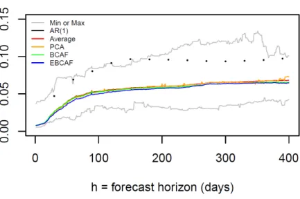
Next, we compare the out-of-sample MSE of each of the …ve forecast methods employed here: the AF, the PCA, the BCAF, the extended BCAF and the AR (1) model. Figure 4 plots the daily horizon results for these methods12_{, jointly with the minimum and} maxi-mum MSEs across all survey respondents. The …rst interesting feature is the comparison between the AR (1) model and the forecast-combination techniques discussed here – the AF, the PCA, the BCAF, and the extended BCAF. The AR (1) model is usually close to upper bound of the MSE for the forecasts in the data base, while the other four methods are all close to the lower bound in the very short horizons and are all below the mid-range in the medium/long horizons. This shows that forecast combination works in practice –in our case, the optimal combination of survey forecasts. These results mimic those obtained by Ang et al. (2007) and Faust and Wright (2013).

Figure 4 - Mean Squared Error (MSE)

Note: Max (Min) denotes the maximum (minimum) MSE, for each horizon, across all forecasters.

Next, Table 2 compares the MSE of the …ve methods discussed above for short horizons (30, 60 or 90 days). There is a pecking order : the extended BCAF is superior to the BCAF and the PCA, which in turn dominate the AF, which in turn dominates the AR (1) model.

For longer horizons (180 or 360 days), the extended BCAF is superior to the BCAF, which in turn dominates the AF, which in turn dominates the PCA, which in turn dominates the AR (1) model. This validates the view that the bias corrections performed either by the BCAF, or by the extended BCAF, are a useful device for forecasting using surveys.

As shown in Table 2 and Figure 5 (left panel), when we compare the extended BCAF with the BCAF, AF or the PCA, forecasting MSE reductions can reach up to 10% at the 30 days horizon and are signi…cant for the AF and the BCAF. MSE reductions vis-à-vis the AR (1) model can reach up to 49% for the extended BCAF.

Table 2 - Mean Squared Error (MSE) horizon h

(days) AR(1) PCA

Average Forecast BCAF Extended BCAF 30 0:0471 [0:0009] 0:0255[0:2794] 0:0264(0:0253) 0:0263(0:0080) 0:0239 60 0:0691 [0:0277] 0:0439[0:3255] 0:0446(0:1131) 0:0439(0:0805) 0:0409 90 0:0804 [0:0685] 0:0515[0:3667] 0:0525(0:1522) 0:0516(0:1198) 0:0491 180 0:0962 [0:0549] 0:0601[0:3312] 0:0594(0:1904) 0:0581(0:1902) 0:0564 360 0:0955 [0:1340] 0:0674[0:3876] 0:0672(0:2327) 0:0652(0:2234) 0:0645 Notes: The second and third columns show [in brackets] the p-values of the test of Diebold-Mariano (1995) which compares the Extended BCAF with the forecast in each column. The other columns show (in parenthesis) the p-values of the test of Clark and West (2007), which compares the Extended BCAF and the forecast in each column. In all cases, * indicates a rejection of the null at a 10% level. Bold …gures indicate the lowest MSE in each horizon.

We now test whether or not forecast errors di¤er in a statistical sense. Figure 5 (right panel) presents the equal-predictive-accuracy test of Clark and West (2007) for nested models at di¤erent horizons. Results suggest that, vis-à-vis the average forecast (and the BCAF), the extended BCAF can statistically reduce (at the 10% signi…cance level) out-of-sample MSE for horizons up to 30 days for the AF (and up to 60 days for the BCAF). Comparisons of the extended BCAF with the AR (1) model using a Diebold-Mariano (DM) test for equal variances shows that the former is statistically superior to the latter (at the 10% signi…cance level) at horizons up to 180 days. The DM test also indicates that the extended BCAF is not statistically di¤erent to the PCA-based forecast at all horizons; although the extended BCAF exhibits lower MSEs compared to the PCA-based forecasts for all horizons shown in Table 2.

Figure 5 - MSE comparison (left panel) and Clark and West (2007) test (p-values, right panel)

Note: On the right panel, the red line represents a p-value of 0.10. Ho: equal predictive accuracy.

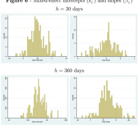
Next we use our consistent estimate of Et h(yt) to run a mixed-e¤ect model taking into account individual agent heterogeneity as in (24). Maximum likelihood estimates are presented in Table 3. First, note that the so-called both …xed-e¤ect parameters k0h and h0 are highly statistically signi…cant. Moreover, point estimates are very close to GMM estimates presented in Table 1. This is reassuring given the potential generated-regressor problem due to the use of a consistent estimate for Et h(yt) in its place.13 Regarding random-e¤ects estimates, the variance of _i is only statistically signi…cant at the shortest horizon (30 days), whereas that of i is signi…cant at all horizons except 180 days. Goodness-of-…t statistics reveal a high signal-to-noise ratio, since all the pseudo-R2 statistics are much closer to the unity than to the zero, suggesting that market professional forecasters attach more weight to common information (public and private) than to private idiosyncratic information. Indeed, for all horizons listed above, idiosyncratic information only accounts for about 20% to 30% of forecast variation. Therefore, common information accounts for 70% to 80%. Figure 6 plots the cross-sectional distribution of the estimates of kih and

h

i for selected horizons. It shows the importance of considering heterogeneity in estimating the a¢ ne-model parameters.

13_{Our estimate of E}

t h(yt) relies on asymptotic theory, but the sample size is relatively large, especially

in the time-series dimension. Perhaps that explains the small di¤erences between IV (GMM) estimates and the mixed-e¤ect estimates for all horizons.

Table 3 - Mixed-e¤ect model estimation fh i;t = khi + h iEt h(yt) + "hi;t kh i = k0h+ i; i N 0; 2 h i = h 0 + i; i N (0; 2) h (days) kh 0 h 0 2 2 Obs. Pseudo-R2 30 0:050 (0:005) 0:801(0:010) 1:2E(4:0E 04)03 6:1E 03 (1:6E 03) 9; 576 0:810 60 0:062 (0:004) 0:764 (0:009) 3:8E 05 (5:1E 05) 9:7E 04 (2:4E 04) 9; 413 0:762 90 0:068 (0:004) 0:758(0:009) 3:1E(3:9E 05)05 8:8E 04 (2:2E 04) 9; 330 0:752 180 0:062 (0:005) 0:757(0:011) 2:0E(3:8E 13)19 1:2E 03 (2:7E 03) 8; 610 0:709 360 0:048 (0:006) 0:770(0:012) 4:4E(8:8E 05)05 1:8E 03 (4:2E 04) 6; 655 0:689

Notes: Robust standard errors in parentheses. Pseudo-R2 is computed as 1-var(resid)/var(resid_null), where var(resid) denotes the residual variance of the model of interest and var(resid_null) represents

the residual variance of the null model (also referred to as the empty model or the intercept model).

Figure 6 - Mixed-e¤ect intercepts (kih) and slopes ( h i) h = 30 days 0 5 1 0 1 5 2 0 D e n s it y -.05 0 .05 .1 .15 blup intercept 0 5 1 0 1 5 D e n s it y .6 .7 .8 .9 1 blup slope h = 360days 0 1 0 0 2 0 0 3 0 0 4 0 0 D e n s it y .04 .045 .05 .055 blup intercept 0 5 1 0 1 5 2 0 D e n s it y .65 .7 .75 .8 .85 blup slope

Figure 7 - Actual (fh

i;t) and …tted ( cfi;th) individual forecasts for h = 30 days (left) and 360 days (right)

0 .5 1 1 .5 2 f_ it h (h = 3 0 d a y s ) 0 .5 1 1.5 2 f_ith_hat (h = 30 days) 45 degrees line 0 .5 1 f_ it h (h = 3 6 0 d a y s ) 0 .5 1 f_ith_hat (h = 360 days) 45 degrees line

Figure 7 presents a graphical comparison between the actual (fi;th) and …tted ( cfi;th) individual survey forecasts –the best linear unbiased predictors (BLUPs). Perfect forecasts would lie on the red 45-degree line. Figure 7 shows a good balance for the two horizons listed (30 and 360 days ahead).

Finally, using (27) we can measure the importance of the public (common) and the private (idiosyncratic) component of individual expectations using:

1 = VAR [Et h(yt)] VAR [Ei;t h(yt)] +VAR E ytj F P I i;t h VAR [Ei;t h(yt)] .

Table 4 below presents the results of this decomposition. Using Morris and Shin’s (2002) de…nition of public and private information, the public (common) component ac-counts for approximately 70 80% of total variance of individual expectations, whereas the importance of the private (idiosyncratic) term is relatively small, reaching at most 29% at the longest horizon. We can safely say that the importance of private (idiosyncratic) information is relatively small in forecasting Brazilian in‡ation. Figure 8 presents a picture of forecast components – common (public) versus idiosyncratic (private) – using Morris and Shin’s de…nition, for selected horizons. It con…rms the high relatively importance of public (common) information in forecasting in‡ation in Brazil.

Finally, using a dynamic panel-data model, estimated using the Arellano-Bond tech-nique, we test if the private (idiosyncratic) component of individual expectation, E ytj Fi;t hP I , does not Granger cause relevant Brazilian aggregate series. At the 5% signi…cance level, the monthly growth of the Brazilian target interest rate (SELIC), the stock market in-dex (IBOVESPA) and the country risk-premium (EMBI+BR) are not Granger-caused by E ytj Fi;t hP I . While we should expect individual idiosyncratic expectation components to be important for some agents and/or for some time periods, its average importance should be reduced across the market and time periods.

Table 4 - Variance decomposition of individual expectations h (days) _{VAR [E}i;t h(yt)] VAR [Et h(yt)] VAR E ytj Fi;t hP I

30 0:0722 (100%) 0:0581 (80%) 0:0141 (20%) 60 0:0512 (100%) 0:0400 (78%) 0:0111 (22%) 90 0:0460 (100%) 0:0352(77%) 0:0108(23%) 180 0:0382 (100%) 0:0278(73%) 0:0104(27%) 360 0:0356 (100%) 0:0251(71%) 0:0104(29%) Note: Figures in parentheses denote the relative importance of the variance terms.

Figure 8 - In‡ation and forecast components Common (public) versus idiosyncratic (private)

For h = 30 days (left) and 360 days (right)

-. 5 0 .5 1 1 .5 60 70 80 90 100 110 120 130 140 150 Months (Dec2010:May2018)

IPCA inflation EBCAF h=30days cross-section mean of E(yt;PI)

-. 5 0 .5 1 1 .5 60 70 80 90 100 110 120 130 140 150 Months (Dec2010:May2018)

IPCA inflation EBCAF h=360days cross-section mean of E(yt;PI)

Note: E ytj Fi;t hP I in red, IPCA in‡ation in black and Et h(yt) in blue.

4

Conclusion

This paper proposes a …nancial approach to economic forecasting which can be applied to data bases of surveys of forecasts. From a forecasting perspective, the focus on surveys is important, since Faust and Wright (2013) have shown forcefully that subjective forecasts of in‡ation seem to outperform model-based forecasts. We model the forecasting decision of an individual from …rst principles (i.e., microfounded ) and show that surveys of fore-casts obey an a¢ ne factor structure with a single factor which is the common component of the conditional expectation of the target variable. This holds in a context where indi-viduals only have access to public and private information with common and idiosyncratic components.

Our approach involves two layers of decision making. In the …rst, individuals choose the best forecast to be posted in the database containing surveys of forecasts. In the second, an econometrician uses the survey to forecast the target variable optimally. From the point of view of the econometrician, it is important to estimate the common factor

of the survey, which is the optimal forecast under an MSE risk function in a variety of contexts. We show how this can be performed using GMM-based estimates: the optimal forecast is a function of the consensus forecast of the survey (a cross-sectional average of forecasts) after appropriately …ltering out two bias terms. This links the …nancial approach of economic forecasting to the forecast-combination literature, where idiosyncratic risk of individual forecasts can be diversi…ed out.

Our results are applicable to two types of surveys with a large enough number of time-series observations (T ! 1): one of current surveys of forecasts, which possess a limited number of respondents (N < 1), and one that we have labelled as the Surveys of the Future, where the number of respondents is also large (N ! 1). The latter connects this paper with the literature on big data. In standard GMM moment estimation, we circumvent the curse of dimensionality that arises from the factor structure (large N ) by employing cross-sectional averages. In a big-data context, this allows the use of all the information contained in the survey, while estimating a parsimonious factor model, with only two bias terms –an intercept and a slope bias.

We apply the techniques advanced in this paper to forecast Brazilian in‡ation using the Focus Survey, organized by the Central Bank of Brazil. It is a unique panel database, which collects daily information from 298 registered professional institutions, which are followed throughout time with a reasonable turnover. There is a smaller active group of about 100 institutions that frequently update their forecasts. Forecasts are supplied at the daily frequency for a large array of macroeconomic time-series at di¤erent forecast horizons. Our sample covers forecasts for in‡ation rates from December 2005 to May 2018 (t = 1; :::; T = 150 months), and the forecast horizons range from h = 1; :::; H = 400 days. The …nal data base used in this paper contains 3; 594; 951 observations, forming a three-dimensional panel of agents.

We compare the truly out-of-sample mean-squared error (MSE) of …ve di¤erent forecast methods – four of them widely used in the forecasting literature: the method proposed here –the extended bias-corrected average forecast (extended BCAF), the average forecast (AF, the cross sectional average of forecasts), the principal-component analysis (PCA), the bias-corrected average forecast (BCAF), and the forecast of the AR (1) model for in‡ation, which is the best ARMA model in sample using the Schwarz Criterion. For short horizons (up to 90 days), there is a pecking order : the extended BCAF is superior to the BCAF and the PCA, which in turn dominate the AF, which in turn dominates the AR (1) model. For longer horizons, the extended BCAF is also superior to the other models in terms of MSE. When we compare the extended BCAF with the AF, MSE reductions can reach up to 10% at short horizons. Reductions vis-à-vis the MSE associated with forecasts of the AR (1) model can reach up to 49%.

References

[1] Ang, A., Bekaert, G., Wei, M., 2007. Do Macro Variables, Asset Markets or Surveys Forecast In‡ation Better? Journal of Monetary Economics 54, 1163-1212.

[2] Atak, A., Linton, O., Xiao, Z., 2011. A semiparametric panel model for unbalanced data with application to climate change in the United Kingdom. Journal of Econo-metrics 164 (1), 92-115.

[3] Athanasopoulos, G., Guillén, O.T.C., Issler, J.V., Vahid, F., 2011. Model Selection, Estimation and Forecasting in VAR Models with Short-run and Long-run Restrictions. Journal of Econometrics 164 (1), 116-129.

[4] Bai, J., 2009. Panel Data Models with Interactive Fixed E¤ects. Econometrica 77 (4), 1229-1279.

[5] Bakhshi, H., Kapetanios, G., Yates, T., 2005. Rational expectations and …xed-event forecasts: An application to UK in‡ation. Empirical Economics 30, 539-553.

[6] Ba´nbura, M., Giannone, D., Reichlin, L., 2011. Nowcasting, Chapter 7 in The Oxford Handbook of Economic Forecasting, Edited by Michael P. Clements and David F. Hendry, pp. 193-224.

[7] Bates, J.M., Granger, C.W.J., 1969. The Combination of Forecasts. Operations Re-search Quarterly 20, 309-325.

[8] Cameron, A.C., Trivedi, P.K., 2009, Microeconometrics: Methods and Applications, 8th Edition. Cambridge: Cambridge University Press.

[9] Capistrán, C., Timmermann, A., 2009. Forecast Combination with Entry and Exit of Experts. Journal of Business and Economic Statistics 27, 428-440.

[10] Clark, T.E., West, K.D., 2007. Approximately Normal Tests for Equal Predictive Accuracy in Nested Models. Journal of Econometrics 138, 291-311.

[11] Davies, A., 2006. A Framework for Decomposing Shocks and Measuring Volatilities Derived from Multi-Dimensional Panel Data of Survey Forecasts. International Jour-nal of Forecasting 22 (2), 373-393.

[12] Davies, A., Lahiri, K., 1995. A new framework for analyzing survey forecasts using three-dimensional panel data. Journal of Econometrics 68, 205-227.

[13] Diebold, F.X., 2012. A Personal Perspective on the Origin(s)

and Development of ‘Big Data’: The Phenomenon, the Term,

and the Discipline. Manuscript, University of Pennsylvania,

http://www.ssc.upenn.edu/~fdiebold/papers/paper112/Diebold_Big_Data.pdf [14] Diebold, F.X., Mariano, R.S., 1995. Comparing Predictive Accuracy. Journal of

Busi-ness and Economic Statistics 13, 253-263.

[15] Einav, L., Levin, J.D., 2014. The Data Revolution and Economic Analysis, in, Inno-vation Policy and the Economy, Josh Lerner and Scott Stern, editors. NBER Book: University of Chicago Press.

[16] Elliott, G., Komunjer, I., Timmermann, A., 2008. Biases in Macroeconomic Forecasts: Irrationality or Asymmetric Loss? Journal of the European Economic Association 6 (1), 122-157.

[17] Elliott, G., Timmermann, A., 2004. Optimal forecast combinations under general loss functions and forecast error distributions. Journal of Econometrics 122, 47-79. [18] Elliott, G., Timmermann, A., 2005. Optimal forecast combination weights under

regime switching. International Economic Review 46 (4), 1081-1102.

[19] Engle, R.F., Issler, J.V., 1995. Estimating common sectoral cycles. Journal of Mone-tary Economics 35 (1), 83-113.

[20] Engle, R.F., Kozicki, S., 1993. Testing for Common Features (with comments), Jour-nal of Business and Economic Statistics 11, 369-395.

[21] Faust, J., Wright, J.H., 2013. Forecasting In‡ation. Handbook of Economic Forecast-ing, Volume 2A, Chapter 1, p.3-56. Ed. Elsevier B.V.

[22] Forni, M., Hallim, M., Lippi, M., Reichlin, L., 2000. The generalized dynamic factor model: Identi…cation and estimation. Review of Economics and Statistics 82, 540 554. [23] Forni, M., Hallim, M., Lippi, M., Reichlin, L., 2005. The generalized dynamic factor model: One-sided estimation and forecasting. Journal of the American Statistical Association 100, 830-840.

[24] Gaglianone, W.P., Issler, J.V., Matos, S.M., 2017. Applying a microfounded-forecasting approach to predict Brazilian in‡ation. Empirical Economics 53 (1), 137-163.

[25] Gaglianone, W.P., Lima, L.R., 2012. Constructing Density Forecasts from Quantile Regressions. Journal of Money, Credit and Banking 44 (8), 1589-1607.

[26] Gaglianone, W.P., Lima, L.R., 2014. Constructing Optimal Density Forecasts From Point Forecast Combinations. Journal of Applied Econometrics 29 (5), 736-757. [27] Gaglianone, W.P., Lima, L.R., Linton, O., Smith, D.R., 2011. Evaluating

Value-at-Risk Models via Quantile Regression. Journal of Business and Economic Statistics 29 (1), 150-160.

[28] Geweke, J. (1977), “The dynamic factor analysis of economic time series”, in: D.J. Aigner and A.S. Goldberger, eds., Latent Variables in Socio-Economic Models. North-Holland, Amsterdam.

[29] Granger, C.W.J., 1969. Prediction with a generalized cost of error function. Opera-tional Research Quarterly 20 (2), 199-207.

[30] Granger, C.W.J., Newbold, P., 1986. Forecasting time series, 2nd Edition. Academic Press.

[31] Granger, C.W.J., Ramanathan, R., 1984. Improved methods of combining forecasting. Journal of Forecasting 3, 197–204.

[32] Hansen, L.P., 1982. Large Sample Properties of Generalized Method of Moments Estimators. Econometrica 50, 1029-1054.