Microfounded forecasting

Ensaios Econômicos

Escola de

Pós-Graduação

em Economia

da Fundação

Getulio Vargas

N◦ 766 ISSN 0104-8910

Microfounded Forecasting

Wagner Piazza Gaglianone, João Victor Issler

Os artigos publicados são de inteira responsabilidade de seus autores. As

opiniões neles emitidas não exprimem, necessariamente, o ponto de vista da

Fundação Getulio Vargas.

ESCOLA DE PÓS-GRADUAÇÃO EM ECONOMIA Diretor Geral: Rubens Penha Cysne

Vice-Diretor: Aloisio Araujo

Diretor de Ensino: Carlos Eugênio da Costa Diretor de Pesquisa: Humberto Moreira

Vice-Diretores de Graduação: André Arruda Villela & Luis Henrique Bertolino Braido

Piazza Gaglianone, Wagner

Microfounded Forecasting/ Wagner Piazza Gaglianone, João Victor Issler – Rio de Janeiro : FGV,EPGE, 2015

45p. - (Ensaios Econômicos; 766)

Inclui bibliografia.

Microfounded Forecasting

Wagner Piazza Gaglianone

João Victor Issler

Abstract

Our focus is on information in expectation surveys that can now be built

on thousands (or millions) of respondents on an almost continuous-time basis

(big data) and in continuous macroeconomic surveys with a limited number

of respondents. We show that, under standard microeconomic and

econo-metric techniques, survey forecasts are an a¢ne function of the conditional

expectation of the target variable. This is true whether or not the survey

respondent knows the data-generating process (DGP) of the target variable

or the econometrician knows the respondent’s individual loss function. If the

econometrician has a mean-squared-error risk function, we show that

asymp-totically e¢cient forecasts of the target variable can be built using Hansen’s

(Econometrica, 1982) generalized method of moments in a panel-data context,

when N and T diverge or when T diverges with N …xed. Sequential

asymp-totic results are obtained using Phillips and Moon’s (Econometrica, 1999)

framework. Possible extensions are also discussed.

Keywords: Forecast Combination, Big Data, Common Features, Panel

Data.

The views expressed in the paper are those of the authors and do not necessarily re‡ect those of the Banco Central do Brasil or of FGV. Also, all data manipulations were executed by employees of the Banco Central do Brasil. We are especially grateful for the comments and suggestions given by Scott Atkinson, Robert Engle, Antonio Galvão, Ra¤aella Giacomini, Alain Hecq, Bo Honoré, Fabian Krüger, Marcelo Moreira, Rafael Santos, Mark Watson, and Whitney Newey. We also bene…ted from comments given by the seminar participants of the International Symposium on Forecasting (Seoul); International Panel Data Conference (London); Latin American Workshop in Econometrics (São Paulo); XVI Annual In‡ation Targeting Seminar of the Banco Central do Brasil (Rio de Janeiro); and The Conference of the International Association for Applied Econometrics (London). Any remaining errors are ours. Both Gaglianone and Issler gratefully acknowledge the support from CNPq, FAPERJ, INCT and FGV on di¤erent grants.

y_{Research Department, Banco Central do Brasil. Email: [email protected]}

z_{Corresponding Author. Graduate School of Economics, Getulio Vargas Foundation, Praia de}

JEL Classi…cation: C14, C33, E37.

1

Introduction

Ang et al. (2007) argue that economists use four main methods to forecast in‡ation: time-series models of the ARIMA variety; structural models built upon the Phillips

Curve; methods using information embedded in asset prices – in particular, the term-structure of interest rates; and methods that employ survey-based measures provided by economic agents (consumers and/or professional forecasters). They …nd that

true out-of-sample survey forecasts (e.g. Michigan; Livingston) outperform a large number of out-of-sample single-equation and multivariate time-series competitors. Along the same lines, Faust and Wright (2013) argue that subjective forecasts of

in‡ation seem to outperform model-based forecasts in certain dimensions, often by a wide margin. They discuss some reasons why this is the case, which points out to the choice of boundary values and the fact that professional forecasters quite often

have access to econometric models and add expert judgment to these models. In a world where there is an increasing availability of reliable data provided electronically, it is interesting to examine how one could e¢ciently use this wealth of

information. Of course, there is already a large literature onbig data in statistics. It is certainly true that econometrics is currently bene…ting from it. However, what we see as lacking is interpretation – economic interpretation. One step in that direction

is to employ the tools of economics to be able to extend our current knowledge in an emerging …eld. This is one of the objectives of this paper.

In order to accomplish that, our focus is on the abundant information

con-tained in expectation surveys that can now be built on thousands (or millions) of respondents on an almost continuous-time basis. Using standard microeconomic and econometric techniques, we …rst ask what is the optimal survey response from the

point-of-view of a given respondent. As users of that information, it is important to us to consider an environment with three di¤erent setups: (i) when the survey respondent knows the data-generating process (DGP) of the response random

and users know what is the loss function being used; and (iii) when the respondent does not know the parameters of the DGP, the latter being approximated using a

location-scale model and quantile regression techniques, and the loss function being used by respondent is unknown to the users. Under these conditions, we show that the optimal forecast of a given survey respondent is an a¢ne function of the

condi-tional expectation of the target variable of the survey. Once we characterize this …rst layer of decision making, we can then ask how to use e¢ciently the informational content present in expectation surveys. Our answer uses structural microfounded

models, whereas the previous literature had focused on a reduced-form approach. If the …nal user of that information (the second layer of decision making) em-ploys a mean-squared-error (MSE) risk function, which is typically the case for the government, a central bank, a large risk-neutral …rm, etc., then, it is natural to extract from the survey the conditional expectation of the target variable1 _{– the}

optimal forecast from the point-of-view of the …nal user, e.g., an econometrician.

Because we had an a¢ne model for the optimal respondent’s decision, the second-layer problem reduces to a signal-extraction problem, where potentially the number of respondents and of time-series observations is large, i.e., N and T grow without

bound. In this context, we show how to solve this problem using Hansen’s (1982) generalized method of moments (GMM) in the sequential asymptotic framework of Phillips and Moon (1999), i.e., our method identi…es and proposes consistent and

e¢cient estimates of the optimal forecast of the target variable under the MSE risk function. Moreover, we also propose a solution for the case in which T diverges but N is …xed, which applies to some long standing surveys with a …xed number of

respondents throughout time.2

Although the a¢ne model of the …rst-layer decision making is a function of a latent variable (the conditional expectation), we are able to substitute it for the

target variable itself minus a martingale-di¤erence sequence (MDS) error term, thus expressing the cross-sectional moment condition in terms of this MDS, where its unforecastable properties can then be exploited using GMM. So, the moment

con-dition can ultimately be cast only in terms of observables and parameters. In this

1_{Of course, di¤erent risk functions in the second layer would imply extracting a di¤erent target.}

This is not a problem here, given that we have properly characterized the …rst-layer decisions.

2_{For example, theLivingston Survey of the Philadelphia FED, theWall Street Journal Survey}

setting, we confront forecasts with realizations to be able to identify and estimate consistently functions of the parameters of the a¢ne model when the number of

time-series observations gets large – large T. Our results hold in two di¤erent con-texts regarding the number of survey responses: when they are large(N ! 1)and when N is …xed.

Obviously, our primary focus is on forecasting. As Einav and Levin (2013) put it, “The most common uses of “big data” by companies are for tracking business processes and outcomes, and for building a wide array of predictive models. While

business analytics is a big deal and surely has improved the e¢ciency of many organizations, predictive modeling lies behind many striking information products and services introduced in recent years.” However, since our techniques allow the

identi…cation and estimation of the conditional expectation of the target variable, it immediately allows for the identi…cation of economic shocks to these target variables, which are key variables especially in macroeconomics and …nance; see the discussion

in Diebold (2012).

We should stress that we avoid dealing with sparse-data issues in big data, e.g., Belloni and Chernozhukov (2011, 2013) and Belloni, Chernozhukov, and Wang

(2011), because our focus narrows down to the relationship between optimal fore-casts and the conditional expectation of the target variable in the survey. Implicitly, each survey respondent could use several di¤erent covariates to compute their

opti-mal forecast. Indeed, all of these may be unknown to the user in the second layer of decision making (the econometrician). Because the number of respondents diverge, our techniques bene…ts from the information implicit in all of these forecasts, and

could ultimately be interpreted as an optimal forecast-combination method. Thus, our approach to big data is not related to data reduction techniques – where the key issue is the availability of too many regressors (Varian, 2014) – but on how to

optimally combine information.

The ideas in this paper are related to research done in three di¤erent …elds. From econometrics, it is related to the common-features literature after Engle and

Kozicki (1993). Indeed, we attempt to bridge the gap between a large literature on common features applied to macroeconomics, e.g., Vahid and Engle (1993, 1997), Issler and Vahid (2001, 2006) and Vahid and Issler (2002), Athanasopoulos et al.

fac-tors or to forecast combination, perhaps best represented by the work of Bates and Granger (1969), Granger and Ramanathan (1984), Palm and Zellner (1992), Davies

and Lahiri (1995), Forni et al. (2000, 2005), Stock and Watson (2002a,b, 2006), Elliott and Timmermann (2004, 2005), Timmermann (2006), Patton and Timmer-mann (2007), Issler and Lima (2009), Gaglianone et al. (2011), Gaglianone and Lima

(2012, 2014), and Lahiri, Peng, and Sheng (2013). From the theoretical literature on the incentives leading to optimal forecasts, our paper is related to the work of Laster et al. (1999), Ottaviani and Sorensen (2006), and Batchelor (2007). In this

context, it is also related to the literature on the role of loss functions, e.g., Elliott et al. (2008) and Capistrán and Timmermann (2009), and to the novel literature on informational rigidities, e.g., Mankiw and Reis (2010), Coibion and Gorodnichenko

(2012), and Andrade and Le Bihan (2013). Frombig data econometrics it is related to the work of Diebold (2012), Einav and Levin (2013), Varian (2014), Warin and Sanger (2014), and Joseph et al. (2014), although we could not …nd papers dealing

directly on how to optimally combine forecasts in the context of big data. Indeed, most of this literature is interested in dimension-reduction techniques for poten-tial regressors, such as classi…cation and regression trees (CART), random forests,

penalized-regression techniques such as the least absolute shrinkage and selection operator (LASSO) and least-angle regression (LARS), and elastic nets.

The rest of the paper is divided as follows. Section 2 introduces a

microfounded-based framework to study the forecast error under risk functions more general than the usual MSE. Section 3 presents a real-time forecasting exercise with data from a survey of Brazilian in‡ation expectations using the methods proposed here,

compar-ing the out-of-sample performance of di¤erent bias-correction approaches. Section 4 concludes.

2

Econometric Setup

2.1

Microfounded forecasting under a general risk function

The techniques discussed in this section are appropriate for forecasting a weakly

stationary and ergodic univariate process fytg using a large number of forecasts.

are generated using econometric models, but then the econometrician that observes these forecasts has no knowledge of them.

We label individual forecasts of yt, computed using information sets lagged h

periods, by fh

i;t, i= 1;2; : : : ; N, and t= 1;2; : : : ; T. Therefore, fi;th areh-step-ahead

forecasts of yt, formed at period t h; and N is the number of respondents of this

opinion poll regarding yt. In this section, we show that, in a variety of interesting

cases, optimal forecasts are related to Et h(yt) – the conditional expectation of yt,

computed using information lagged h periods – by an a¢ne function of the form3_:

f_i;th = h_iEt h(yt) +khi +"hi;t: (1)

As is well known, Granger (1969) was a pioneer in this literature. He considered that forecasters minimize a cost function, and that “cost functions that arise in

practice in economics and management situations are not likely to be quadratic in form, and frequently will be non-symmetric.” If the cost function is symmetric, and

additional regularity conditions hold for the density of yt, thenEt h(yt) is obtained

as the optimal forecast. In some special cases, optimal forecasts require a bias-correction term as in Et h(yt) +kih.

The subsequent literature on forecast optimization, e.g., Christo¤ersen and Diebold (1997), Elliott and Timmermann (2004), Patton and Timmermann (2007), and El-liott, Komunjer, and Timmermann (2008), have shown the inappropriateness of

using the conditional mean under a more general setup, which includes the use of an asymmetric loss function and even an unknown loss function.

In what follows, we consider a setup which has two layers of decisions to be

made. In the …rst layer, individuals (survey respondents) form their optimal point forecasts of a random variable yt by using a speci…c loss function under di¤erent

assumptions about knowledge of the DGP of yt. These optimal forecasts fi;th will

be available as survey results, where the number of respondents is potentially large, i.e., N ! 1, and these surveys can be periodically taken on a large number of di¤erent occasions, i.e., T ! 1. This setup describes reasonably well the current

abundance of knowledge in the big data literature. In the second layer of decisions, an econometrician will be the …nal user of this large number of forecasts. We

as-3_{Indeed, (1) is an encompassing model. Some results we derive below represent restrictions on}

sume that she/he operates under an MSErisk function, but this assumption can be modi…ed if need be. However, we believe it covers reasonably well some interesting

cases, which are of practical importance, e.g., the government, a central bank, a large risk-neutral …rm, etc. Hence, her/his optimal forecast in this second layer of decision making is Et h(yt).

The challenge here is to uncover Et h(yt) – the optimal forecast of the second

layer of decision making – from a potentially large set of survey responses, where cases of potential asymmetries or unknown loss functions previously studied are

taken into account. We investigate the relationship between the optimal forecast and the conditional expectation, based on the following cases: (1) Loss function known to the econometrician and DGP known by individual i, where the DGP may

take an analytic parametric form; (2) Loss function known to the econometrician and DGP known by individual i, where the DGP is approximated by a location-scale model with known parameters; (3) Loss unknown to the econometrician and

parameters of DGP unknown by individual i, the latter being estimated by the individual using standard quantile-regression techniques and a location-scale model.

Loss and DGP known – (Cases (1) and (2))

Assume that there is an amount of individuals forecasting yt conditional on Ft h,

where Ft h is the sigma algebra of all the variables contained in the conditioning

set used by all the agents. Each individual chooses an optimal forecast feh i;t by

minimizing their respective expected loss function Li_{, e.g., Granger and Newbold}

(1986). In this section, we assume that the agent in the second layer of decision making – the econometrician – has full knowledge of the Loss function used by individual agents. So, there is full disclosure not only of survey-forecast results but

also of the Loss function from the part of survey respondents. This last assumption will be relaxed in the next section.

Assumption A1 (Loss function) Li _{depends solely}4 _{on the forecast error e}i t;t h

yt fei;th, that is,Li = L(eit;t h).

4_{This is the same Assumption L1 of Patton and Timmermann (2007). According to them,}

Therefore, the optimal (point) individual forecasts ofyt are obtained as follows:

e

f_i;th arg min

f E

Li(yt;f)j Ft h (2)

where f 2 R are all possible choices of the i-th forecaster and E(: j Ft h) denotes

the conditional expectation given Ft h.

An important issue regarding the information set used by each agent is that all use the same information, which should be regarded as public information. Hence, there is no private information in our context, and di¤erent forecasts arise because agents use a di¤erent Loss function. Also, we treat public information as free, since the minimization problem in (2) has no constraints regarding its cost. These

features will have bearing when we discuss our theoretical results vis-à-vis those of the macroeconomics literature on forecasting.

A natural assumption about the shape of the agent’s loss function is that if one

forecasts without error, then no forecast loss arises, but, if there is an error, the larger it is, the greater will be the loss:

Assumption A2 (Shape of the Loss function) The loss function exhibits the fol-lowing properties: (i) Li_{(0) = 0; (ii) L}i_(e

i) is continuous, homogeneous and

non-negative 8ei 2R; and (iii) Li(ei) is monotonic non-decreasing (forei >0

or ei <0), and di¤erentiable at least twice almost everywhere.

In practical terms, the symmetry of the loss function might be a restrictive hypothesis to be considered by an econometrician. Granger and Newbold (1986, p.125) provide two examples of situations where nonsymmetrical cost functions arise.

In these cases, it would be interesting to check if the agent forecast is optimal under a broader class of loss functions. A simple way to consider an asymmetric function, and account for some "degree of asymmetry", is given by the following assumption:

Assumption A3 (Asymmetry of the Loss function) The loss function Li_(e i) can

be decomposed as Li_(e

i) = gi(ei)hi(ei), where gi(ei) is a non-negative and

symmetric function about ei = 0; gi0(ei) and gi00(ei) exist almost everywhere;

hi_(e i) =

8 < :

i

1 ; ei <0 i

2 ; ei >0

Assumption A4 (DGP - stationarity and regularity of the CDF) The univariate time series yt is a weakly stationary and ergodic process and the conditional

cumulative distribution function (CDF) of yt, givenFt h (denoted byFt;t h( )

or Ft( j Ft h)), is absolutely continuous, with continuous densities ft;t h

uni-formly bounded away from0and 1at the pointsF_{t;t h}1 ( );8 2(0; 1), where

denotes the quantile level with respect to the (conditional) CDF ofyt.

Assumptions A2 and A3 are standard in the literature (e.g. Granger and

New-bold, 1986; Patton and Timmermann, 2007). Note that A3 includes the symmetric case when ₁ = ₂. It is quite general, covering a great deal of loss functions commonly mentioned in the literature, such as: mean squared error (MSE), mean

absolute error (MAE), asymmetric linear (Lin-Lin), asymmetric quadratic, among many others. A4 is just a technical assumption on the DGP of yt.

Based on assumptions A1-A4, we next present Proposition 1, which generalizes

the results in Granger (1969) and states two important results: (i) asymmetric loss functions generate departures of the optimal forecast from the central tendency (e.g. median) of the conditional distribution of yt; and (ii) for the same DGP, the higher

the degree of asymmetry in the loss function the greater will be the distance between the optimal forecast and the conditional median.

Proposition 1 (Asymmetric Loss) Denote by M edt h(yt) the conditional median

of yt. If A1-A4 hold, then: (i) If 1 6= 2 then Ft;t h(fei;th)6= 0:5, where Ft;t h is the

conditional CDF of yt; (ii) If 1 > 2 then fei;th < M edt h(yt); (iii) If 1 < 2 then

e

fh

i;t > M edt h(yt); and (iv) for two forecasters iandj such that i1= i2 <

j

1=

j

2 <1, then, feh

i;t >fej;th > M edt h(yt):

Corollary 2 (Symmetric Loss) If A1-A4 hold, and ₁ = ₂, thenfeh

i;t =M edt h(yt).

Hence, without asymmetry, i.e., if 1 = 2, then, the optimal forecast is the

conditional median of yt. By considering additional assumptions on the DGP of yt,

we obtain the well-known optimality result of the conditional mean, due to Granger

(1969, Theorem 2).

symmetric function about its conditional mean Et h(yt) = 1

R

1

ytft;t h(y)dy, and if

1 = 2 then fei;th =Et h(yt).

It is interesting to note that an optimal forecast obtained from a symmetric loss function such as MSE implies that feh

i;t = Et h(yt). Moreover, the classical result

of Granger (1969), in which the optimal forecast equals the conditional mean of yt

under a MSE loss function, can be viewed as a special case of Proposition 1.

The exact relationship between the optimal forecast’s quantile level i, with

respect to the CDF of yt, and the parametersf 1; 2g can be obtained if one

con-siders a more restrictive assumption on the class of loss functions. The next corollary presents an example.

Corollary 4 (Granger and Newbold (1986): Linear loss function) If A1-A4 hold

and the loss function is a Lin-Lin function, i.e., if L(ei) =

8 > > < > > :

1ei ; ei <0

0 ; ei = 0

2ei ; ei >0

,

where ₁; ₂ >0, then, feh

i;t =Ft;t h1 ( i) in which i = 2=( 1+ 2).

Under a symmetric loss function such as the MSE, the only forecast that is

unbi-ased5_{is the optimal forecast given byf}eh

i;t =Et h(yt). However, under an asymmetric

loss function, we should expect that the optimal forecast will di¤er from the con-ditional mean. Intuitively, an asymmetric loss with, say, ₁ > ₂, indicates that

the negative forecast errors are relatively more costly to the forecaster. Thus, an individual forecaster will choose an optimal forecast that corresponds to some low quantile of yt (i.e., i < 0:5) and therefore it is natural to obtain a result where

positive errors are more likely to be observed with historical data – which explains the forecast bias.

Granger (1969) argues that symmetry of both the loss function and the

condi-tional density of yt is not a su¢cient condition for the optimum predictor to be

equal to the conditional mean. In fact, he provides a counter-example in which the conditional mean would be sub-optimal under symmetric functions (both loss

and the PDF). In order to better understand the relationship between the optimal forecast and the conditional mean, we next assume speci…c parametric versions for the DGP, as follows:

Proposition 5 (DGP - parametric PDFs) If A1-A4 hold and the conditional PDF of yt is: (i) Gaussian, Two-piece Normal, or Logistic, then, fei;th = khi +Et h(yt);

(ii) Log-normal or Weibull, then, feh i;t =

h

iEt h(yt); (iii) Beta(a = 1; b > 0), then,

e

fh

i;t =khi + hEt h(yt); (iv) Beta(a >0; b = 1), then, fei;th = hi'(Et h(yt); i), where

'(Et h(yt); i) = exp(_{Et h}ln(₍i_y)_t)) and i Ft;t h(fei;th).

With the exception of case (iv) above, it is instructive to note that Proposition 5 delivers an encompassing result that:

e

f_i;th = h_iEt h(yt) +kih; (3)

where di¤erent parametric CDFs deliver di¤erent restrictions on either intercepts

and/or slopes of the a¢ne function (3). Di¤erent intercepts and slopes are usually a result of the interaction between the DGP and the Loss function, in some cases being linked to asymmetry of the Loss function. If both are asymmetric, as in (iv)

above, we do not obtain an a¢ne function, but a nonlinear factor model onEt h(yt).

Knowledge of the Loss function (by the econometrician) and the DGP (by the agent) is too stringent an assumption, making it of little practical interest. Thus, we

now turn into a more realistic case where we assume a location-scale model for the DGP of yt. This broad class of DGPs was used by Patton and Timmermann (2007),

among others. Several parametric DGPs belong to it, such as the Normal

distrib-ution, Elliptical, Cauchy, Uniform, Logistic, Student’s t, and Generalized extreme value. The class also includes most common volatility processes, such as ARCH and stochastic volatility. It is not only broad but also very convenient, because it can

naturally be investigated through the lens of the quantile-regression framework with linear conditional quantiles.6

Assumption A5 (DGP - location-scale) The DGP of yt follows a location-scale

model, with conditional mean and variance dynamics de…ned asyt =Xt;t h0 +

X0

t;t h t, in which ( tjFt h) i:i:d: F ;h(0;1), where F ;h(0;1) is some

distribution with zero mean and unit variance, which depends on h but does not depend on Ft h; Xt;t h 2 Ft h is a m 1 vector of covariates (which

includes the intercept, and that can be predicted using information available

6_{The linear quantile regression setup could be further extended to consider models with}

at time t h) and = [ 0; 1;:::; m 1] and = [ 0; 1;:::; m 1] are m 1

vectors of parameters.7

Notice that no parametric structure is placed onF ;h( )and the covariates a¤ect

both the location and the scale of the conditional distribution of yt. Moreover, A5

implies that: (i) Q (yt j Ft h) = 0( ) + 1( )xt;t h for some 2 [0;1]; and (ii)

E(yt j Ft h) = Et h(yt) = 0 + 1xt;t h; where Q (:) is the conditional quantile

of yt, [ 0( ); 1( )] depends on ( ; ), Li and F ;h(0;1); and j

1

R

0

j( )d for

j = f0; 1g: The previous expressions for both the conditional quantiles and the conditional expectation of yt (under A5) will be exploited next to deliver a linear

connection between the optimal forecast and the conditional mean.

Proposition 6 (Location-scale model) If A1-A5 hold, then: (i) the optimal forecast is a linear function of the conditional mean of yt, so thatfei;th =khi + hiEt h(yt); (ii)

in the absence of scale e¤ects on the DGP ( ₁ = ₂ =:::= _{m 1} = 0)it follows that

h

i = 1, for all i, i.e., fei;th =khi +Et h(yt).

Here, scale e¤ects generate heterogeneity on the slopes of the a¢ne structure. On

the other hand, the intercept is a function of both scale and location parameters. We now turn into the case where the Loss function is unknown by the econometrician. Moreover, the DGP is also unknown by the agent and the econometrician. However,

it can be approximated using the location-scale model by the agent in forming her/his optimal forecast. In other words, the parameters and , associated with the location-scale model, can be consistently estimated as we shall see next.

Loss unknown and parameters of DGP unknown (Case (3))

So far, we have assumed that the Loss function is known by the econometrician and that the DGP of yt is known to the survey respondent who is forecasting yt. In

practice, only the survey respondent knows her/his own Loss function, but not the

econometrician. Moreover, it is not realistic to assume that either the respondent or the econometrician know the DGP. In this context, we consider the case where the econometrician only observes a survey of individual forecasts and the target variable

7_{For ease of notation, and without loss of generality, we assume that X}0

t;t h = (1; xt;t h)is a

2 1 vector, = ( 0; 1)0, and = ( 0; 1) 0

yt, but has no information at all about the individual loss functions previously used in

the …rst layer of decision making. Moreover, in the …rst layer, the survey respondent

does not know the DGP and has to estimate the parameters of the location-scale approximation.

Now, an optimal forecast of the form:

e

f_i;th =kh_i + _ihEt h(yt); (4)

obtained in the previous section, is not feasible. Despite that, because the class of location-scale models is relatively broad, we assume that the unknown DGP falls

within this class (A5) and that survey respondents employ the location-scale model to approximate the unknown DGP, which parameters must then be estimated.

A natural way for survey respondents to estimate (4) is by using

quantile-regression techniques, pioneered by Koenker and Bassett (1978), with further devel-opments discussed in Koenker (2005). Indeed, under standard assumptions about

the data, which are likely to hold in our context, it is possible for the survey re-spondent to estimate consistently kh

i, hi, andEt h(yt). If we denote bykbih, chi, and

b

Et h(yt) the respective estimators of kih, hi, and Et h(yt), the optimal (feasible)

survey responses are:

f_i;th =kbh

i +chiEbt h(yt); (5)

given the assumption that survey respondents use the location-scale model as an approximation.

Notice that we have made the distinction between the optimal forecast feh i;t and

its feasible counterpart fh

i;t which requires the estimation of khi, hi, and Et h(yt),

i.e., equation (4) versus (5). We now use a technical assumption that guarantees the existence of quantile-regression consistent estimates.

Assumption A6 De…ne[kbh

i;chi] = [b0( i) c_c0

1b1( i);

b1( i)

c1 ], where[b0( i);b1( i)]

are the resulting estimates (intercept and slope) of a standard linear quantile

regression of yt onto[1;xt;t h]at quantile level i. In addition, let the average

coe¢cients bj = PK_k=1bj( k) k, for j = f0; 1g, be computed as Riemann

sums over a grid ofK equidistant quantile levels k 2[ 1; 2; :::; K];such that

k = _Kk₊₁ and k = _K1₊₁ for k = [1; :::; K]. Also assume that regularity

continuous and Riemann-integrable on [0;1].

Proposition 7 If A1-A6 hold, then, the optimal (feasible) forecast ofyt conditioned

on Ft h is of the form: fi;th = khi + hiEt h(yt) +"hi;t, where "hi;t accounts for …nite

sample parameter uncertainty, and [kbh

i;chi] are consistent estimates of [kih; hi].

Notice that the case of unknown Loss function and DGP is similar to the two previous cases. Adding and subtracting kh

i + hiEt h(yt)to (5), leads to:

f_i;th =k_ih+ h_iEt h(yt) +"hi;t; (6)

where it becomes clear that "h i;t =

h b

kh i kih

i

+hch_iEbt h(yt) hiEt h(yt)

i

re‡ects

the small-sample error in approximating the unknown DGP8_{. Indeed, with one}

ex-ception, (6) encompasses all cases covered above, which are special cases re‡ecting speci…c parameter restrictions. Next, we will employ the encompassing model (6)

as a starting point to propose a way to identify and estimate consistently (and e¢ciently in a GMM context) the random variable Et h(yt).

As is clear from above, quantile-regression techniques allowed the estimation of

b

Et h(yt), kbih and c

h

i, but this is only available for the individual forecaster in the

…rst layer of decision making, since we assumed that only the survey respondent knows her/his own Loss function, but not the econometrician. The respondent will

deliver a bias and error ridden conditional expectation to the …nal user of the survey in the second layer – the econometrician, i.e., equation (6). So, from the point of view of the second layer, we are facing a typical signal-extraction problem, which

we solve exploiting the fact that forecasts are functions of Ft h, leading naturally to

errors that do not depend on Ft h. This can be the basis of a

generalized-method-of-moment estimate of _Et h(yt)as we discuss next.

Identi…cation and GMM estimation of Et h(yt)

Consider an econometrician who only observes a survey of individual forecasts fh i;t

(all optimal and feasible, in principle) and the target variable yt, but has no

in-formation at all about the DGP and the individual loss functions previously used

8_{As it is clear from the text, an optimal forecast "approximation error" "}h

i;t fi;th fei;th arises

in the …rst layer of decision making. Because the class of location-scale models is relatively broad, we assume that the econometrician will employ this class of models

to approximate the unknown DGP9_{. From our previous results, it is natural for the}

econometrician to use:

f_i;th =k_ih+ h_iEt h(yt) +"hi;t: (7)

As argued above, this encompasses the previous cases of Loss and DGP known,

and of Loss and DGP unknown10_{. Equation (7) is a three-dimensional panel, with}

t = 1; :::; T, i = 1; :::; N, and h = 1; :::; H. Although the horizon can in principle increase without bound, when forecasting one usually keeps H small. Recall that,

in a stationary-ergodic world, asH increases, conditional forecasts rapidly converge to their unconditional counterparts, making the case for large H unappealing. So, our framework entails two interesting cases. The …rst is T ! 1, N ! 1, and

small H, which applies to large surveys taken across time11_{. The second is T !} 1, with small N and H, which applies to some long standing surveys with an almost constant number of respondents throughout time, e.g., theLivingstonSurvey of the Philadelphia FED, available since 1959 on a biannual basis, the Survey of Professional Forecasters, available since 1968 on a quarterly basis, or theWall Street Journal Survey of Forecasters, available since 2003 on a monthly basis.

Even if H is small, the system of equations (7) has too many parameters when

N is large, which poses a problem for identi…cation ofEt h(yt). However, we do not

need the identi…cation of all kh

i and hi, i= 1; :::; N, to be able to identify Et h(yt).

Indeed, under suitable conditions, we only need to know their respective means.

Averaging (7) across i, assuming that _N1

N

X

i=1

"h i;t

p

!0, allows identifying Et h(yt) as

as function of three means alone:

Et h(yt) = plim

N!1

0 B B B B @

1

N N

X

i=1

fh i;t N1

N

X

i=1

kh i

1

N N

X

i=1

h i

1 C C C C

A; (8)

9_{The use of the location-scale class can be generalized, in principle, but we leave this for future}

research.

10_{There is one exception noted above.}

11_{Examples include large cross-sectional repeated surveys, where individuals are re-sampled with}

as long as all the terms in parenthesis in (8) converge in probability. The only

problem here is that kh ₌ 1

N N

X

i=1

kh

i and h = N1 N

X

i=1

h

i are not known. Next, we

discuss their estimation.

Our proposed approach to identify and estimate Et h(yt) is to employ the

gen-eralized method of moments (GMM), relying on T asymptotics. However, the fact

that Et h(yt) is a latent variable is a serious drawback, since the moments used in

GMM estimation must be a function of observables and parameters alone. Following Issler and Lima (2009), one can always decompose the series ytintoEt h(yt)and an

unforecastable martingale-di¤erence component h

t, such thatEt h( ht) = 0, so that:

yt=Et h(yt) ht: (9)

Thus, combining (7) and (9) leads to:

f_i;th = k_ih+ h_i(yt+ ht) +"hi;t (10)

= k_ih+ h_iyt+vhi;t; (11)

where vh

i;t hi ht +"hi;t is a composite error term. Notice that, by construction,

E ht j Ft h = 0, so, E vhi;t j Ft h = 0 if one assumes that E("hi;t j Ft h) = 0. In

the context where T; N ! 1, it is reasonable to expect that the approximation error "h

i;t vanishes.

Starting withE vh

i;t j Ft h = 0, using the law of iterated expectations and valid

observable instruments zt s, where zt s 2 Ft h, s h, we obtain:

E f_i;th k_ih h_iyt zt s = 0; (12)

which is valid for all i= 1; :::; N,t = 1; :::; T, andh= 1; :::; H. The system (12) has

2N H parameters and (at least)2N H moment conditions, provided thatdim(zt s)>

2, which is critical for identi…cation. Despite that, one problem remains: asN ! 1, the amount of parameters in (12) diverges, which goes against consistency. Notice, however, that T ! 1 poses no such problem.

time-series dependence. It relies on T-asymptotics and applies for the case where

N is …xed and the case where N ! 1. Notice that these are exactly the two

interesting cases alluded above. We …rst discuss T ! 1, N ! 1, with small

H. Driscoll and Kraay’s solution to the curse of dimensionality was to take cross-sectional averages of terms such as fh

i;t khi hiyt zt s. In their context, the

parameters to be estimated by GMM did not depend on i, although the data did. Here, both parameters and the data depend on i. Despite that, one can still use cross-sectional averages to reduce parameter dimensionality12_{, leading to:}

E

h

fh

;t kh hyt zt s

i

= 0; (13)

t = 1; :::; T, and h = 1; :::; H, where fh ;t = N1

N

X

i=1

fh

i;t, kh = N1 N

X

i=1

kh

i and h =

1 N N X i=1 h

i, represent cross-sectional averages for each h.

As argued above, since we need not know the individual coe¢cientskh

i and hi,

but only their means to be able to identify and estimate Et h(yt) from a survey of

forecasts, and since Et h(yt) does not vary acrossi, averaging across i as in (13) is

an interesting strategy to recoverEt h(yt). As long as these cross-sectional averages

converge, GMM using time-series restrictions delivers consistent estimates of the

respective parameter means. Once one deals successfully with consistency, one can start worrying about e¢ciency in a GMM context.

One way to exploit all possible moment conditions implicit in (13) is to stack all

the restrictions across h (…nite) as:

E 2 6 6 6 6 6 4 0 B B B B B @ f1

;t k1 1yt

f2

;t k2 2yt

.. .

fH

;t kH Hyt

1 C C C C C A

zt s

3 7 7 7 7 7 5

= 0; (14)

where our problem collapses to one where we haveH dim(zt s)restrictions and2H

parameters to estimate. As before, over-identi…cation requires that dim(zt s)> 2.

Given a choice ofH, GMM estimation of (14) is e¢cient. A less e¢cient alternative

12_{Provided thatz}

to estimate the whole stacked system (14) is to estimate separately (13) for every horizon h, which could also be attempted for computational reasons.

In the context of N; T ! 1, with H small, we now discuss the less stringent case where we …rst let N ! 1 and then let T ! 1, using the sequential as-ymptotic framework of Phillips and Moon (1999). Under suitable conditions, the

cross-sectional averages in (13) and (14) would converge in probability to a unique

limit as N ! 1, i.e., plim

N!1 1 N N X i=1 h

i = h, h 6= 0, h < 1, plim N!1 1 N N X i=1 kh

i = kh,

kh _{< 1, and plim} N!1 1 N N X i=1 fh

i;t = fh;t, fh;t < 1, for all t = 1;2; ; T. Then, a

key condition for T-consistent estimation is that (13) and (14), evaluated at these limits are a unique solution for each of them respectively. Take now moments (13),

considering that N ! 1:

E fh_;t kh hyt zt s = 0; or, (15)

E

"

h h

t +plim N!1 1 N N X i=1

"h_i;t

!

zt s

#

= 0: (16)

If, in addition, _N1

N X i=1 "h i;t p

!0, as N ! 1, (16) collapses to:

E h ht zt s = 0; (17)

t = 1; :::; T, and h = 1; :::; H, where (17) is attained by construction, since h t is a

martingale-di¤erence and must be orthogonal to all series dated t hor before. In this context, GMM provides a consistent estimate for parameter means as T ! 1. To prove it, …rst de…ne h = [kh_; h_{]0 and consider the following assumptions:}

Assumption A7 Let"h_t = "h_1;t; "h_2;t; ::: "h_N;t 0 be aN 1vector stacking the errors

"h

i;t associated with all possible forecasts. Assume that the vector process "h

t is covariance-stationary and ergodic for the …rst and second moments,

uniformly on N, and that E "h

i;t = 0 for all i and t, given h. Furthermore,

we assume that

lim N!1 1 N2 N X i=1 N X j=1

E "hi;t"hj;s = 0; (18)

Assumption A8 We assume that plim N_!1 1 N N X i=1 h

i = h 6= 0, h <1, plim N_!1 1 N N X i=1 kh i =

kh_{, k}h _{<1, and plim} N!1 1 N N X i=1 fh

i;t =fh;t, fh;t <1, for all t = 1;2; ; T.

Assumption A9 We assume that the identi…cation conditions for GMM estimation are met and that there is a unique set of values h₀ = [kh

0; h0]0,h= 1;2; ; H,

that solve either (14) or (13) for each h separately13_{. We further assume}

that the additional regularity conditions used by Hansen (1982) in proving

T-consistency of GMM estimates bh = [kbh_;ch_]0 _{are met as well.}

Assumption A7 guarantees that the errors "h

i;t can be diversi…ed away, and that

cross-sectional dependence is not a problem. It is required in a GMM context in

order to ensure that Et h plim N!1 1 N N X i=1 vh i;t !

= 0. This serves as a basis to obtain

either (13) or (14), when N ! 1. Notice that, although this is an assumption here,

it can be tested using standard over-identifying restrictions tests. Assumption A8 just requires …nite convergence of di¤erent cross-sectional averages, which bounds the degree of cross-sectional and time-series dependence due to spatial dependence.

They are expected to hold on a stationary-ergodic context. Assumption A9 deals with GMM identi…cation and is standard in the literature. We can now state an important result, which allows for consistent estimation of _Et h(yt).

Proposition 8 If A1-A9 hold, then, the feasible Extended BCAF (Bias Corrected Average Forecast) _N1

N

X

i=1

fh i;t kch

ch , based onT-consistent GMM estimates

bh

=hkbh_;chi0_;

obeys plim (N;T!1)seq

1 N N X i=1 fh i;t kch

ch

!

= Et h(yt), where (N; T ! 1)seq denotes the se-quential asymptotic approach proposed by Phillips and Moon (1999), when we let …rst N ! 1, and then let T ! 1.

We now turn into the more complicated case where in the sequential asymptotics we let …rst T ! 1, and then N ! 1, or, that we let T ! 1 with N …xed. The critical issue of letting T ! 1…rst is that, when we take cross-sectional averages as

in (13) or (14), but N is not large, we have to guarantee that all possible ensemble

13_{Since the restrictions are linear, the} h

averages are identi…ed. When we assume the opposite sequential order, we have only to worry about identi…cation of a single limit case.

An added complication is that _N1

N

X

i=1

"h

i;t does not vanish in probability. Despite

that, A7 imposes that E "h

i;t = 0 for all i and t, given h. This is not su¢cient to

guarantee that moments (13) and (14) can be cast in terms of h

t alone. However,

employing the more restrictive assumption that E("h

i;t j Ft h) = 0 is su¢cient to

validate (13) and (14). Thus, we employ the following assumptions outlined next:

Assumption A10 Let"h

t = "h1;t; "h2;t; ::: "hN;t 0

be aN 1vector stacking the errors

"h

i;t associated with all possible forecasts. Assume that the vector process "h_t is covariance-stationary and ergodic for the …rst and second moments,

uniformly on N, and that E("h

t j Ft h) = 0 for all t, givenh.

Assumption A11 De…ne _N1

N

X

i=1

h

i = h and N1 N

X

i=1

kh

i =kh. We assume that, for

allN, the identi…cation conditions for GMM estimation are met and that there

is a unique set of values h₀ = [kh

0;

h

0]0, h= 1;2; ; H, that solves either (14)

or (13) for eachhseparately. We further assume that the additional regularity conditions used by Hansen (1982) in proving consistency of GMM are met as

well.

We now turn to the analogous estimation result when we reverse the order of

sequential asymptotics: …rst T ! 1and thenN ! 1, or, that we letT ! 1with

N …xed.

Proposition 9 If A1-A6 and A10-A11 hold, then, the feasible Extended BCAF (Bias Corrected Average Forecast) 1

N N

X

i=1

fh i;t kch

ch , based on T-consistent GMM

esti-mates bh = kbh_;ch 0

, obeys plim

T!1 1 N N X i=1 fh i;t ckh

ch

!

=Et h(yt), where we let T ! 1,

with N …xed. The convergence to Et h(yt) also happens when we let …rst T !

1 and later let N ! 1, that is, plim (T;N!1)seq

1 N N X i=1 fh i;t kch

ch

!

= Et h(yt), where

Notice that assumptions A10 and A11 su¢ce to provide T-consistent GMM estimates for all bounded N. Indeed, …xed N is a special case of (T; N ! 1)seq,

where we do not let N diverge afterT ! 1, the context being identical otherwise. So far, under double asymptotics, we discussed the sequential convergence ap-proach, either (N; T ! 1)seq or(T; N ! 1)seq, for the Extended BCAF estimator.

Next, we ask under which conditions we can establish a link between sequential convergence and joint convergence. Following Phillips and Moon (1999), we state the formal conditions for the sequential convergence to imply joint convergence in

our setup.

Assumption A12 Let …rst holdN,T, andh…xed, and de…neY1 = _N1

N

X

i=1

fh i;t kch

ch

!

.

Letting now T ! 1, this de…nes plim

T!1

Y1 Y2 =

0 B B B @ 1 N N X i=1 fh i;t N1

N X i=1 kh i 1 N N X i=1 h i 1 C C C A. If

both N; T ! 1, this de…nes plim

N;T!1

Y1 Y3 = yt+ th = Et h(yt). We

as-sume that Y1, Y2, and Y3 are random variables on the same probability space ( ;F; P).

Assumption A13 lim sup

N;T

P fkY1 Y2k> "g= 0;8" >0;wherekAkis the

Euclid-ean norm (tr(A0_A))1=2

.

Proposition 10 If A1-A13 hold, then, both feasible extended BCAFs _N1

N

X

i=1

fh i;t ckh

ch

!

and _N1

N

X

i=1

fh i;t kch

ch

!

, based respectively onT-consistent GMM estimates bh = kbh_;ch 0

andbh =hkbh_;chi_{;obey plim}

(T;N!1) 1 N N X i=1 fh i;t ckh

ch

!

= plim (N;T!1)

1 N N X i=1 fh i;t kch

ch

!

=_Et h(yt),

regardless of the order in which N and T diverge.

Under di¤erent assumptions, our results above imply that we can estimate con-sistently Et h(yt), respectively, as follows:

b

Et h(yt) =

1 N N X i=1 fh i;t kbh

ch , or,

b

Et h(yt) =

1 N N X i=1 fh i;t kbh

ch

depending on whether we let …rst N ! 1, and then let T ! 1, or, we either let …rst T ! 1, and then letN ! 1, or holdN …xed afterT ! 1. In any case,

esti-mation of kh_; h

or ofhkh_; hi _{is performed by GMM underT-asymptotics. These}

estimates of Et h(yt) can be viewed as bias-corrected versions of survey forecasts.

If the mean kh _{or k}h _{is zero and the mean} h _or h _{is unity, these estimates}

converge to the same probability limit of the average (consensus) forecast _N1

N

X

i=1

fh i;t,

which has a long history in the forecasting literature.

2.2

Discussion

When considering a survey of forecasts where the number of respondents and of time observations is large – big data, and also the case where the number of time observations is large but the number of respondents is …xed – standard continuous macroeconomic surveys, we apply the tools of the literature on optimal forecasts in the time-series dimension and model the forecasting decision of an individual from

…rst principles. This constitutes the …rst layer of decision making. In our con-text, heterogeneity is a consequence of agents using di¤erent Loss functions, which generate cross-sectionally diverse optimal forecasts. Despite that, each forecast is

related to the conditional expectation of the target variable in the survey by an

a¢ne structure, where there is an intercept and slope bias due to the interaction between an asymmetric Loss and knowledge of the DGP. This a¢ne factor setup

can be exploited as a structural model for the conditional expectation.

Focusing on the conditional expectation de…nes the object of the second layer of decision making, when the user of the …nal information in the survey has an MSE

risk function, e.g., central banks, the government, large …rms, etc. The way we identify the conditional expectation can be viewed as a combination of cross-sectional averages with standard GMM moment conditions along the time dimension, where

the a¢ne structure o¤ers natural orthogonality restrictions allowing the estimation of bias-correction terms. We circumvent the curse of dimensionality that arises from the factor structure (large N) by employing these cross-sectional averages. In

a big-data context, this allows the use of all the information contained in the survey, while entailing the estimation of a parsimonious factor model.

For instance, one could explore the panel-data model proposed by Bai (2009), which allows for the joint presence of additive and interactive e¤ects. In our notation, it

would be:

f_i;th =Xi;t + +kih+ ht + hiEt h(yt) +"hi;t: (19)

One could think that our a¢ne structure could be viewed as a special case of Bai’s model, where Xi;t = 0 and = 0. However, identi…cation of Bai’s latent factor

(Et h(yt) here) requires constraining PNi=1

h

i = 0 and

PT

t=1Et h(yt) = 0. So,

although identi…cation is possible, Bai’s method imposes implausible restrictions either on structural parameters and/or on latent factors, which our method avoids14_.

We extend the previous literature of forecasting within a panel-data framework, e.g., Palm and Zellner (1992), Davies and Lahiri (1995), Davies (2006), Issler and Lima (2009), Lahiri, Peng, and Sheng (2013), and Gaglianone and Lima (2014). Our

setup encompasses that of Davies and Lahiri (and Davies), reproduced below with our notation:

yt fi;th = khi + ht +"hi;t ; (20)

by imposing h_i = 1 for alli = 1; :::; N and all h= 1; :::; H. Also, we generalize the results in Issler and Lima, where h_i = 1for alli= 1; :::; N. Here, we have two sources

of bias correction: intercept and slope. Notice that both arise from a structural a¢ne function that links individual forecasts to the conditional expectation. In itself, this

provides a general framework that can be used whenever a panel of forecasts is available.

For a given horizonh, the orthogonality conditions (13) can be estimated using

instrumental variables (IV), considering the average forecastfh ;t = N1

N

X

i=1

fh

i;t as a

de-pendent variable and the target variableytand an intercept as explanatory variables,

where the elements in zt s are all valid instruments. Here, fh;t can be viewed as a

consensus forecast, where the IV regression recovers the average intercept and slope biases. One can also solve the IV regression for yt, obtaining an inverse regression

relating the latter withfh

;t, and apply the usual Mincer and Zarnowitz (1969) tests of

14_{Other possible route is the approach of Moreira (2009) which proposes a marginal likelihood}

no bias involving zero intercept and unit slope. Estimation is usually done by least squares and can serve as a basis for “rationality” tests of survey expectations. It is

worth noting that our setup also allows a zero-bias test within a GMM framework. If the null of zero bias is not rejected we validate the use of the consensus forecast as a consistent estimate for the conditional expectation.

On the macroeconomic literature dealing withrational inattention and sticky in-formation, a key result is that inertia in updating information generates predictable forecast errors. Implicitly or explicitly, inertia is due to the cost of updating

infor-mation from the point-of-view of the agent producing forecasts. In our context, all information is public and free. So, there is no cost of acquiring it. Nevertheless, we still obtain predictable forecast errors. Take equation (10) for fh

i;t, subtract it from

yt, and take conditional expectations to obtain:

Et h fi;th yt =kih+ hi 1 Et h(yt);

which is nonzero unless the restrictions kih = 0 and hi = 1 are valid for all i and h.

In our setup, what generates predictable forecast errors is the interaction between an asymmetric Loss function and an unknown DGP, but not the cost of information,

which is nil. So, we conclude that …nding predictable forecast errors cannot be used to validate sticky information, since it also happens in models of costless information such as ours.

Still, in macroeconomics, being able to identify Et h(yt) is important for

iden-tifying economic shocks to yt, i.e., yt Et h(yt). Although we do not go to the

length of identifying structural shocks to yt, e.g.,supply ordemand shocks toyt, we

still identify shocks in a broader sense that can serve as a benchmark for alternative identi…cations schemes relying on speci…c economic models.

Finally, our method avoids dealing with sparsity inbig data in the sense of Bel-loni and Chernozhukov (2011, 2013) and BelBel-loni, Chernozhukov, and Wang (2011). The key issue is that one can think of our techniques as a combination device for survey information. Hence, agents are the ones dealing with sparse-model issues

generate missing data and unbalanced panels. Nonetheless, if surveys are a random sample on the cross-sectional dimension, such that all ensemble averages converge to

the same limit, sparsity will pose no problem to identify and estimate our structural parameters. We leave the discussion of the more complicated case of non-random sampling for future research.

3

Empirical Application

3.1

Data

The Focus Survey of forecasts is a unique panel database put together by the Central Bank of Brazil (BCB), which collectsdaily information from professional forecasters of commercial banks, asset management …rms, consulting …rms and non-…nancial

in-stitutions, followed throughout time with a reasonable turnover. As new participants are often added to the survey, and others drop out, the panel of survey forecasts is unbalanced. Thus, from a set of 254 registered institutions in the system, there

is a smaller active group of around 100 institutions that frequently update their nowcasts and forecasts. These are supplied over di¤erent forecast horizons and for a large array of macroeconomic time series; see Carvalho and Minella (2012).

Our target variable in this forecasting exercise is Brazilian in‡ation, as measured by the Broad National Consumer Price Index (IPCA), which is collected at the monthly frequency. IPCA in‡ation is a key variable for the Brazilian In‡ation-Targeting Regime, since it is the o¢cial in‡ation-target variable.

If the number of survey respondents were very large, this could potentially serve to approximate a large N; T environment, since our data covers forecasts collected

every working day from the period of January 2nd, 2006, to February 7th, 2014 (2;020 working days)15_{. However, since we must rely (with respect to nowcasts)}

on the active group of about 100 institutions to comprise the cross section, the

framework here is that of a large T with …xed N, or, at best, one in which we let …rst T ! 1, and then letN ! 1.

In every working day considered within our sample, market agents, i= 1; :::; N,

15_{The Focus Survey database has been collected since 1999, the year in which the Brazilian}

inform their expectations regarding in‡ation rates all the way up to the next 14 months. For instance, survey respondentiinforms on January 2nd, 2006 her

"back-cast" for the in‡ation rate of December, 2005 (only released on January 12th, 2006), as well as her "nowcast" for January, 2006, and the forecasts for the following 12 months, ending in January, 2007. Next working day, January 3rd, 2006, the same

agent may (or may not) update the forecasts for the same in‡ation rates, which are treated here as events.

On January 12th, 2006 – the day in which the in‡ation rate of December 2005 is

released – survey respondents start informing their forecasts for a di¤erent set of 14 events, now beginning in January, 2006, and ending in February, 2007. Thus, our sample covers forecasts for events (i.e. monthly IPCA in‡ation rates) from December

2005 to January 2014 (T = 98months or events), which represents a period of stable in‡ation in Brazil, and the forecast horizon h ranges from one day up to H = 400

days. Therefore, t= 1; :::; T, indexes months, whileh= 1; :::; H, indexes days.

The raw data contains forecasts for "…xed-events" and varying forecast horizons; see Bakhshi et al. (2005). To …t the setup discussed in (13) and (14), the original forecasts are re-organized to form time-series of …xed horizons h and time-varying

events (t= 1; :::; T = 98months). As a result, the dataset forms an unbalanced panel (N T H) containing an amount of2;732;827observations. The …nal dataset used in this paper contains 1;486;559 observations, since we only considered forecasts

from agents that participate on the survey in a regular basis forming a balanced panel. Decomposing our total of 1;486;559 observations into N, T, and H, gives the following breakdown: t = 1; :::; T = 98 months (or events), h = 1; :::; H = 400

days (or forecast horizons), and an average of i= 1; :::; N = 37:9 forecasters, when considering the full term-structure of 14 monthly forecasts. We must also stress that the great majority of survey respondents provided nowcasts and/or short-term

forecasts, but only a smaller set of respondents inform their forecasts for the full term-structure of forecasts, up to the longest horizon.

Despite not …tting exactly the largeN and T environment in big data, the fore-casting gains we report below are non-trivial, and should be expected to increase on a truly big-data framework. So, results here can serve as a benchmark to the lower bound of gains expected to be present on a big-data environment.

consecutive sub-periods: the …rst (t = 1; :::; T1) is labeled as “training sample”,

where realizations ofytare usually confronted with forecasts provided by the survey,

and potential bias-correction terms are estimated using either (13) or (14). We choose T1 = 60 months. The second sub-period is where genuine out-of-sample

forecasts are entertained. This period comprises the last P observations of our

sample(t =T1+1; :::; T)– whereP =T T1 = 38months. TheseP observations are

thus used to compare di¤erent forecasts, computing forecast-accuracy measures.16

To evaluate a given forecast method, we compute M SEh = _P1 T

P

t=T1+1

yt fbth

2

,

where fbh

t is the h-step ahead forecast (of yt formed at period t h) of any given

method. Here, we considered four types of forecast methods. The …rst is the one proposed in this paper – which we have labelled the extended bias-corrected average forecast (BCAF), or extended BCAF for short. The second is the simple cross-sectional average forecast – average forecast (AF) for short. It has a long tradition in econometrics, all the way from Granger (1969), to Stock and Watson (2006), and Capistrán and Timmermann (2009), among others. The third is the bias-corrected average forecast – BCAF for short. It was proposed by Issler and Lima (2009) and performs an intercept correction of the average forecast. The last method is the AR(1) model. Within the ARMAclass of models, it is the best one-step ahead predictor of Brazilian In‡ation for our sample, according to several di¤erent measures of Information Criteria. It will be used here as our basic benchmark.

In constructing the extended BCAF, we used a set of instruments containing lagged in‡ation tand interestitrates (IPCA and Selic, respectively). Interest rates

are transformed by …rst-di¤erences of logs. The results are based on the following set of instruments: zt s = [1; t s; t s 2; t s 5; lnit s 5]0 with s = 14 months

for the longest horizon and s= 1 month for the shortest. In GMM estimation, the key averages of parameters in the extended BCAF were estimated by using (13) for each horizon (h), instead of using its stacked version – equation (14). In practice,

estimation of the stacked version (14) was not feasible. The empirical exercise was conducted using the R software (version 3.0.1), and the package "GMM" encoding

16_{We use a recursive estimation scheme (i.e., increasing training sample size). In this context,}

each model is initially estimated using the …rstT1= 60observations (excepting the average forecast

method) and the out-of-sample point forecasts ofyT₁+h,h= 1; :::; H, are generated. We, then, add

the "two step" approach of Hansen (1982) was employed, although the "iterative" procedure of Hansen et al. (1996) yielded very similar results.

3.2

Empirical Results

The results of our empirical exercise are next presented. Figure 1 shows monthly IPCA in‡ation as well as its respective 12-month moving average. Despite a spike

around 2003, in‡ation seems to conform to a stationary-ergodic process. For exam-ple, all tests for unit roots rejectI(1)ness. As noted before, within theARMAclass, in‡ation is best described by an AR(1) model with an estimated AR(1) coe¢cient

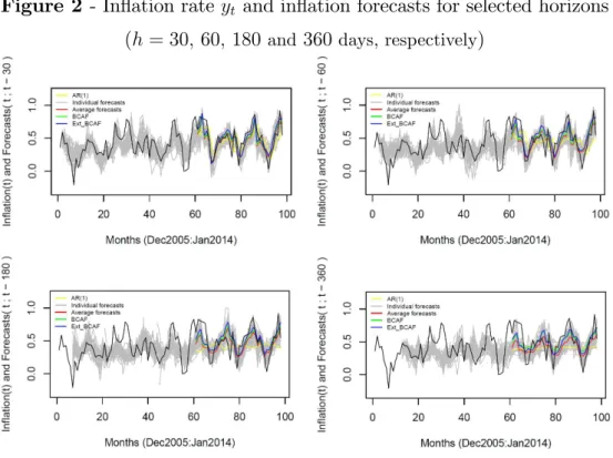
of 0:621 – estimated standard error of 0:068. Figure 2 plots monthly in‡ation and the respective daily forecast for survey respondents at horizons h = 30;60;180;360

days. It also presents the AR(1) forecasts, the average forecasts, the BCAF, and

the extended BCAF, at these same horizons.

Figure 1 - CPI in‡ation rate in Brazil (yt)

Monthly (left plot) and twelve-month (right plot) accumulated rates (%)

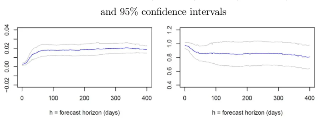
Table 1 reports GMM estimates for the extended BCAF. Although estimates of the average intercept are close to zero, and estimates of the average slope are close to unity, they are all highly signi…cantly di¤erent to zero at any given horizon.

A Wald-test for zero average intercept and unity average slope highly rejects the null at all horizons, showing the usefulness of the approach proposed in this paper. Figure 3 plots these two estimates across daily (working days) horizons with 95%

Figure 2 - In‡ation rate yt and in‡ation forecasts for selected horizons

(h= 30;60; 180 and 360 days, respectively)

Note: Yellow lines present the AR(1) forecasts. Gray lines show the forecastsf_i;th of survey participanti

foryt made at periodt h: Red lines represent the average forecast, and the green and blue lines show,

respectively, the BCAF and the Extended BCAF forecasts. Black line is the in‡ation ratey_t:

Table 1 - GMM estimation results

horizon h (days) kbh ch _{Wald test (p-value) OIR test (p-value)}

10 0:0036

(0:0009) 0(0::96380276) 1:1E 13 0:7059

20 0:0071

(0:0016) 0(0::93120399) 3:0E 12 0:7038

30 0:0118

(0:0026) 0(0::89290481) 7:5E 16 0:6237

60 0:0173

(0:0033) 0(0::85410583) 9:6E 11 0:6532

90 0:0180

(0:003) 0(0::86470763) 1:8E 12 0:7095

180 0:0176

(0:003) 0(0::84860884) 2:8E 11 0:6884

360 0:0199

(0:0025) 0(0:8275:088) 2:9E 15 0:5893

Note: Robust standard errors in parentheses. Wald test refers toHo: [kh; h] = [0; 1]:

Figure 3 - Estimates kbh _{(left panel) and}ch _{(right panel)}

and 95% con…dence intervals

We compare the out-of-sample MSE of each of the four forecast methods em-ployed here: the AF, the BCAF, the extended BCAF and the AR(1) model as well

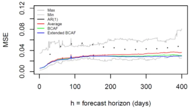
as the minimum and maximum MSEs across all survey respondents included in our sample. Figure 4 plots the daily results for these methods17_{. The …rst interesting}

feature is the comparison between the AR(1) model and the forecast-combination

techniques discussed here – the AF, the BCAF, and the extended BCAF. Strikingly, notice that the AR(1) model is usually close to upper bound of the MSE, while the …rst three methods are all close to the lower bound. This shows that forecast

combi-nation works in practice – in our case, the optimal combicombi-nation of survey forecasts. These are exactly the results obtained by Ang et al. (2007) and Faust and Wright (2013).

Next, when we compare the MSE of the four methods discussed above there is an obvious pecking order: the extended BCAF is superior to the BCAF, which in turn dominates the AF, which in turn dominates the AR(1) model. This validates the

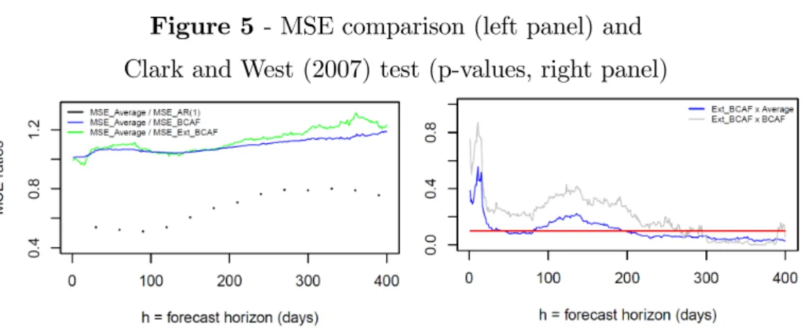
view that the bias corrections performed either by the BCAF, or by the extended BCAF, are a useful device for forecasting using surveys. As shown in Table 2 and Figure 5 (left panel), when we compare the extended BCAF, or the BCAF, with

the AF, forecasting MSE reductions can reach up to 25% at some horizons for the extended BCAF, and can reach up to 15% for the BCAF, although they are usually at the 10%-15% range. Reductions vis-à-vis the MSE associated with forecasts of

the AR(1) model for in‡ation can reach up to 50% for the extended BCAF.

Figure 4 - Mean Squared Error (MSE)

Note: Max (Min) denotes the maximum (minimum) MSE, for each horizon,

across all forecasters. Average refers to the MSE of the consensus forecast.

Table 2 - Mean Squared Error (MSE)

horizon h (days) AR(1) Average

Forecast BCAF

Extended

BCAF

30 0:0328

[0:000] 0(0:0177:105) 0(0:0166:247) 0:0164

60 0:0475

[0:001] 0:(00248:081) 0(0:0234:206) 0:0226

90 0:0523

[0:005] 0(0:0267:119) 0(0:0254:261) 0:0249 180 0:0466

[0:049] 0(0:0312:124) 0(0:0294:297) 0:0293 270 0:0415

[0:046] 0:(00328:056) 0:(00293:099) 0:0281 360 0:0452

[0:019] 0:(00357:028) 0:(00309:000) 0:0275

Notes: The second column shows [in brackets] the p-values of the equal variances’ test of Diebold-Mariano (1995)

between the AR(1) and the Extended BCAF. The third and fourth columns show (in parenthesis) the p-values

of the equal-predictive accuracy test of Clark and West (2007), which compares the Extended BCAF

and the forecast in each column. In all cases, * indicates a rejection of the null at a 10% level.

Finally, we test whether or not forecast errors di¤er in a statistical sense.

Fig-ure 5 (right panel) presents the equal-predictive-accuracy test of Clark and West (2007) for nested models at di¤erent horizons. Results suggest that, vis-à-vis the average forecast, both bias-correction devices (BCAF and the extended BCAF) can

statistically reduce (at the 10% signi…cance level) out-of-sample MSE for horizons above 9 months, and marginally reduce the MSE for h ranging between 1 and 3 months. The Clark-West test also indicates that the extended BCAF can

(h > 10 months). Comparisons of the extended BCAF with the AR(1) model us-ing a Diebold-Mariano test for equal variances shows that the former is statistically

superior to the latter (at the 10% signi…cance level) at all horizons.

Figure 5 - MSE comparison (left panel) and

Clark and West (2007) test (p-values, right panel)

Note: On the right panel, the red line represents a p-value of 0.10 and Ho: equal predictive accuracy.

4

Conclusion

In a world where there is an increasing availability of reliable data provided elec-tronically, it is interesting to examine how one could e¢ciently use this wealth of

information – big data. Our focus here is on the abundant information contained in expectation surveys that can now be built on thousands (or millions) of respondents on an almost continuous-time basis, and how it can be used e¢ciently for forecasting

purposes. We think of this problem as having two layers. In the …rst layer, there is the decision of survey respondents on what forecast should be supplied, consid-ering a given target variable of the survey. On the second layer, there is a user of

the survey who wants to forecast e¢ciently the target variable using all the survey information. We think of the latter as the econometrician.

For the decision in the …rst layer, we employ standard microeconomic and

econo-metric techniques to model the optimal survey response. Under suitable conditions that are standard in the literature, we show that the optimal forecast of a given survey respondent is an a¢ne function of the conditional expectation of the target

variable of the survey. Assuming that the …nal user of that information has a mean-squared-error (MSE) risk function, we show how to estimate the optimal forecast (conditional expectation) from the point-of-view of the econometrician. Our