Recursive Neuro Fuzzy Techniques for Online Identification and Control

(1)

Tiago Miguel Brites Oliveira

Licenciado em Engenharia Electrotécnica e de Computadores

Recursive Neuro Fuzzy Techniques for Online

Identification and Control

Dissertação para obtenção do Grau de Mestre em Engenharia Electrotécnica e de Computadores

Orientador :

Luís Filipe Figueira Brito Palma, Prof. Auxiliar,

FC-T/UNL

Co-orientador :

Paulo José Carrilho de Sousa Gil, Prof. Auxiliar,

FCT/UNL

Júri:

Presidente: Prof. Doutor Luís Filipe dos Santos Gomes - FCT/UNL Arguente: Prof. Doutor José António Barata de Oliveira - FCT/UNL

(2)

(3)

iii

Recursive Neuro Fuzzy Techniques for Online Identification and Control

Copyright cTiago Miguel Brites Oliveira, Faculdade de Ciências e Tecnologia, Univer-sidade Nova de Lisboa

(4)

(5)

(6)

(7)

Acknowledgements

Quero exprimir os meus agradecimentos ao orientador da tese Luís Palma e ao co-orientador Paulo Gil, pelo suporte e orientação a nível tanto técnico como teórico.

(8)

(9)

Abstract

The main goal of this thesis will be focused on developing an adaptative closed loop control solution, using fuzzy methodologies. A positive theoretical and experimental contribution, regarding modelling and control of fuzzy and neuro fuzzy systems, is ex-pected to be achieved.

Proposed non-linear identification solution will use for modelling and control, a recur-rent neuro fuzzy architecture. Regarding model solution, a state space approach will be considered during fuzzy consequent local models design. Developed controller will be based on model parameters, being expected not only a stable closed loop solution, but also a static error with convergence towards zero. Model and controller fuzzy subspaces, will be partitioned throughout process dynamical universe, allowing fuzzy local models and controllers commutation and aggregation.

With the aim of capturing process under control dynamics using a real time approach, the use of recursive optimization techniques are to be adopted. Such methods will be applied during parameter and state estimation, using a dual decoupled Kalman filter ex-tended with unscented transformation.

Two distinct processes one single-input (SISO) other multi-input (MIMO), will be used during experimentation. It is expected from experiments, a practical validation of pro-posed solution capabilities for control and identification. Presented work will not be completed, without first presenting a global analysis of adopted concepts and methods, describing new perspectives for future investigations.

Keywords: Recursive optimization, online identification, adaptative control, self

(10)

(11)

Resumo

O objectivo primordial desta tese tem por base o desenvolvimento de uma solução de controlo adaptativo fazendo uso de metodologias difusas. Consequentemente, pretende-se com esta dispretende-sertação dar um contributo positivo para modelos e controladores descri-tos segundo métodos difusos e neuro difusos.

A solução de controlo passa pela criação de um modelo não linear, baseado numa arqui-tetura neuro-difusa recorrente com modelos locais descritos sobre a forma de espaço de estados. É também desenvolvido um controlador neuro difuso recorrente, baseado nos parâmetros do modelo, que permita uma solução estável em anel fechado com um erro estático convergente para zero. Tem-se como objectivo a criação de um modelo distri-buído pelo universo de funcionamento do processo, permitindo a comutação e agregação de diversos modelos e controladores locais.

Procurando capturar as dinâmicas do processo sobre controlo, segundo uma abordagem em tempo real, é necessária a utilização de técnicas de optimização, com capacidades de recursividade. Para o efeito, recorre-se neste trabalho, a técnicas de estimação de parâ-metros e de estados baseadas no filtro de Kalman dual e desacoplado, estendido com a técnica de transformação de incerteza.

É efetuada uma análise experimental utilizando dois processos distintos, visando a conci-liação dos conceitos teóricos apresentados na solução proposta. Na experimentação serão demostradas as capacidades de identificação e controlo para sistemas não só de uma en-trada e uma saída (SISO), como também para sistemas de múltipla enen-trada múltipla saída (MIMO). Irá ser realizada uma análise global da solução, incluindo novos pontos de vista para caminhos de futuras investigações.

Palavras-chave: Estimação recursiva, identificação em linha, controlo adaptativo, auto

(12)

(13)

List of Figures

1.1 Global solution block diagram. . . 2

1.2 Closed loop identification block diagram . . . 3

1.3 Optimization algorithm block diagram. . . 4

2.1 Illustration of crisp and fuzzy sets . . . 11

2.2 Basic operations on fuzzy sets . . . 13

2.3 Fuzzy set with height= 1, support= [0,0.8]and core= [0.4,0.6] . . . 14

2.4 Convexity of a fuzzy set . . . 14

2.5 Intersection and union operators . . . 17

2.6 Complement operators. . . 18

2.7 Different shapes of MFs a) MF-DSIG; b) MF-G;c)MF-SIG;d) MF-SG; e) MF-PI;f)MF-PSIG;g)MF-Z;h)MF-TRI;i)MF-TRAP; . . . 22

2.8 Fuzzy inference block diagram . . . 23

2.9 A fuzzy example using Mandani inference . . . 26

2.10 A fuzzy example using Mandani inference for a TS system and a standard fuzzy system . . . 26

3.1 Blackbox modelling problem . . . 31

3.2 Block schema of an NARX structure fora)series-parallel identificationb) series identification . . . 33

3.3 Block schema of a State Space representation . . . 36

3.4 A neuronjin layerr . . . 39

3.5 A feedforward neural network . . . 39

3.6 Simplified flexible neuro-fuzzy using mandani inference . . . 41

3.7 A flexible ANFIS structure . . . 42

3.8 Proposed RNFS network with a state-space rule base . . . 46

3.9 Proposed series-parallel RNFS network . . . 46

3.10 Proposed series RNFS network . . . 47

(18)

xviii LIST OF FIGURES

3.12 Proposed closed loop architecture,_Wkˆ _{is the model parameters,} _WˆK

k and

ˆ

WR

k are controller parameters . . . 51

5.1 Workflows for system identification and control . . . 82

5.2 Feedback PT 326 plant . . . 85

5.3 PT326 Collected data . . . 86

5.4 RNFMS membership functions . . . 87

5.5 RNFMS with rules consequents optimized,WCdivergence phenomenon. 88 5.6 RNFMS with rules consequents optimized, no divergence. . . 89

5.7 RNFMS with rules consequents and states optimized,M SE: ˆySP _{= 1}_.₄₈₃₄_e−4_{; ˆ}_yP ₌ 1.5641e−4; ˆy= 1.3318e−5 . . . 90

5.8 RNFMS with rules consequents, states and MFs optimized,M SE : ˆySP ₌ 1.5297e−4; ˆyP _{= 1}_.₅₄₈₉_e−4_{; ˆ}_y_{= 1}_.₃₅₉₁_e−5 _{. . . .} ₉₁

5.9 Fis model dynamics. . . 93

5.10 RNFMS dynamics for fis model . . . 93

5.11 Controller initialization (reference in RNFCS premise) . . . 94

5.12 Closed loop real-time experiments (reference in RNFCS premise) . . . 95

5.13 Closed loop real-time experiments using covariance reset (reference in RN-FCS premise). . . 96

5.14 Amira DTS200 plant . . . 97

5.15 Data for offline identification . . . 98

5.16 Default local model response . . . 100

5.17 RNFMS response with optimized consequents . . . 101

5.18 RNFMS response with optimized consequents and states . . . 102

5.19 RNFMS response with optimized consequents, states and MFs, using all plant sensors . . . 103

5.20 RNFMS response with optimized consequents, states and MFs, without using sensor T3 . . . 104

5.21 Offline local controller optimization . . . 106

5.22 RNFCS with controller in premise, tank three and RNFMS with MF opti-mization (Exp.1) . . . 107

5.23 Online RNFMS and RNFCM gain evolution. RNFCS with controller in premise, tank three and RNFMS with MF optimization (Exp.1) . . . 108

5.24 RNFCS with controller in premise, tank three and RNFMS without MF optimization (Exp.2) . . . 109

5.25 Online RNFMS and RNFCS gain evolution. RNFCS with controller in premise, tank three and RNFMS without MF optimization (Exp.2) . . . 110

5.26 Experimental results comparison . . . 111

(19)

LIST OF FIGURES xix

5.28 Online closed loop response with plant failures. RNFCS with reference in

premise, no tank three and RNFMS without MF optimization . . . 113

B.1 2-state CSTR simulation using standard UKF,α= 1 . . . 138

B.2 2-state CSTR simulation using PUKF,α= 1 . . . 139

B.3 2-state CSTR simulation using CIUKF,α= 1 . . . 140

B.4 2-state CSTR simulation using standard UKF,α= 0.1 . . . 141

B.5 2-state CSTR simulation using PUKF,α= 0.1 . . . 142

B.6 2-state CSTR simulation using CIUKF,α= 0.1 . . . 143

B.7 2-state CSTR simulation using CIUKF,α = 0.9,λr = 0,λe = 0,Rr 0 = 0.1 andRe₀ = 1 . . . 144

B.8 2-state CSTR simulation using IUKF, α = 0.9,λr = 0,λe = 0.2,Rr 0 = 0.1 andRe 0 = 1 . . . 145

B.9 2-state CSTR simulation using IUKF, α = 0.9,λr = 0.2,λe = 0,Rr₀ = 0.1 andRe 0 = 1 . . . 146

(20)

(21)

List of Tables

4.1 UKF state estimation for additive noise case (system as Equation 4.14) . . 64

4.2 UKF for parameter estimation considering additive noise case. (system as in Equation 4.14) . . . 65

4.3 Formulation of ICUT . . . 68

5.1 PT326 input data script . . . 86

A.1 RNFMS decoupled UKF consequents parameter estimation considering additive noise case. (system as in Equation 4.16) . . . 127

A.2 RNFMS decoupled CIUKF membership parameter optimization consider-ing additive noise case. (system as in Equation 4.16) . . . 128

A.3 RNFMS decoupled CIUKF rules and inputs degree optimization consider-ing additive noise case. (system as in Equation 4.16) . . . 130

A.4 RNFMS decoupled UKF state estimation considering additive noise case. (system as in Equation 4.16) . . . 132

(22)

(23)

Acronym List

ANFIS - Adaptative-Network-Based Fuzzy Inference System ARX - Autoregressive with Exogenous inputs

COA - Center of Area Defuzzification EKF - Extended Kalman Filter

FIS - Fuzzy Inference System FS - Fuzzy System

FSS - Fuzzy State-Space GA - Genetic Algoritm

ICUKF - Interval Constrained Unscented Kalman Filter ICUT - Interval constrained Unscented Transformation IUKF - Interval UKF

KF - Kalman Filter

MBC - Model Based Controller MF - Membership Function MSE - Mean Square Error

MRAFC - Model Reference Adaptative Fuzzy Control NFM - neuro fuzzy modeling

NFS - Neuro Fuzzy System

pdf - Probability Density Function

PSO - Particle Swarm Optimization Algorithm PUKF - Projected UKF

RNF - Recursive Neuro Fuzzy

(24)

xxiv Acronym List

SSNFS - State Space Neuro Fuzzy System SUT- Scaled Unscented Transformation TIUKF - Truncated Interval UKF TSK - Takagi-Sugeno and Kang TUKF - Truncated UKF

UD - Universe of Discourse UKF - Unscented Kalman Filter

UPUKF - Unconstrained Projected UKF

URNDDR - Unscented Recursive Nonlinear Dynamic data Reconciliation UT- Unscented Transformation

WAM - Weighted Average Method Defuzzification

Rr

(25)

1

Introduction

1.1 Global motivations

(26)

1. INTRODUCTION 1.2. Goals and contributions

optimum solutions.

1.2 Goals and contributions

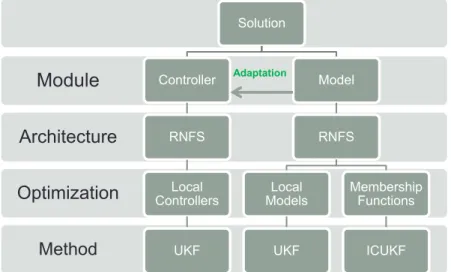
Having in scope a model and controller design defined by several local models and con-trollers, two major theories have been selected i.e fuzzy modelling and neural networks. Combining both methods into a single concept, will result in a new theory known in lit-erature by neuro fuzzy modelling (NFM). This new method for system modelling, takes the advantage of fuzzy by allowing a continuous and stable model switching during real-time evaluation. By making use of neuro networks, NFM diminishes fuzzy infer-ence process abstractness. It also allows an augmentation of fuzzy model parameters, due to creation of weights between neuron connections. Several neuro fuzzy systems (NFS) architectures were already developed and analysed. Although, most of them use an ARX structure for model design (case of ANFIS structure), being difficult to directly implement a MBC controller using system states. Some proposals for NFS using local models structured in a state space approach exist in literature, but none featured with recursiveness. Due to adaptation requirements, learning algorithm should be able to be computed during real-time processing, fulfilling process sampling times. Among sev-eral algorithms which fits into this class, a Kalman filtering (KF) technique was adopted due to its recursive nature. An extension to standard KF method known as Unscented Transformation (UT) was considered, allowing to compute model mean and covariance in a statistical fashion. The extension of KF with UT, is known in literature by Unscented Kalman Filtering (UKF), where instead of finding a model that best fits process output dynamics, it will fit model to process output distribution. Proposed global solution for system identification and control, is described inFigure 1.1.

Method

Optimization

Architecture

Module

Solution

Controller

RNFS

Local Controllers

UKF

Model

RNFS

Local Models

UKF

Membership Functions

ICUKF

Adaptation

Figure 1.1: Global solution block diagram

(27)

noticed two modules were defined, a controller and a model. For both, a new Recursive Neuro Fuzzy architecture (RNF), using state space local models and controllers, was de-veloped. Both modules will be under a real time recursive optimization, handled by UKF algorithm. Model will not only enforce optimization in rules local models, both for states and parameters, but also in membership functions (MF). Controller in opposition, will not handle MF optimization because it will use model premises. A constrained prob-lem must be considered during MF optimization, which was addressed by other UKF extension known as Interval Constrained Unscented Kalman Filter (IUKF). Optimization of Rules aggregation and input weights is also seen as a constrained problem, although experimentation will not handle such optimization. New scientific contributions can be found in settled goals, precisely a new RNFS architecture which can be used both for controller and model design. Also, a new integration and applicability of UKF and IUKF theory was achieved, by applying it to a RNFS model and controller optimization.

(1) Identification of non-linear systems

The new NFS topology (as so far observed) proposed in this work, is featured with recurrence capabilities and contains eight layers handling fuzzification, fuzzy infer-ence and defuzzification. The number of neurons for each layer depends on input and output variables, number of states and membership functions. The number of MFs depends on adopted fuzzy partitions, which should reflect process working zones. Increasing fuzzy partitions, might also increase model accurateness if enough input data is used to stimulate process throughout its working points. Although, it is also expected an augmentation of model and controller complexity, since new rules need to be considered. Complete process identification will be handled in a closed loop control solution as described inFigure 1.2.

 Controller

RNFS Plant

Model RNFS UKF

u

y

ˆ

e



d

y

UKF\ICUKF

x

ˆ

C



ˆ

 



ˆ

,

 



ˆ

,





e

Figure 1.2: Closed loop identification block diagram

(28)

consequently, an improvement of prediction accuracy. An analytical study regarding stability analysis will not be presented, its is known that local models might suffer from zero pole cancellation and become unstable and uncontrollable. For a better un-derstanding ofFigure 1.2, it is worth a brief description regarding involved variables, which will be introduced insection 4.4. It should be considered:

• ydis the desired process output values;

• xˆstands for model predicted states;

• ωˆC _{is the RNFS local controllers predicted parameters;}

• ωˆµ;ψ _{is the prediction of RNFS local models membership functions and}

conse-quents respectively;

• yis the process output;

• yˆis the model predicted output;

• eandηare additive Gaussian noise for parameters and outputs respectivelly.

(2) Recurrent algorithm for training neuro fuzzy systems

Regarding the use of UKF algorithm for RNFS identification, a sequential approach as defined inFigure 1.3was considered.

C

UKF s Con sequ en t

Pr ed i cti on Con tr oll er

 

UKF

s Consequ en t

Pr ed i cti on Mod el k y  k xˆ  1 ˆ_k x  k xˆ    ˆk 1



 ˆ_k 

 ˆ_k



 ˆ_k



 ˆ_k

 

 ˆk 1

k

y

k

y C

UKF_ Up d ate t Measur emen  C k ˆ  C k ˆ   C k 1 ˆ  d k

y 1

 

UKF

Fu n ti on s Member sh i p

Pr edi cti on Mod el

 

UKF

Up d ate t Measur emen x UKF Update t Measur emen x UKF Predi cti on State

 

UKF

Up d ate t Measur emen

Figure 1.3: Optimization algorithm block diagram

(29)

1. INTRODUCTION 1.3. Thesis structure

to produce the next most accurate control action. It is worth mention that controller innovations, depend on error between output and reference. Regarding model, its innovations will use as cost factor the error between predicted and process outputs. Due to KF nature, it is expected for both errors a convergence to zero.Figure 1.3 vari-ables will be introduced inchapter 4meanwhile, a brief description for a better figure understanding should be handled. It is defined:

• xˆ+_k₋₁is the previous UKF prediction of model state;

• xˆ−_k is the current UKF prediction of model state after algorithm time update

stage;

• xˆ+_k is the current UKF prediction of model state; • ykcurrent process output;

• yd

k+1is the next process output desired values;

• ωˆ_kψ₋+₁is the previous UKF prediction for RNFS model consequents parameters; • ωˆ_kψ−is the current UKF prediction for RNFS model consequents parameters after

algorithm time update stage;

• ωˆ_kψ+is the current UKF prediction for RNFS model consequents parameters; • ωˆ_kµ₋+₁is the previous UKF prediction for RNFS model membership functions; • ωˆ_kµ− is the current UKF prediction for RNFS model membership functions after

algorithm time update stage;

• ωˆ_kµ+is the current UKF prediction for RNFS model membership functions;

• ωˆ_kC₋+₁is the previous UKF prediction for RNFS controller parameters;

• ωˆ_kC− is the current UKF prediction for RNFS controller parameters after algo-rithm time update stage;

• ωˆ_kC+is the current UKF prediction for RNFS controller parameters;

• U KFxUKF algorithm for RNFS model state optimization;

• U KFωψUKF algorithm for RNFS model consequents parameter optimization; • U KFωµUKF algorithm for RNFS model membership functions optimization

(us-ing ICUKF extension);

• U KFC

ω UKF algorithm for RNFS controller parameter optimization

1.3 Thesis structure

(30)

describing what remains to be done, future enhancements and other capabilities and applications beyond used ones.

Chapter 2: Fuzzy Logic Systems: Theory and Concepts

This chapter introduces a brief overview regarding fuzzy notions. It starts with a description about fuzzy sets and their operations, finishing with a description of fuzzy inference mechanisms.

Chapter 3: Fuzzy System Modelling

Focusing on model design phase, several modelling methodologies will be pre-sented. Chapter starts with an overview regarding ARX, NARX and state space model structuring. Then it continues with a description of neuro networks con-cepts and their evolution to neuro fuzzy networks. Chapter ends with a new net-work structuring proposal, which can be seen as an upgrade over existing state of the art methods. Also a complete closed loop network solution as in Figure 1.2

regarding process identification and control is presented.

Chapter 4: Estimation Methods for Fuzzy Structures Parameters

This chapter provides the next step towards final system identification solution. It starts with an introduction of Kalman statistical properties and the principle of unscented transformation. Also the pervasive computation of UKF regarding state and parameter optimization is demonstrated. Searching for a better comprehension regarding UKF and RNFS integration, chapter includes an analytical description of RNFS architecture parameters, comprising variable design and dimensioning both for controller and model. Having defined RNFS variables, chapter describes the computation of ICUKF and UKF for RNFS optimization. For a better understand-ing of UKF intrinsic variables and dynamics, a theoretical model well known in literature, will serve as use case for a better understanding regarding algorithm convergence and stability.

Chapter 5: Implementation

(31)

Chapter 6: Global Conclusions and Further Research

(32)

(33)

2

Fuzzy Logic Systems: Theory and

Concepts.

2.1 Introduction

This chapter aims to introduce fundamental notions regarding fuzzy reasoning. Pre-sented theory will allow a complete understanding of proposed solution. Firstly, it will handle basic notions regarding fuzzy sets and their evolution from crisp sets. Having introduced fuzzy sets, it will continue with an analytical description of standard oper-ations on fuzzy sets including their shapes known as MFs. Before starting with fuzzy inference process, it is worth defining fuzzy relations, since it contains key aspects for understanding of fuzzification, implication and defuzzification processes.

2.2 Fuzzy sets theory.

(34)

2. FUZZYLOGICSYSTEMS: THEORY ANDCONCEPTS. 2.2. Fuzzy sets theory.

2.2.1 Classic sets.

For more information regarding classic sets consider [1], since presented work will only demonstrate key notions, which will be used as starting point for the introduction of fuzzy sets. Classic or crisp sets are all sets whose elements have only two states i.e, it can either full belong or not belong to a set. Take as example the boolean logic where a vari-able can only be zero or one. LetUbe a not empty set also known asuniverse of discourse (UD), it contains all possible elements or members of a given context, each of those ele-ments are contained inU. The union of several elements ofUis known as a subsetUofU.

Definitions:

• u_∈U - a memberuofUbelongs to the subsetU ofU;

• u /_∈U -uis not member ofU;

• u⊆U-U is subset ofUorU iqualU;

• ∅- empty set;

Sets with distinct properties P1...Pn for all UD are assigned with a linguistic term for

instanceAwhere:

A=_{a_|awith propertiesP1...Pn}

Each set properties can be described by their characteristic function, defined as::

fA= (

1, ifu_∈A

0, ifu /_∈A (2.1)

In other words, characteristic function performs the mapping of elements contained in

U to elements in domain {0,1_} by using fA : U → {0,1}. If fA(u) = 1, u ∈ A

oth-erwise, if fA(u) = 0, u /∈ A. The characteristic function of a subset of U, where

sub-set U is the aggregation of all n sets ∈ U, is defined as f(u), and is the projection of

fA1(u), fA2(u), ..., fAn(u),withn∈ ℜalongy−axis∀u∈U.

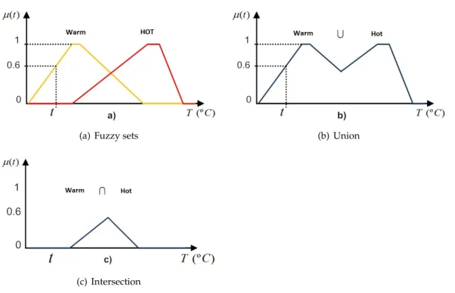
Figure2.1(a)displays the characteristic function of two crisp sets, with linguistic words “Warm” and “Hot”, where Ucovers the temperature (T) value range of a roomT _{∈ ℜ}. In many cases U ∈ ℜn _{belongs to a range}_∈ _[₋₁_,_1]_{, becoming in this case known as}

“normalized universe of discourse”.

2.2.2 Fuzzy sets.

(35)

(a) Crisp sets (b) Fuzzy sets

Figure 2.1: Illustration of crisp and fuzzy sets

union. For a profound theoretical analysis it is highlighted [3].

As it can be seen through2.1, the main disadvantage of a crisp against a fuzzy set, dues to a constrained linguistic variable u ∈ ℜcharacteristic function, supporting only two values. Concerning given example, the room temperatures will vary abruptly from a full ”Warm” to a full ”Hot” state. It was towards this direction that fuzzy sets evolved, al-lowing a characteristic function with a smooth transition between sets as it can be seen by2.1(b). Fuzzy sets can be seen as an extension of crisp sets, where instead of mapping a fuzzy variable into set of values _{0,1_}, it maps to a value contained in interval[0,1].

The characteristic function of a fuzzy set can be defined as:

fA:U→[0,1]∈ ℜ or

µA:U→[0,1]∈ ℜ

(2.2)

whereµAis the membership function of a fuzzy set A whose value represents the

vari-ableu∈Udegree of membership on set A. For instance, through2.1(b)it can be noticed

that linguistic variable t _∈ T (where T is the UD), contains a degree of membership µW arm(t) = 0.6in set “Warm” andµHot(t) = 0set “Hot”. Next will be presented several

definitions from the standard fuzzy sets theory (SFST):

Definition (Fuzzy Set)- A fuzzy set defined in spaceUis a set of pairs:

A=_{(u, µA(u)), u∈U}, ∀x∈U. (2.3)

Definition (Empty)- A fuzzy setAis called empty if:

∀u∈U,µA(u) = 0. (2.4)

Definition (Equality)- Two fuzzy setsAandBare equal if:

(36)

Definition (Complement)- A fuzzy setAcomplement denoted byA′_{is defined as:}

µ_A= 1−µA. (2.6)

Definition (Containment)-Ais contained inB, orAis a subset ofB, if:

µA⊂µB ⇐⇒A≤B. (2.7)

Definition (Union)- Union of two fuzzy setsAandBwith respective membership

func-tionsµAandµB is a new fuzzy setC whereC =A∪B, whose membership function is

related toµAandµBthrough:

µC(u) =M ax[µA(u), µB(u)] ∀u∈U (2.8)

or simply

µC =µA∨µB. (2.9)

In other words, the union ofAandBis the lowest fuzzy set containingAandBa s it can be seen by2.2(b).

Definition (intersection)- Intersection of two fuzzy setsAandBwith membership func-tionsµAandµBrespectively, is a new fuzzy setCsuch thatC =A∩B, where its

mem-bership function is related withµAandµBthrough:

µC(u) =M in[µA(u), µB(u)] ∀u∈U (2.10)

or simply

µC =µA∨µB. (2.11)

In other words, intersection ofAandB is the highest fuzzy set which is contained inA

andB, as it can be observed from2.2(c). It is worth mention that for fuzzy sets, in opposi-tion to crisp sets, is has no meaning saying that a given linguistic variable belongs to a set ifµA(u)>0with u∈ U. In fuzzy domain multiple intervals can be defined for instance, α andβ with, 0 < α < 1; 0< β < 1andβ < α. Also, sentence “ubelongs to A” might depend on several constraints, for instance if µA(u) > α orβ < µA(u) < α. Fuzzy sets

are not constrained to a single value logic, they allow reasoning based on a multi value logic.

Definition (Height) - The height of a fuzzy set A is the maximum value of its

mem-bership function:

hgt(A) =sup u∈U

µA(u). (2.12)

(37)

(a) Fuzzy sets (b) Union

(c) Intersection

Figure 2.2: Basic operations on fuzzy sets

Definition (Support)- Support of a fuzzy set A corresponds to all values ofu _∈ Uover

whichµA(u)>0, this means:

supp(A) =_{u_∈U|µA(u)>0}. (2.13)

Definition (Core)- Core of a fuzzy set A corresponds to all values ofu ∈Uover which µA(u) = 1i.e:

core(A) =_{u_∈U|µA(u) = 0}. (2.14)

A fuzzy set A is normal if its core is not empty. 2.3demonstrates a use case of concepts “height”,“core”,“support” of a fuzzy set having linguistic word “Warm”.

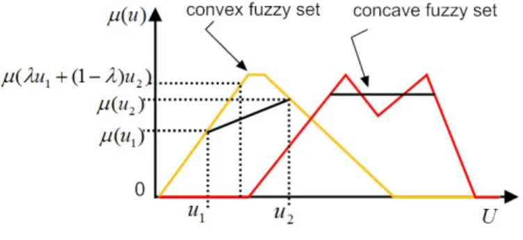
Definition (Convexity)- A fuzzy set A is convex if for anyu1, u2 ∈Ungivenλ∈[0,1]

µA(λu1+ (1−λ)u2)≥min{µA(u1), µA(u1)}. (2.15)

as shown in2.4.

Definition (Symmetry) - A fuzzy set is symmetric if its membership function is

sym-metric around a given pointc

(38)

Figure 2.3: Fuzzy set with height= 1, support= [0,0.8]and core= [0.4,0.6]

Figure 2.4: Convexity of a fuzzy set

2.2.3 Triangular norms and negation.

Several studies in the field of fuzzy set theories have been done [2] (pp. 30-63) although, section2.2.2only introduced classic theory from Zadeh. This section presents other the-ories as t-norm, t-conorm and negation, which mathematical nomenclature is based on [4](pag. 13-21).

Definition (t-norm)- The t-norm is a functionT of two variables

T : [0,1]×[0,1]→[0,1] (2.17)

satisfying conditions:

1. T is monotonous

T{µA(u), µC(u)} ≤T{µB(u), µD(u)} ∀µA(u)≤µB(u)eµC(u)≤µD(u) (2.18)

2. T is commutative

(39)

3. T is associative

T{T{µA(u), µB(u)}, µC(u)}=T{µA(u), T{µB(u), µC(u)}}, (2.20)

4. T satisfying boundary conditions

T{µA(u),0}= 0,T{µA(u),1}=µA(u), (2.21)

withµA(u), µB(u), µC(u), µD(u) ∈[0,1] ∧ u∈U.

symbolically, t-norm in arguments µA(u), µB(u) refers to the intersection of two fuzzy

setsA, B_∈ Uwith membership functionsµAeµBrespectively,

T{µA(u), µB(u)}=µA(u) T

∗µB(u). (2.22)

µA∩B =µA(u) T

∗µB(u) (2.23)

Extending t-norm aggregation definition (2.20) ton >2variables

Tin=1{µAi}=T

Tin=1−1{µAi(u)}, µAn(u) =T{µA1(u), µA2(u), ..., µAn(u)}=

=T_{µ_A(u)_}=µA1(u)∗

T_µ A2(u)∗

T_..._∗T_µ An(u).

(2.24)

Definition (t-conorm)- T-conorm is a functionSof two variables

S: [0,1]_×[0,1]_→[0,1] (2.25)

satisfying conditions:

1. Sis monotonous

S_{µA(u), µC(u)} ≤T{µB(u), µD(u)} ∀µA(u)≤µB(u)eµC(u)≤µD(u), (2.26)

2. Sis commutative

S_{µA(u), µB(u)}=S{µB(u), µA(u)}, (2.27)

3. Sis associative

S_{S_{µA(u), µB(u)}, µC(u)}=S{µA(u), S{µB(u), µC(u)}}, (2.28)

4. Ssatisfies boundary conditions

(40)

withµA(u), µB(u), µC(u), µD(u)∈[0,1] ∧ u∈U.

symbolically, t-conorm in argumentsµA(u), µB(u)is the union of two fuzzy setsA,B ∈U

with membership functionsµAandµBrespectively, and is defined as:

S{µA(u), µB(u)}=µA(u) S

∗µB(u). (2.30)

µA∪B =µA(u) S

∗µB(u) (2.31)

Extending t-conorm definition (2.28) ton >2variables

Sin=1{µAi(u)}=S

Sin=1−1{µAi(u)}, µAn(u) =S{µA1(u), µA2(u), ..., µAn(u)}=

=S_{µ_A(u)_}=µA1(u)∗

S_µ A2(u)∗

S_..._∗S_µ An(u).

(2.32)

Both t-norm and t-conorm have three general derivations:

• The family min/max already introduced in2.2.2defined as:

TM{µA1(u), µA2(u)}= min{µA1(u), µA2(u)}

SM{µA1(u), µA2(u)}= max{µA1(u), µA2(u)}

TM{µA1(u), µA2(u), ..., µA2(u)}= mini=1,...,n{µAi(u)}

SM{µA1(u), µA2(u), ..., µA2(u)}= maxi=1,...,n{µAi(u)}

(2.33)

• The family of algebraic triangular norms defined as:

TP {µA1, µA2}=µA1µA2

SP {µA1, µA2}=µA1 +µA2 −µA1µA2

TP{µA1, µA2, ..., µAn}=

Qn i=1µAi

SP{µA1, µA2, ..., µAn}= 1−

Qn

i=1(1−µAi)

(2.34)

TP also known as t-norm product, such asSP also known as t-conorm probabilistic

sum.

• Lukasiewicz triangular norm family are defined as:

TL{µA1, µA2}= max{µA1 +µA2−1,0}

SL{µA1, µA2}= min{µA1 +µA21,1}

TL{µA1, µA2, ..., µAn}= max{

Pn

i=1µAi−(n−1),0}

SL{µA1, µA2, ..., µAn}= min{

Pn

i=1µAi,}

(2.35)

Definition (negation)

1. A non increasing function N : [0,1] _→ [0,1] is called negation if N(0) = 1and

(41)

) ( )

(u _B u

S A    U ) ( )

(u B u

T

A 

 

U

(a) Intersection and union operators using min/max method

) ( )

(u B u

T

A 

  ₍_u₎ ₍_u₎

B S

A 

 

U U

(b) Intersection and union operators using algebric method

) ( )

(u _B u

T

A 

  (u) _B(u)

S

A 

 

U U

(c) Intersection and union operators using Lukasiewicz method

Figure 2.5: Intersection and union operators

2. A negation N : [0,1] → [0,1]is called strict negationN is continuous and strictly

decreasing.

3. A strict negationN : [0,1]_→[0,1]is called strong negation if it is an involution, in other words, ifN(N(µA(u))) =µA(u)

Simbolically a negation or complement of two fuzzy setsA, B∈ Uwith respective

mem-bership functionsµAandµBcan be written as

µ_A(u) =N(µA(u)) (2.36)

whereN(µA(u))can be any type of negation. In general, three types of negation can be

defined:

• Zadeh’s negation defined as

(42)

• Yager’s negation defined as

N(µA(u)) = (1−µA(u)p)

1

p_{, p >}₀ (2.38)

• Sugeno’s negation defined as

N(µA(u)) =

1₋µA(u) 1 +pµA(u)

, p >−1 (2.39)

2.6illustrates an example of three negations types, and2.5(a),2.5(b),2.5(c)demonstrates three types of intersection and union.

(a) Zadeh’s negation (b) Yager’s negation

(c) Sugeno’s negation

Figure 2.6: Complement operators.

2.2.4 Fuzzy Relations

This part describes the basic concepts of fuzzy relations used in fuzzy reasoning, which will be addressed during next section. The Cartesian product [4] is defined as:

Definition (Cartesian product) - Having two fuzzy sets A ⊆ U and _B _⊆ Y, then

the Cartesian product betweenAandBis denoted byA _× Band defined as:

µA×B(u, y) =min{µA(u), µB(u)}

or

µA×B(u, y) =µA(u).µB(u)

(2.40)

whereu ∈ U and_y _∈ Y are linguistic variables. For_nfuzzy sets_A₁ _⊆ U1, A₂ ⊆

(43)

as:

µA1×A2×...×An(u1, u2, . . . , un) = min

i=1...n{µAi(ui)}

or

µA1×A2×...×An(u1, u2, . . . , un) =

n Y

i=1

µAi(ui)

(2.41)

In a generic concept, the Cartesian product is described by a t-norm not being restricted to themin operator. A Fuzzy relation µR(u, y) is a mapping from the Cartesian space U _× Y to the interval[0 1][5] such that:

A_×B =R _⊂ U _×Y

= X

U×Y

µR(U×Y) (U_×Y₎

(2.42)

with membership function

µR(u, y) =µA×B(u, y)

= minµA(u), µB(y)

(2.43)

The Cartesian product defined in (2.42) is implemented through the cross product of two vectors, for instance consider fuzzy set

A= 0.2

u1

+ 0.6

u2

+ 1

u3

and fuzzy set

B= 0.3

y1

+0.9

y2

µRis computed through:

µR=

min(0.2,0.3)

u1, y1

+min(0.2,0.9)

u2, y2

+. . .+min(1,0.9)

u3, y2

relationRaccording to (2.42) can be expressed in matrix form:

A_×B =R=

y1 y2

u1 u2 u3   

0.2 0.3 0.3

0.2 0.6 0.9



 

Definition (Fuzzy composition)- Consider fuzzy relations R andS defined inU _×Y

(44)

byR_◦S _⊆U _×Zdefined as:

µR◦S(u, z) = sup y∈Y

µR(u, y)∗T µS(y, z) (2.44)

Fuzzy composition can also be applied to obtain a fuzzy setB_⊆Y from the composition

of fuzzy setA⊆U and fuzzy relation_R_⊆U_×Y this means,

B =A_◦R _⊆ Y

with membership function

µB(y) =µA◦R(y)

= sup u∈U

µA(u)∗T µR(u, y)

(2.45)

from above deductions∗T _{is a T-norm previously defined.}

2.2.5 Membership functions

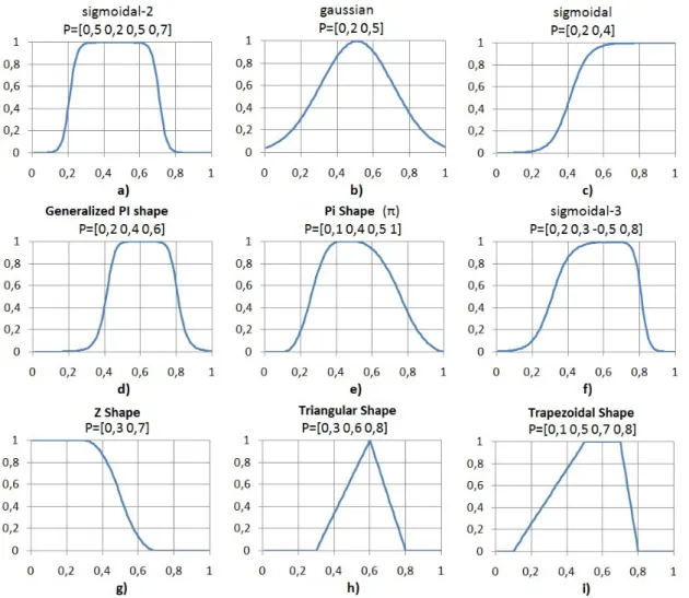
This section will introduce most common types of membership functions (MFs), which analytical definition can be found in [6]. As it was already mentioned in section2.2.2by

2.2, a MF of setArespectivelyµA, does a mapping of a fuzzy variable u ∈ Uthrough

fuzzy setA_∈ U, whereUis the UD defining the variable membership degree.

1. Gaussian MF “MF-G” (figure2.7b)), has three parametersσandc_{∈ ℜ}such that

f(u;σ, c) =e−(u2σ−2c)2 (2.46)

2. Generalized bell MF “MF-SG” (figure2.7d)), has three parametersa,b,c_{∈ ℜ}such

that

f(u;a, b, c) = 1

1 +_|u−_ac_|2b (2.47)

3. S-shaped MF “MF-S” (much similar with figure2.7c)), contains two parametersa

andb_{∈ ℜ}

f(u;a, b) =             

0, u≤a

2u_b−₋_aa2, a_≤u_≤ a+₂b

1₋2u−a b−a

2 , a+b

2 ≤u≤b

1, u_≥b

(2.48)

4. Sigmoidal shape MF “MF-SIG” (figure2.7c)), contains two parametersaandb_{∈ ℜ}

such that

f(u;a, b) = 1

1 +e−a(u−c) (2.49)

(45)

on this MF-SIG, two other functions can be defined through the product of two sig-moidal functions MF-SIG_×MF-SIG=MF-PSIG (figure2.7f)) or by their difference

MF-SIG−MF-SIG=MF-DSIG (figure2.7a))

5. Z-shaped MF “FP-Z” (figure2.7g)), contains two parametersaandb∈ ℜ

f(u;a, b) =             

1, u_≤a

1₋2u_b₋−_aa2, a_≤u_≤ a+₂b

2b− u b−a

2

, a+₂b ≤u≤b

0, u_≥b

(2.50)

6. Triangular shaped MF “MF-TRI” (figure2.7h)), contains three parametersa,band c_{∈ ℜ}

f(u;a, b, c) =           

0, u_≤a u−a

b−a, a≤u≤b c−u

c−b, b≤u≤c 0, c≤u

(2.51)

or in a compact form

f(u;a, b, c) = max

min

u₋a b₋a,

c₋u c₋b

,0

(2.52)

7. Trapezoidal shape MF “MF-TRAP” (figure 2.7i)), contains four parameters a, b, c

andd_{∈ ℜ}

f(u;a, b, c, d) =               

0, u≤a u−a

b−a, a≤u≤b 1, b_≤u_≤c d−u

d−c, c≤u≤d 0, d_≤u

(2.53)

8. PI(π) shaped MF “MF-PI” (figure2.7e)), contains four parametersa,b,candd∈ ℜ. This MF is built from the product between MF-S×MF-Z = MF-PI:

f(u;a, b, c, d) =                               

0, u_≤a

2u_b₋−_aa2, a≤u≤ a+b

2

1₋2u_b₋−_ab2, a+₂b _≤u_≤b

1, b≤u≤c

1₋2u_d₋−_cc2, c_≤u_≤ c+₂d

2u−d d−c

2

, c+d

2 ≤u≤d

0, u_≥d

(46)

2. FUZZYLOGICSYSTEMS: THEORY ANDCONCEPTS. 2.3. Fuzzy Inference

Figure 2.7: Different shapes of MFsa)MF-DSIG;b)MF-G;c)MF-SIG;d)MF-SG;e)MF-PI; f)MF-PSIG;g)MF-Z;h)MF-TRI;i)MF-TRAP;

2.3 Fuzzy Inference

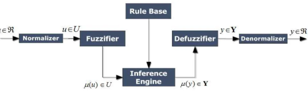
Any fuzzy system can be comprised by four main components Figure 2.8, a Fuzzifier, Defuzzifier, Inference Engine and a rule base, independently from the used inference type. Every fuzzy system should have a finite universe of discourse Uin order to be

practically conceivable. A finite UD is achieved through a normalizer and a denormalizer layers. The normalizer projects any input linguistic variableuontoUby a scaling factor

ˆ

u = u_k k _{∈ ℜ}. In opposition, the denormalizer undoes the initial projection by the same scaling factoru= ˆu×k k∈ ℜ.

2.3.1 Fuzzifier

This layer retains all information about fuzzy sets and their characteristic shapes i.e mem-bership functions. The fuzzifier firstly takes as input a crisp variableu _{∈ ℜ}n, then

(47)

Figure 2.8: Fuzzy inference block diagram

which is a normalized UD_∈ [₋1,1]. Fuzzifier also assignsuwith a grade of

member-ship in all fuzzy sets defined inU[7](pp.49-51). This degree of membership can be seen

as a vector whose elements are membership grades per each linguistic value. The map is defined according to (2.2). Analytically the fuzzifier computes:

µ_A

i(ui) =

" TnµA′

i(ui), µA1i(ui)

o

TnµA′

i(ui), µA2i(ui)

o

. . . T (

µA′

i(ui), µ

Ani_imf (ui)

)#

(2.55) where A′_i, Al

i are fuzzy sets with membership functionsµA′

i, µAli, i = 1, . . . , n and l =

1, . . . , nimf withnthe number of inputs andnimf the number of fuzzy sets for inputi. In

most cases and because it is less computationally costly,µA′ is defined with a singleton

membership function:

µA′(u) = (

1 if u₌u

0 if u₆₌u (2.56)

for singletone fuzzifiers (2.55) can be reduced to

µ_A

i(ui) =

" µ_A1

1(ui) µA12(ui) . . . µ_Animf

1 (ui)

#

(2.57)

The fuzzifier using (2.56) is known as a singletone fuzzifier, Figure 2.10andFigure 2.9

are examples of a singletone and non singletone fuzzifiers. Figure 2.10 shows two in-puts and one output, input u1 membership function is composed by three fuzzy sets

A11, A12 and A13. Considering u1 = 0.4 the fuzzifier returns the vector µA(0.4) = [µA11(0.4) µA12(0.4) µA13(0.4)] = [0.25 0.95 0.14]containing the membership grades for all defined fuzzy sets.

2.3.2 Rule Base

(48)

fuzzy set A _∈ U and fuzzy set _B _∈ Y, and also variable _S which is a fuzzy truth

modifier belonging to a fuzzy set. Propositions can be classified as:

• unconditional and unqualified propositions;

p:u1is A

T(p) =µA(V)

• unconditional and qualified propositions;

p:u1is A is S

T(p) =S(µA(V))

• conditional and unqualified propositions;

p:If u1is A, T hen y is B

the proposition can also be described as a fuzzy relationsubsection 2.2.4

p: (u1, y)is R

R(u1, y) =I{µA(u1), µB(y)}, R ∈ U×Y

whereI is a fuzzy implication

• conditional and qualified propositions.

p:If u1isA, T hen y is B isS

Both first and second classes, are only characterized by an antecedent part or a premise part, there is no implication between premises and consequents, as it happens with the last two classes. Another important concept, although not considered in this work, is the use of linguistic hedges [3] where linguistic terms are modified when combined with special linguistic terms, modifying previously defined propositions. For instance, the use of linguistic hedge “very” along with linguistic value “high”, can modify rule premiss:

• “Temperature is very high is true”

• “Temperature is high is very true”

(49)

Based on generalized modus ponens, fuzzy reasoning premises are constructed as:

Premise :u isA′

Implication :IF u is A T HEN y is B

Conclusion :y is B′

(2.58)

withA, A′_{, B, B}′ _{fuzzy sets and}_u_{a linguistic variable. Based on (}_2.45_{), fuzzy set}_B′ _can

be obtained by:

B′=A′_◦R

=A′_◦(A_→B)

with

µB′(y) =µ_A′_◦_R(y)

= sup u∈U

µA′(u)∗T µ_R(u, y)

(2.59)

The membership function of the fuzzy relationR, having a known µAandµB, is

com-puted as follows:

µR(u, y) =µA→B(u, y)

µA→B(u, y) =I(µA(u), µB(y))

(2.60)

where I is a fuzzy implication which will be explained in next subsection. For

exam-ple consider Figure 2.9 which is composed by the conditional and unqualified propo-sition “IF u1 is A THEN y is B”, whereu1 andy are linguistic variables and A, A′, B

are fuzzy sets with known membership functions. Fuzzy setB′ is obtained according to

(2.59) and (2.60) using a mandani inference which will be defined in next section. The previous fuzzy rules consequent are composed by fuzzy sets although, other types of consequent can be considered, not requiring the use of fuzzy sets. An example is the fuzzy reasoning according to Takagi-Sugeno (TS) [8][9]. The TS rule base shares the same premise structure as previously defined (2.58) although consequent output is a crisp vari-abley=f(u, θ). The generalized modus ponens of a TS rule base can be seen as a generic

rule baseEquation 2.58with consequents composed by singletone membership functions [6]:

µB:ℜ →[0,1]

µB= (

1 if y=f(u,θ₎

0 if y₆=f(u,θ₎

(2.61)

FromEquation 2.61 the single tone MF is not restricted to fuzzy domainY which is a

normalized UD. A constraint must be imposed to TS defuzzification, allowing the denor-malizer concept fromFigure 2.8:

µB= max{min{f(u,θ),max(U D)},min(U D)} (2.62)

(50)

Figure 2.9: A fuzzy example using Mandani inference

0 0,2 0,4 0,6 0,8 1 1,2

-1 -0,5 0 0,4 0,9

B3 B3' 0 0,2 0,4 0,6 0,8 1 1,2

-1 0 1

B1 B1' 0 0,2 0,4 0,6 0,8 1 1,2

-1 0 1

A21 0 0,2 0,4 0,6 0,8 1 1,2

-1 0 1

A11 0 0,2 0,4 0,6 0,8 1 1,2

-1 0 1

A12 0 0,2 0,4 0,6 0,8 1 1,2

-1 0 1

A22 0 0,2 0,4 0,6 0,8 1 1,2

-1 0 1

B2 B2' 0 0,2 0,4 0,6 0,8 1 1,2

-1 0 1

A13 0 0,2 0,4 0,6 0,8 1 1,2

-1 0 1

A23 0 0,2 0,4 0,6 0,8 1 1,2

-1 0 1

B3 B3' 0 0,2 0,4 0,6 0,8 1 1,2

-1 0 1

B' 0 0,2 0,4 0,6 0,8 1 1,2

-1 -0,5 0 0,43 0,9

B1 B1' 0 0,2 0,4 0,6 0,8 1 1,2

-1 -0,5 0 0,5 0,9

B2 B2' 0 0,2 0,4 0,6 0,8 1 1,2

-1 0,13 0,43 0,78 1

B' Fuzzy Consequent

Permise 1 Premise 2

AND AND AND THEN THEN THEN Rule1 Rule2 Rule3 Y y1R1

Y y1R2

Y y_R

3 1 1 1 U u 2 2 U u 25 , 0 6 , 0 95 , 0 61 , 0 14 , 0 61 , 0 Crisp Consequent Conclusion:

Figure 2.10: A fuzzy example using Mandani inference for a TS system and a standard fuzzy system

2.3.3 Inference Engine

Inference engine assigns trough fuzzy implications, a truth value on each fuzzy. Basic notions of fuzzy implications according to [4][3] can be defined as:

Definition (Fuzzy implication)- Fuzzy implicationI(a, b)is as functionI : [0,1]_×[0,1]_→ [0,1]for anyaandb _∈ [0,1]. Distinct classes of fuzzy implications can be defined:

(51)

withSa T-conorm andN(a)a negation,

I(a, b) = sup u {

u∈[0,1]|T(a, u)≤b} (2.64)

whereT is a T-norm

I(a, b) =S(N(a), T(a, b)) (2.65)

and finally

I(a, b) =S(T(N(a), N(b)), b) (2.66)

withS, T, Nsatisfying the De Morgan Laws. Different implications can be obtained using

specific T-norms, T-conorms and negations see [3]. In practice other group of implications known as mandani implications, can also be used. Mandani implications does not obey to axiomatic definition of fuzzy implications [10], they are classified as “engineering im-plications” according to [11][12]. This work will consider inference systems based only on mandani implications, which can be described as:

I(a, b) = min_{a, b_}

=a.b

=T{a, b}

(2.67)

which is a conjunction for inference. The rule aggregation is performed by the t-conorm:

S{a1, a2, . . . , an}=a1∗Sa2∗S∗S. . .∗San

= Sn i=1{ai}

(2.68)

while the antecedent aggregation of each rule is performed by the t-norm:

T_{a1, a2, . . . , an}=a1∗T a2∗T ∗T. . .∗T an

= Tn i=1{ai}

(2.69)

The theory presented bellow will focus on MISO systems, since a MIMO model can be achieved by aggregatingM MISO model. Consider a system withninputs

u1, u2, . . . , un ∈ ℜ

and one outputy _{∈ ℜ}, the rule base will be composed byCconditional rules:

R(k) :      

    

IF u1 is Ak1 AND

u2 is Ak2 AND . . .

un is Akn AND

THEN y is Bk

(52)

or in a matrix form:

R(k) :IFuis_AkTHEN_yis_Bk (2.71)

with Ak ₌ _Ak

1 ×Ak2 ×. . .×Akn, whereAk1, Ak2, . . . , Akn are fuzzy sets with membership

functionsµ_Ak

i(ui), i = 1, . . . , n. Consider also input linguistic variables

u _∈ U, output

linguistic variable y ∈ Y and fuzzy set _Bk defined with membership function _µ_Bk(y)

withk= 1, . . . , C. The inference process is computed according next steps:

1. For allkcompute the firing strength of each ruleRk_{according to (}_2.69_):

τk(u) = n T i=1

n µ_Ak

i(ui)

o

=µAk(u) (2.72)

2. For each rule compute the fuzzy setBk and its associated membership function according to (2.59) and (2.60). Note that when single tone fuzzifier is used equation (2.60) can be reduced to:

Bk=A′_◦(Ak_→Bk)

µ

Bk = sup_u

∈U

µA′(U)∗T µ_Ak_→_Bk(u, y)

=µ_Ak_→_Bk(u, y)

=I(µ_Ak(u), µ_Bk(y))

(2.73)

using a Mandany inference equation (2.73) is reduced to a t-norm:

µ

Bk =Ieng(µAk(u), µBk(y)) =T_{µ_Ak(u), µ_Bk(y)}

(2.74)

3. Aggregate allBkfor all rules to obtain using a Mandani approach:

B′ = C [

k=1

Bk

µB′ = C S

k=1µBk(y)

(2.75)

The previous steps are valid both for a crip consequents (TS rule base system), with

µ_Bk(y)according to (2.56), and for fuzzy consequents as it can be see inFigure 2.10.

2.3.4 Defuzzifier

This module is responsible to produce an output crisp variable based on aggregated out-put membership functions µ′_B, which were obtained according to the inference

(53)

2. FUZZYLOGICSYSTEMS: THEORY ANDCONCEPTS. 2.4. Conclusion

achieved will be focused on the center of area method (COA), which is defined as:

y= R

Y

y.µB′(y)dy

R

Y

µB′(y)dy

(2.76)

The discrete form of COA is known as weighted average method (WAM):

y= C P

k=1

yk_.µ B′(yk)

C P

k=1

µB′(yk)

(2.77)

withk= 1, . . . , C,yk_{the center of rule}_k_{consequent membership function}_µ

Bk(y).

Usu-ally this method assumes a symmetry on output fuzzy:

µ_Bk(yk) =max

y∈Y {µBk(y)} (2.78)

Above method equals the defuzzification of a TS system [13] when consequent fuzzy set is a singletone (2.57):

y = C P

k=1

yk_.τ k(u) C

P

k=1

τk(u)

(2.79)

whereτk(u)is defined as in (2.72). For above case the restriction of (2.78) has no meaning.

2.4 Conclusion

(54)

(55)

3

Fuzzy System Modelling

3.1 Introduction

Figure 3.1: Blackbox modelling problem

Current chapter presents several fuzzy system structuring possibilities, handling the problem of “black box” system identification. Having no previous plant knowledge Fig-ure 3.1, the identification process comprises the basic steps [15]:

1. Identification tests or experiments

2. Model order/structure selection

3. Parameter estimation

4. Model validation

In a first step, the planner must specify the sampling time, create an input signal for process excitation, and then capture its output response. Secondly, a model parametric structure must be defined, which could follow some well known parametrization struc-tures. For instance:

ARX - The autoregressive with exogenous input model is widely used due to its

(56)

3. FUZZYSYSTEMMODELLING 3.1. Introduction

annth order differential equation:

y(k) =−a1y(k−1)− · · · −anay(k−n) +b1u(k−nk) +· · ·+bmu(k−m) +e(k)

=ϕ(k)θ+e(k)

with

ϕ= [₋y(k₋1)_{− · · · −}y(k₋n) +u(k₋nk) +· · ·+u(k−m)]

θ= [a1 · · · ana b1 · · · bm]

T

where

m=nb−nk+ 1

(3.1)

NARX -The nonlinear ARX is an ARX extension for the nonlinear case:

y(k) =f(ϕ(k), θ) +e(k) (3.2)

ARMAX -The ARMAX model as proposed by [16], consist on the following linear set of

differential equations:

y(k) = B(q)

A(q)u(k) +

C(q)

A(q)e(k)

where

A(q) = 1 +a1q−1+· · ·+anq−n

B(q) = b1q−1+· · ·+bnq−n

C(q) = 1 +c1q−1+· · ·+cnq−n

(3.3)

where e(k) is white noise with zero mean and varianceR. The output produced from

above methods, at each instance, is correlated with information from previous samples in a “sliding window” basis. This property may turn model impractical if an enormous amount of past data is considered, resulting in an enormous number of variables and parameters.

State Space - Another method that not only allows higher numerical efficiency, but is

also suitable for Kalman filtering optimization methods, is known by subspace modelling [15]. State space model design can be described by the following matrix form:

x(k+ 1) =Ax(k) +Bu(k) +η(k)

y(k) =Cx(k) +Du(k) +e(k) (3.4)

wherew(k), v(k)are white noise with zero mean and varianceRη, Rerespectively.

(57)

3. FUZZYSYSTEMMODELLING 3.2. Fuzzy Modelling

order to include above defined parametrization methods in a fuzzy structure, most im-portant fuzzy architectures have to be defined firstly.

3.2 Fuzzy Modelling

3.2.1 Fuzzy NARX Structure

Figure 3.2: Block schema of an NARX structure for a) series-parallel identification b)

series identification

Fuzzy modelling can be parametrized as a NARX structureFigure 3.2, where for each iteration, fuzzy predictor output yˆ(k) is obtained trough a nonlinear function f(ϕ, θ),

(58)

two inputsu1;u2and one outputy, with a fuzzy rule based constructed as follows:

R1 : IF ϕ1IS A11AN D . . . ϕnIS A1n

T HEN y=ϕθ1

...

RC : IF ϕ1IS AC1 AN D . . . ϕnIS ACn

T HEN y=ϕθC

with

ϕ= [₋y(k₋1)_{− · · · −}y(k₋n) +u1(k−1) +· · ·

+u1(k−nb1) +u2(k−1) +· · ·+u2(k−nb2)]

θ= [a1 · · · anab1 · · · bnb1 b2 · · · bnb2]

T

(3.5)

The total fuzzy output is computed as:

ˆ

y(k) = C P

i=1

τi₍_{ϕ, w}i₎_ϕθi

C P

i=1

τi₍_{ϕ, w}i₎

= C X

i=1

βiϕθi

where

τi(ϕ, wi) = n Y

j=1

µ_Ai

j(ϕ, w

i j)

βi=

τi₍_{ϕ, w}i₎ C

P

i=1

τi₍_{ϕ, w}i₎

(3.6)

withwi

jthe membership functions parameters. To compute a MIMO model there are two

approaches, one is to create an augmented regression vectorϕA_{with the previous output}

(59)

ϕu=             

u₁_,₍_k₋_nk₁₎ ... u1,(k−nb1−nk1+1)

... un,(k−nkn)

...

un,((k−nbn−nkn+1))

             T

ϕy1 =



 

y1,(k−1)

... y₁,(k−na1)



  T

ϕym=



 

ym,(k−1)

... ym,(k−nam)



  T

ϕA=       ϕT y1 · · · ϕT ym

· · ·ϕT u       T

the augmented input vector is then included in the premise part. Fuzzy consequents are then increased with new output functions which will have a new coefficient matrixθym,

e.g:

Ri : IF ϕA₁ IS Ai₁AN D . . . AN D ϕAnIS Ain

T HEN y1=ϕTy1 ϕ

T u

θ_yi₁ AN D _{· · ·} AN D ym=ϕTym ϕ

T u

θi_y_m (3.7)

Augmenting the regression vector will increase the number of rules by a factor of Qn i=1

Pi,

withPi the number of fuzzy partitions for each element of the augmented vector.

An-other approach is to use only one output for each consequent and createmsets of rules, using for each setjthe parametrization vectorϕSj ₌

h ϕT

yj ϕ

T u i

in the premise part, and outputyj =f(ϕSj, θSj)in the consequent part. This will lead to a total number of rules

m P j=1 nj Q i=1

Piwithnjthe length ofϕSj. For both methods the number of rules increases

dras-tically with the number of variables. For practical cases using also a mandani inference approach it is recommended theories presented in [17] and [18]. Another method for fuzzy consequents local models design, is to use subspace methods to be introduced dur-ing next section.

3.2.2 Fuzzy State Space

(60)

(a) State Space with input/output delay inside model

(b) State Space with input/output delay outside model

Figure 3.3: Block schema of a State Space representation

model considering a state feedback controller, was introduced by [20]. Also, [21] pre-sented a stability analysis of fuzzy state space models in a closed (with controller) and open loop (no controller). A similar approach was taken in [22], where it was tried to incorporate a stabilization gain into a FSS model by solving a LMI problem. Presented work will not introduce fuzzy stability theory which could be applied in proposed ar-chitecture. This work will not contribute with any stability analysis although, for future investigations regarding FSS stability, it is recommended as a starting point the theory presented in [23]. The rule structure of a fuzzy system described in a state space fashion, is projected according next example. For instance consider a SISO system with a state matrixx= [x1x2 . . . xn]and control inputu, the FSS model is constructed as:

Ri : IF x1(k)IS Nxi1 AN D . . . AN D xn(k)IS N

i

xnAN D u(k)IS N

i u

(61)

the crisp state output is obtained through a WAM defuzzification introduced in previous chapters:

ˆ

x(k+ 1) = C P

i=1

τi₍_{x, u,}_wi₎ _Ai_x₍_k_{) +}

Biu(k)

C P

i=1

τi₍_{x, u,}_wi₎

= C X

i=1

βi Aix(k) +Biu(k)

where

ϕ= [xu]

τi(ϕ,wi) = n Y

j=1

µ_Ni

j(ϕj, w

i j)

βi = τi₍_ϕ

i, wi) C

P

i=1

τi₍_ϕ,_wi₎

(3.9)

using straight forward substitutions, the final FSS model becomes:

ˆ

x(k+ 1) =Ax(k) +Bu(k)

with

A= C X

i=1

βiAi

B= C X

i=1

βiBi

(3.10)

The plant output sensors are obtained byyˆ(k) =Cxˆ(k), note that this output is computed

after fuzzy inference process. Other possibility is to include plant outputs during fuzzy reasoning as proposed by [20] in this case, fuzzy local models are augmented with a new function:

ˆ

x(k+ 1) =Ax(k) +Bu(k)

ˆ

y(k) =Cx(k)

with

C= C X

i=1

βiCi

(3.11)

Recursive Neuro Fuzzy Techniques for Online Identification and Control

Tiago Miguel Brites Oliveira