Estimação de estados com restrições para sistemas dinâmicos lineares e não-lineares

(1)

Universidade Federal de Minas Gerais Escola de Engenharia

Programa de Pós-Graduação em Engenharia Elétrica

Laboratório de Modelagem, Análise e Controle de Sistemas Não-Lineares

Estimação de Estados com Restrições para

Sistemas Dinâmicos Lineares e Não-Lineares

Bruno Otávio Soares Teixeira

Tese de Doutorado apresentada ao Programa de Pós-Graduação em Engenharia Elétrica da Universidade Federal de Minas Gerais, como requisito parcial para obtenção do título de Doutor em Engenharia Elétrica.

Orientadores: Prof. Leonardo A. Borges Tôrres, Dr. (UFMG) Prof. Luis A. Aguirre, Ph.D. (UFMG)

Co-Orientador: Prof. Dennis S. Bernstein, Ph.D. (The University of Michigan)

(2)

(3)

Universidade Federal de Minas Gerais Escola de Engenharia

Programa de Pós-Graduação em Engenharia Elétrica

Laboratório de Modelagem, Análise e Controle de Sistemas Não-Lineares

Constrained State Estimation for

Linear and Nonlinear Dynamic Systems

Bruno Otávio Soares Teixeira

Doctoral dissertation submitted to the Graduate Program in Electrical Engineering of the Federal University of Minas Gerais in partial fulﬁllment of the requirements for the degree of Doctor in Electrical Engineering.

Advisors: Prof. Leonardo A. Borges Tôrres, Dr. (UFMG) Prof. Luis A. Aguirre, Ph.D. (UFMG)

Co-Advisor: Prof. Dennis S. Bernstein, Ph.D. (The University of Michigan)

(4)

(5)

i

To my mother Luzia, for her love and incentive.

(6)

(7)

Resumo

Estimadores de estados têm sido aplicados a distintas áreas, tais como em engenharia aeroespacial, econometria e geofísica, para inferir variáveis não-observadas (estados e, even-tualmente, parâmetros) de um sistema dinâmico a partir de duas fontes de informação incertas: as medições e um modelo matemático. Sob as premissas de modelo linear e ruído Gaussiano, o filtro de Kalman é a solução ótima recursiva mais conhecida para o problema de estimação de estados, ao passo que o filtro de Kalman estendido e, mais recentemente, o filtro de Kalman

unscented são as soluções aproximadas mais comumente empregadas para o caso não-linear. Na prática, todavia, informação adicional sobre o sistema pode ser conhecida, e essa terceira fonte de informação pode ser útil para melhorar as estimativas de estado. Nesta tese, é considerado o cenário no qual a dinâmica e os distúrbios do sistema são tais que o vetor de estados satisfaz uma restrição de igualdade ou uma restrição de desigualdade, as quais são assumidamente conhecidas a priori. Estimação de estados com restrições tem recebido crescente atenção tanto no ambiente acadêmico quanto na indústria, especialmente, durante os últimos dez anos.

No presente trabalho, além de se apresentar uma ampla revisão do atual estado da arte em estimação de estados com restrições, são desenvolvidos métodos de ﬁltragem de Kalman para impor restrições de igualdade ou de desigualdade na estimativa de estado. Tratam-se ambos os casos de sistemas lineares e não-lineares. Para o último caso, propõem-se algoritmos baseados no ﬁltro de Kalman unscented. Ademais, é apresentada uma metodologia geral para estimação de estados com uma restrição de igualdade no ganho do estimador, visando a, indiretamente, impor propriedades especiais na estimativa de estado. Exemplos simulados e experimentais são usados para ilustrar os algoritmos estudados e propostos ao longo desta tese.

(8)

(9)

Abstract

State estimators have been applied to disparate fields, such as in aerospace engi-neering, econometrics, and geophysics, to infer unobserved variables (states and, occasionally, parameters) of a dynamic system providing two uncertain sources of information, namely, the measurements and a mathematical model. Under linear model and Gaussian noise assump-tions, the Kalman Filter is the well-known optimal recursive solution for the state-estimation problem, whereas the extended Kalman filter and, more recently, the unscented Kalman filter are the most commonly employed approximate solutions for the nonlinear case.

In practice, however, additional information about the system may be available, and this third source of information may be useful for improving state estimates. A scenario we have in mind is the case in which the dynamics and the disturbances are such that the state vector of the system satisﬁes an assumed known equality or inequality constraint. Constrained state estimation has been receiving increasing attention in both academia and industry, especially in the last ten years.

In addition to providing a wide overview of the current state of the art in constrained state estimation, the present work is concerned with the development of Kalman ﬁltering me-thods for enforcing an equality constraint or inequality constraint on the state estimate. Both linear and nonlinear cases are considered. For the latter, algorithms based on the unscented Kalman ﬁlter are proposed. Furthermore, we also present a general framework for state esti-mation with an equality constraint on the estimator gain, aiming at indirectly enforcing special properties on the state estimate. Simulated and experimental examples are used to illustrate the applications of the algorithms studied and presented along this thesis.

(10)

(11)

Agradecimentos

A Deus, além da salvação por meio de Jesus Cristo e pela confortante presença do Espírito Santo, sou grato pelas oportunidades, bem como pela força e perseverança, sem as quais meus sonhos não se convertem em realizações.

Aos meus familiares e amigos (não cito nomes temendo cometer a injustiça de es-quecer alguns de vocês), sou grato pelo amor, incentivo, conﬁança, por compartilhar comigo minhas alegrias e me apoiar nos momentos difíceis. Também registro meus agradecimentos aos “irmãos” da Igreja Batista Príncipe da Paz pelas orações.

Agradeço aos meus orientadores pela amizade, paciência, prestatividade, profissiona-lismo, honestidade, humildade, pelos conselhos e por compartilhar comigo suas idéias. Ao meu orientador Prof. Leonardo Tôrres, agradeço, em especial, por me transmitir sua contagiante paixão no exercício de suas atividades acadêmicas e científicas. Ao meu orientador Prof. Luis Aguirre, sou muito grato pelos mais de sete anos de trabalho conjunto (desde a iniciação científica) e pelo exemplo de vida que tem sido para mim.

Também agradeço aos demais membros da minha banca (de defesa e de qualiﬁcação), professores Atair Rios Neto, Guilherme Pereira, Hani Yehia, Hélio Kuga, Paulo Iscold e Reinaldo Palhares pelas sugestões para melhoria deste trabalho. Aos demais mestres, que participaram de minha formação desde o ensino fundamental até o doutorado, registro minha profunda admiração e gratidão.

Aos professores, funcionários e alunos do Programa de Pós-Graduação em Engenharia Elétrica (PPGEE/UFMG), do Centro de Pesquisas Hidráulicas (CPH/UFMG), e do Labo-ratório de Modelagem, Análise e Controle de Sistemas Não-Lineares (MACSIN) agradeço pela convivência, amizade e apoio, fundamentais para elaboração desta tese.

Finalmente, registro meus agradecimentos à Coordenação de Aperfeiçoamento de Pes-soal de Nível Superior (CAPES) e ao Conselho Nacional de Desenvolvimento Cientíﬁco e Tec-nológico (CNPq) pelo auxílio ﬁnanceiro concedido, respectivamente, na forma de bolsas de

(12)

mestrado e doutorado durante a realização deste projeto de pesquisa. Também agradeço ao CNPq pela concessão da bolsa de doutorado sanduíche, a qual viabilizou minha visita de um ano no Departamento de Engenharia Aeroespacial da University of Michigan em Ann Arbor, Estados Unidos.

(13)

Acknowledgments

Thanks to Prof. Dennis Bernstein for the amazing dedication, patience, and proﬁs-sionalism shown during the fourteen months we worked together at the University of Michigan, USA, which greatly inﬂuenced my development as a scientist.

I also would like to thank the staﬀ from the the University of Michigan for the kind support. Thanks to Prof. Aaron Ridley and all of Prof. Bernstein’s students, whom I was lucky to work with.

Many thanks for the unforgettable friends and “siblings” I made in Michigan who made my time in USA one of the best of my whole life. I do appreciate their friendship, support, and for spending time with me.

(14)

(15)

xi

“Who, then, can separate us from the love of Christ? Can

trou-ble do it, or hardship or persecution or hunger or poverty or

danger or death? For I am certain that nothing can separate us

from His love: neither death nor life, neither angels nor other

heavenly rulers or powers, neither the present nor the future,

neither the world above nor the world below – there is nothing

in all creation that will ever be able to separate us from the love

of God which is ours through Christ Jesus our Lord.”

(16)

(17)

List of Tables

3.1 Performance comparison of Kalman filters for the FPR problem – Beaver simu-lated data. . . 51 3.2 Performance comparison of Kalman filters for the FPR problem – Puchacz flight

data. . . 53 3.3 Performance comparison of sample-data Kalman ﬁlters for the orbit

determina-tion problem – target acquisidetermina-tion. . . 60 3.4 Performance comparison of sample-data Kalman ﬁlters for the orbit

determina-tion problem – inclinadetermina-tion estimadetermina-tion. . . 66 3.5 Normalized RMSE for the Lorenz system corrupted with diﬀerent levels of

Gaus-sian white noise and using the true and identiﬁed models. . . 72 3.6 Normalized RMSE for the electronic system using UKF with three identiﬁed

models. . . 76 4.1 Summary of characteristics of constrained state-estimation algorithms for linear

and nonlinear systems. . . 110 5.1 Comparative analysis of equality-constrained state estimation for the

compart-mental model. . . 127 5.2 Comparative analysis equality-constrained state estimation for the tracking

ve-hicle system. . . 129 5.3 Comparative analysis for attitude estimation. . . 131 5.4 Comparative analysis for pendulum using discretized model. . . 134 5.5 Comparative analysis for pendulum using continuous-time model. . . 135 6.1 Interval-constrained state estimators based on the unconstrained UKF. . . 140 6.2 Summary of characteristics of state-estimation algorithms for interval-constrained

(24)

6.3 Performance comparison of unscented ﬁlters for interval-constrained nonlinear systems – batch reactor example. . . 147 6.4 Performance comparison of unscented ﬁlters for interval-constrained nonlinear

systems – continuously stirred tank reactor example. . . 150 7.1 Performance comparison of state estimation for the van der Pol oscillator. . . . 168 7.2 Performance comparison of state estimators for systems with unknown inputs

-pendulum-cart example. . . 173 7.3 Summary of characteristics of gain-constrained Kalman ﬁltering algorithms for

(25)

List of Figures

1.1 Diagram of the state-estimation problem under a statiscal inference perspective. 8 2.1 Diagram of the Kalman ﬁlter. . . 23 2.2 Diagram of the iterated ﬁlter as a state estimator. . . 33 2.3 Comparative example of calculating the mean and covariance of a random vector

undergoing a nonlinear transformation. . . 39 3.1 Simulated and reconstructed Beaver trajectory. . . 49 3.2 Performance comparison of Kalman ﬁlters for the FPR problem – Beaver

simu-lated data. . . 50 3.3 The SZD 50-3 Puchacz sailplane and trajectory performed. . . 52 3.4 xE position estimates from UKF and UKS. . . 54 3.5 Parameter estimates for the Puchacz sailplane ﬂight data. . . 55 3.6 Target position and velocity estimation errors with an initial true-anomaly error

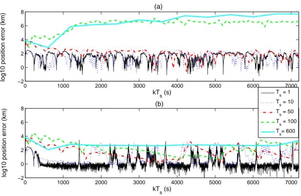
of 180deg and nondiagonal initial error covariance. . . 60 3.7 TargetxC-position-estimate errors using SDEKBF and SDUKBF. . . 61

3.8 SDEKBF and SDUKBF target position-estimate errors using time-sparse mea-surements. . . 61 3.9 SDEKBF and SDUKBF target-position estimates with an initial

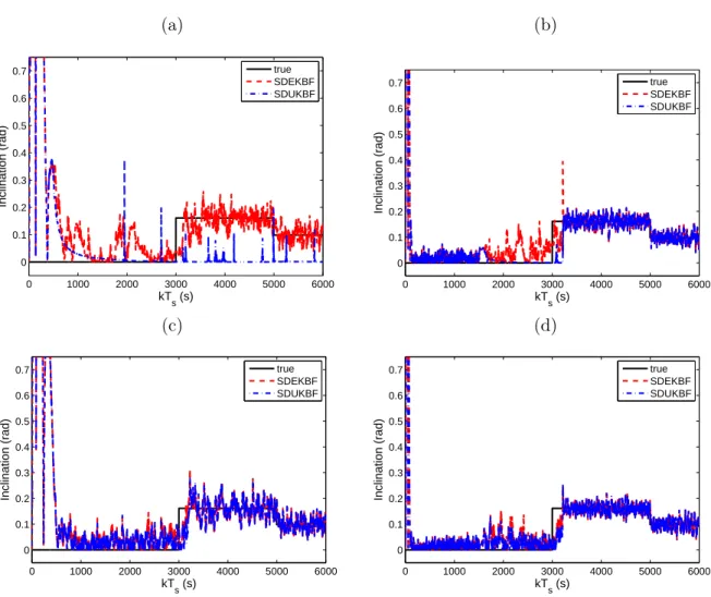
argument-of-perigee error of 180deg. . . 62 3.10 Estimated eccentricity using SDEKBF and SDUKBF. . . 63 3.11 Estimated inclination using SDEKBF and SDUKBF. . . 65 3.12 Lorenz attractor obtained by free-run simulation of its original ordinary

diﬀe-rential equations and the data-driven NARMA model. . . 71 3.13 Lorenz attractor and x2,k state component obtained by UKF with identiﬁed

(26)

3.14 The measured double scroll attractor of the implemented electronic oscillator. . 74 3.15 Attractors produced by the identiﬁed model for the electronic oscillator. . . 74 3.16 The estimated double scroll attractor of the implemented electronic oscillator. . 75 3.17 Parameter estimation for the Chua’s circuit using extended least squares and

UKF. . . 76 4.1 The projected Kalman filter by estimate projection. . . 84 4.2 The projected Kalman filter by gain projection. . . 86 4.3 The projected Kalman filter by system projection. . . 88 4.4 Diagram of the moving horizon approach . . . 94 4.5 Illustrative example of the truncation approach. . . 99 4.6 The truncated Kalman filter. . . 103 4.7 Illustrative example of the interval-constrained unscented transform compared

to the original unscented transform. . . 107 5.1 The equality-constrained Kalman ﬁlter. . . 119 5.2 Simulation of compartmental model. . . 126 5.3 Estimation of total mass for compartmental model. . . 126 5.4 Estimation errors of quaternion norm using UKF, ECUKF, PUKF-EP, and

MAUKF. . . 132 5.5 Estimation error of pendulum energy using UKF, ECUKF, PUKF-EP, and

MAUKF. . . 134 5.6 Estimate errors of angular position for the single pendulum example. . . 135 6.1 Estimate error and standard deviation for the batch reactor using unscented

ﬁlters – poor initialization case. . . 148 6.2 Estimate error and standard deviation for the continuously stirred tank reactor

using unscented ﬁlters – poor initialization case. . . 151 7.1 Diagram of the gain-constrained Kalman ﬁlter. . . 158 7.2 Data-free simulation of the van der Pol oscillator in comparison with estimated

values obtained from state-estimation algorithms for systems with unknown inputs. . . 168 7.3 Estimation errors for the Van der Pol oscillator using algorithms for systems

(27)

xxiii

7.4 Estimated input from GCUKF for the Van der Pol oscillator. . . 169 7.5 Pendulum-cart system. . . 171 7.6 Estimation errors for the pendulum-cart system using algorithms for systems

(28)

(29)

List of Symbols and Acronyms

Symbols

N _{nonnegative integers;}

Z _integers;

R _{real numbers;}

R₊ _{nonnegative real numbers;}

∈ is an element of;

△

= equals by deﬁnition;

In×n n×n identity matrix;

0n×m n×m zero matrix;

1n×m n×m unit matrix;

AT transpose ofA;

A−1 inverse ofA;

AL _{left inverse of}_A_;

AR right inverse ofA;

A1/2 _{square-root of}_A₌_A1/2₍_A1/2₎T

; A(i,j) (i,j) entry ofA;

coli(A) ith column ofA;

rowi(A) ith row of A;

det(A) determinant ofA;

diag(A) diagonal ofA;

diag(A1, . . . ,An) block-diagonal matrix;

tr(A) trace ofA;

N(A) null space ofA;

PN(A) projector with rangeN(A), wherePN(A)PN(A) =PN(A);

xi ith entry of x;

(30)

|x_| absolute value of x; ||x||2 Euclidian norm of x;

√

x square root of x;

ln(x) Neperian logarithm ofx;

log₁₀(x) logarithm with base10 of x; δ(x) Dirac-delta function atx;

max(x),min(x) maximum and minimum values ofx;

arctan(x) arc tangent of x;

sin(x),cos(x),tan(x) sine, cossine, and tangent of x;

ρ(x_|y) conditional probability density function of xgiven y;

E[_·] mathematical expectation;

¯

x mean of the random variable x;

σx standard deviation of the random variablex;

k discrete-time index;

t continuous-time index;

Ts sampling interval;

f dynamic or process nonlinear model in state space; h measurement map or observation nonlinear model; g nonlinear equality state constraint function; l nonlinear inequality state constraint function; Ak−1, Bk−1, Gk−1, Ck matrices of the linear model in state space;

Dk−1 anddk−1 matrix and vector of the linear equality state constraint;

Ek−1 and ek−1 matrix and vector of the linear inequality state constraint;

ak andbk vectors of the interval constraint on the state vector;

ˆ

Ak−1,Bˆk−1,Gˆk−1,Cˆk Jacobians of the linear model in state space; xk,x(t) state vector;

x(kTs) state vector at continuous-time sampled at timet=kTs;

uk−1,u(t) input vector;

wk−1,w(t) process noise vector;

yk,y(kTs) measurements or output vector;

vk,v(kTs) measurement noise vector;

(31)

xxvii

˘

xk,x˘(t) joint state (and parameter) vector, that is,x˘k=

h

xT_k θT_ki

T

;

˜

xk,x˜(t) augmented state vector, that is,x˜k=

h

xT_k w_kT vT_ki

T

;

˜

yk,y˜(kTs) augmented measurement vector, that is,y˜k=

h

y_kT dT_k₋₁i

T

; J(x) proﬁt or cost function ofx;

Φ(x1, . . . ,xn) functional of the sequencex1, . . . ,xn;

Wk weighting matrix;

Mk,Nk,Ok matrices of the equality constraint on the estimator gain;

ˆ

x_k_|_k₋₁ forecast state estimate;

ˆ

xk|k data-assimilation state estimate;

ˆ

θ_k_|_k data-assimilation parameter estimate;

ˆ

yk|k−1 forecast output estimate;

ˆ

xc

k|k constrained state estimate;

ˆ

xf_k_|_k,xˆb_k_|_k forward and backward state estimates;

ˆ

xs

k|k smoothed state estimate;

ˆ

xp_k_|_k projected state estimate;

ˆ

xg_k_|_k projected state estimate by gain projection;

ˆ

xt_k_|_k truncated state estimate;

ˆ ˜

x_k_|_k data-assimilation augmented state estimate;

ˆ

xi,k|k ith entry of xˆk|k;

ˆ

x_k_|_k,i data-assimilation state estimate at theith iteration at time k; ek|k−1 forecast estimation error;

e_k_|_k data-assimilation estimation error;

νk|k innovation;

P_kxx_|_k₋₁ forecast error-covariance matrix;

P_kxx_|_k data-assimilation error-covariance matrix; P_kyy_|_k₋₁ innovation covariance matrix;

P_kxy_|_k₋₁ cross-covariance matrix;

P_kxx_|_kc constrained error-covariance matrix; Pxxf

k|k,Pkxxb forward and backward error-covariance matrices; P_kxx_|_ks smoothed error-covariance matrix;

P_kxx_|_kp projected error-covariance matrix;

(32)

P_kxx_|_kt truncated error-covariance matrix; Qk−1 process-noise covariance matrix;

Rk measurement-noise covariance matrix;

˜

Rk augmented measurement-noise covariance matrix;

Kk Kalman gain at time k;

Lk constrained Kalman gain at time k;

Xj,k|k jth column of the sigma-point matrix Xk|k;

γx, γP weight vectors for calculating the state estimate and error covariance;

ΨUT unscented transform function yielding Xk|k,γx, and γP;

ΨICUT interval-constrained unscented transform function yielding Xk_|k and γk.

Acronyms

CDF Central Diﬀerence Filter;

CEKF Constrained Extended Kalman Filter;

CKF Constrained Kalman Filter;

CIUKF Constrained Interval Unscented Kalman Filter;

CPU Central Processing Unit;

CUKF Constrained Unscented Kalman Filter;

DDF Divided Diﬀerence Filter;

ECKF Equality-Constrained Kalman Filter;

ECUKF Equality-Constrained Unscented Kalman Filter;

EKF Extended Kalman Filter;

EKS Extended Kalman Smoother;

EnKF Ensemble Kalman Filter;

ERR Error Reduction Error;

FPR Flight Path Reconstruction;

GCKF Gain-Constrained Kalman Filter;

GCKP Gain-Constrained Kalman Predictor;

GCUKF Gain-Constrained Unscented Kalman Filter;

GPS Global Positioning System;

(33)

xxix

ICUT Inequality-Constrained Unscented Transfom;

IEKF Iterated Extended Kalman Filter;

IMU Inertial Measurement Unit;

IUKF Interval Unscented Kalman Filter;

KF Kalman Filter;

KP Kalman Predictor;

KS Kalman Smoother;

LECUKF Equality-Constrained Unscented Kalman Filter;

LEO Low-Earth Orbit;

LUKF Localized Unscented Kalman Filter;

MAEKF Measurement-Augmentation Extended Kalman Filter; MAKF Measurement-Augmentation Kalman Filter;

MAEKF Measurement-Augmentation Unscented Kalman Filter; MEMS Micro-Electro-Mechanical Systems;

MHD Magnetohydrodynamics;

MHE Moving Horizon Estimator;

MT Mean Trace;

NARMA Nonlinear Autoregressive Moving Average;

NED North-East-Down;

NMHE Nonlinear Moving Horizon Estimator;

ODE Ordinary Diﬀerential Equation;

PDF Probability Density Function;

PEKF-EP Projected Extended Kalman Filter by Estimate Projection;

PF Particle Filter;

PKF-EP Projected Kalman Filter by Estimate Projection; PKF-GP Projected Kalman Filter by Gain Projection;

PKF-IC Projected Kalman Filter for Inequality-Constrained Systems; PKF-SP Projected Kalman Filter by System Projection;

PLUKF Localized Unscented Kalman Filter; PUKF Projected Unscented Kalman Filter;

PUKF-EP Projected Unscented Kalman Filter by Estimate Projection;

RMSE Root Mean Square Error;

(34)

RTS Rauch-Tung-Striebel;

SCKF Spatially Constrained Kalman Filter;

SDEKBF Sampled-Data Extended Kalman-Bucy Filter; SDREF State-Dependent Ricatti Equation Filter; SDUKBF Sampled-Data Unscented Kalman-Bucy Filter; SIUKF Sigma-Point Interval Unscented Kalman Filter;

SPKF Sigma-Point Kalman Filters;

TKF Truncated Kalman Filter;

TIUKF Truncated Interval Unscented Kalman Filter; TPUKF Two-Step Projected Unscented Kalman Filter; TUKF Truncated Unscented Kalman Filter;

UKF Unscented Kalman Filter;

UKS Unscented Kalman Smoother;

UnbKF-UI Unbiased Kalman Filter with Unknown Inputs;

URNDDR Unscented Recursive Nonlinear Dynamics Data Reconciliation;

(35)

Resumo Estendido

Apresenta-se a seguir um resumo estendido relativo ao projeto de pesquisa desen-volvido nesta tese. Primeiramente, introduz-se o problema estudado, motivando-o por meio de uma breve revisão bibliográﬁca e explicitando os objetivos da presente tese. Em seguida, discutem-se brevemente as contribuições desenvolvidas neste projeto, quer as de cunho prático, quer as de conteúdo teórico. Finalmente, as conclusões são apresentadas.

Introdução

Motivação

Estudos astronômicos, em especial no fim do século XVIII, serviram como um dos principais e pioneiros estímulos ao desenvolvimento da teoria de estimação. Visando a estimar os parâmetros das equações de movimento de planetas e cometas a partir de dados medidos por telescópios, Gauss propôs o método dos mínimos quadrados em 1795 (Sorenson, 1970). Pouco mais de um século e meio depois, incentivado pelo início da corrida espacial, em janeiro de 1959, Rudolf Kalman, por meio de “um único, gigante e persistente exercício matemático” (Kalman, 2003) inventou o algoritmo de filtragem (Kalman, 1960), o qual leva seu nome, em reconhecimento ao considerado, por muitos, até hoje, o principal trabalho científico sobre estimação de estados. Atualmente, o filtro de Kalman é solução de prateleira para muitos problemas do setor aeroespacial (Cipra, 1993; de Moraes et al., 2007). Além disso, sua aplicação estende-se do treinamento de redes neurais (Rios Neto, 1997) à predição metereológica (Carme et al., 2001).

Apesar do amplo uso do ﬁltro de Kalman (KF), as premissas de linearidade e Gaus-sianidade que lhe garantem otimalidade impedem sua aplicação em sistemas não-lineares. Métodos de ﬁltragem de partículas (PF) podem ser empregados para, de forma aproximada, tratar sistemas não-lineares e não-gaussianos (Gordon et al., 1993; Arulampalam et al., 2002).

(36)

No entanto, seu elevado custo computacional inviabiliza sua implementação em várias apli-cações de tempo real (Daum, 2005).

Por outro lado, métodos de aproximação gaussiana contornam tal dificuldade pelo emprego de algoritmos baseados no KF. Desse grupo, o filtro de Kalman estendido (EKF) (Schmidt, 1970; Jazwinski, 1970), cujo cerne está na linearização analítica ou numérica do modelo do sistema, é a solução mais usada nas últimas quatro décadas. No entanto, EKF apresenta algumas limitações como sensibilidade às condições iniciais e à sintonia das ma-trizes de covariância de ruído, especialmente, para sistemas fortemente não-lineares. Nesse caso, pode-se observar divergência ou mesmo instabilidade do estimador (Reif et al., 1999). Alternativamente, o filtro de Kalmanunscented(UKF) (Julier et al., 1995; Julier & Uhlmann, 2004), um algoritmo da família dos filtros de Kalman de pontos sigma (SPKF) (Lefebvre et al., 2002; van der Merwe et al., 2004), usa uma técnica de linearização estatística que emprega um número reduzido de amostras escolhidas deterministicamente (Julier et al., 2000). Vários trabalhos recentes (Julier et al., 2000; Haykin, 2001; van der Merwe et al., 2004; Lefebvre et al., 2004; Romanenko & Castro, 2004; Hovland et al., 2005; Choi et al., 2005; Crassidis, 2006) relatam o desempenho superior do UKF comparado ao EKF. Portanto, nesta tese, são desenvolvidos algoritmos baseados no UKF.

KF é o estimador de estados ótimo para sistemas lineares e Gaussianos que usa duas fontes de informação incertas, a saber: um modelo matemático (usado na etapa de predição) e as medições (usadas na etapa de assimilação de dados). Em alguns casos, contudo, informação adicional sobre o sistema pode ser conhecida, e essa terceira fonte de informação pode ser útil para melhorar as estimativas de estado. Nesta tese, é considerado o cenário no qual a dinâmica e os distúrbios do sistema são tais que o vetor de estados satisfaz uma restrição de desigualdade (Rao, 2000; Robertson & Lee, 2002; Goodwin et al., 2005) ou uma restrição de igualdade (Teixeira et al., 2007; Ko & Bitmead, 2007). Por exemplo, em reações químicas, as concentrações dos reagentes e produtos são não-negativas (Massicotte et al., 1995; Chaves & Sontag, 2002), ao passo que no problema de estimação de atitude com parametrização em quatérnios, o vetor de atitude deve ter norma unitária (Crassidis & Markley, 2003).

(37)

xxxiii

Formulação do Problema

Para o sistema dinâmico estocástico não-linear de tempo discreto

xk = f(xk−1, uk−1, wk−1, k−1), (1)

yk = h(xk, vk, k), (2)

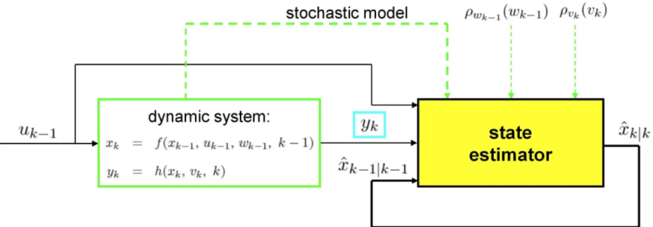
em quef :Rn×Rp×Rq×N→Rne_h_:Rn×Rr×N→Rmsão, respectivamente, os modelos de processo e de observação, os quais são assumidamente conhecidos, o problema de estimação de estados é deﬁnido a seguir; veja a Figura 1.1. Assuma que, para todok≥1, são conhecidas as medições yk∈Rm, as entradas uk−1 ∈Rp, e as funções de densidade de probabilidade (PDF)

ρx0(x0), ρwk−1(wk−1) e ρvk(vk), em que x0 ∈ R

n _{é o vetor de estados inicial,} _w

k−1 ∈ Rq é o

ruído de processo, representando pertubações desconhecidas, e vk∈Rr é o ruído de medição, o qual trata das incertezas nas observações. Deﬁna a função de lucro

J(xk)△=ρ(xk|(y1, . . . ,yk)), (3)

em queρ(xk|(y1, . . . ,yk))é a PDF condicional a posteriorido vetor de estadosxk∈Rn condi-cionada às medições passadas y1, . . . , yk−1 e presente yk. A solução completa do problema de estimação de estados é dada por ρ(xk|(y1, . . . ,yk)) e o maximizador xˆk|k ∈ Rn de J é a

estimativa de estadosótima.

Conforme mencionado anteriormente, para sistemas lineares e Gaussianos, KF fornece a solução recursiva ótima para o problema de estimação de estados. Para o caso não-linear, todavia, a solução para esse problema é complicada devido ao fato de ρ(xk|(y1, . . . ,yk)) não ser completamente caracterizada por sua média e covariância (Daum, 2005). Dessa maneira, aproximações baseadas no KF são investigadas nesta tese.

Neste trabalho, considera-se que o vetor de estados está sujeito à restrição de igualdade

g(xk, k−1) = dk−1, (4)

e/ou à restrição de desigualdade

l(xk, k−1) ≤ ek−1, (5)

(38)

maximizadorxˆc

k|k de (3) sujeito a (4) e/ou (5) é a estimativa de estado restritaótima. Neste trabalho, também se estuda a restrição de intervalo

ak ≤ xk ≤ bk, (6)

em queai,k < bi,k,i= 1, . . . ,n, a qual é um caso especial de (5).

Objetivos

Esta tese trata do desenvolvimento de algoritmos de estimação de estados para sis-temas lineares e não-lineares com o uso de conhecimento a priori na forma de restrições. Ademais, investigam-se aplicações de engenharia para esses algoritmos. Dessa maneira, cinco são os objetivos deste projeto de pesquisa, a saber:

1. Estudar e deduzir uma solução ótima para o problema de estimação de estados com res-trição de igualdade no vetor de estados para sistemas lineares, bem como soluções apro-ximadas para sistemas não-lineares. Para o último caso, usa-se a abordagemunscented. Investigar os problemas de estimação de atitude com parametrização em quatérnios (Crassidis & Markley, 2003) e assimilação de dados em magneto-hidrodinâmica com divergência nula (Tóth, 2000).

2. Propor e comparar algoritmos sub-ótimos de estimação de estados baseados no UKF para impor restrições de intervalo nas estimativas de estado de sistemas não-lineares. 3. Desenvolver uma metodologia geral em estimação de estados com restrição de igualdade

no ganho do estimador a ﬁm de impor propriedades especiais nas estimativas de estado. Mostrar como outros algoritmos propostos na literatura (Kitanidis, 1987; Darouach et al., 2003; Palanthandalam-Madapusi et al., 2006; Gillijns & De Moor, 2007b; Chandrasekar et al., 2007; Gupta & Hauser, 2007) são casos especiais dessa metodologia, bem como estender o algoritmo obtido para o caso não-linear usando a abordagemunscented. 4. Ilustrar a aplicação de ﬁltros de Kalman não-lineares para solução de dois problemas

em engenharia aeroespacial: reconstrução de trajetórias de vôo (Mulder et al., 1999; Fagundes, 2007; Mendonça et al., 2007) e estimação de trajetórias de espaçonaves (Tapley et al., 2004; de Moraes et al., 2007).

(39)

xxxv

caótica (Fiedler-Ferrara & Prado, 1994) usando modelos identiﬁcados de tempo discreto (Aguirre, 2007) e UKF. Além disso, deseja-se discutir o impacto do não conhecimento das equações dinâmicas exatas e do uso de modelos aproximados.

Estudos de Caso de Estimação de Estados Sem Restrições

Reconstrução de Trajetórias de Vôo

O problema de reconstrução de trajetórias de vôo (FPR) (Mulder et al., 1999; de Mendonça, 2005) é o primeiro passo no procedimento de se usar dados de ensaios de vôo para obter informação sobre os parâmetros do modelo de uma aeronave (Hemerly et al., 2003; Góes et al., 2006; Jategaonkar, 2006). Basicamente, essa reconstrução signiﬁca estimar a trajetória da aeronave a partir de dados de instrumentação nela instalada. Esse passo é crucial e fundamental, pois sensores reais apresentam polarização, a qual deve ser considerada nos estágios subsequentes de análise dos dados. Valores estimados para polarização podem ser obtidos pelo processo de FPR.

Nesta tese, o problema de reconstrução de trajetórias de vôo é abordado no contexto de métodos de filtragem de Kalman não-linear. Procura-se elucidar três questões quanto: (i) à escolha do algoritmo de filtragem de Kalman não-linear empregado – EKF ou UKF; (ii) ao uso de um algoritmo de suavização no lugar de um método de filtragem; e (iii) ao emprego de uma abordagem iterativa de filtragem para melhorar as estimativas.

(40)

em termos de precisão.

Estimação de Trajetórias de Espaçonaves

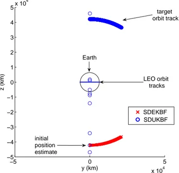
O presente estudo de caso ilustra e compara ﬁltros de Kalman não-lineares para o pro-blema de estimação de trajetórias de espaçonaves (Tapley et al., 2004; Curtis, 2005). Diferentes problemas e formulações podem ser considerados para estimação de trajetória de espaçonaves com base no número e tipo de medições disponíveis, incluindo distância (Duong & Winn, 1973; Pisacane et al., 1974), variação de distância (Bizup & Brown, 2004) e ângulo (Fowler & Lee, 1985; Lee & Alfriend, 2007). O caso em que as medições são fornecidas por uma constelação de satélites é estudado em (Cicci & Ballard, 1994a,b; Chiaradia et al., 2003; de Moraes et al., 2007).

São utilizados algoritmos de ﬁltragem de tempo contínuo com medições amostradas (de seis satélites com órbita equatorial de baixa altitude) baseados no EKF (Jazwinski, 1970; Gelb, 1974) e UKF (Särkkä, 2007) para rastrear a órbita de um satélite em órbita geossíncrona de elevada altitude.

Utilizam-se dados simulados na presente análise. Os resultados obtidos são exibidos nas Figuras 3.6, 3.7, 3.8, 3.9, 3.10 e 3.11 e Tabelas 3.3 e 3.4. A abordagemunscentedmostrou-se menos sensível à inicialização e ao intervalo de amostragem das medições do que a abordagem estendida. No entanto, o método baseado no UKF apresenta um custo computacional cerca de duas vezes maior. Além disso, o algoritmo unscented produz estimativas mais precisas para a excentricidade da órbita, quando comparado ao algoritmo estendido. Finalmente, a ﬁm de estimar a inclinação da órbita da espaçonave, o uso de medições de ângulo ajudam na convergência e melhoram o desempenho de ambos os algoritmos.

Uso de Modelos Identificados em Filtragem Unscented

(41)

xxxvii

de estados estão disponíveis durante um curto intervalo de tempo para construir o modelo, enquanto somente uma componente do vetor de estados é medida para uso no algoritmo de ﬁltragem. Para tal, utilizam-se dados simulados do sistema de Lorenz (Lorenz, 1963) e dados experimentais de um oscilador eletrônico conhecido como circuito de Chua (Chua, 1994; Tôrres & Aguirre, 2000).

A partir dos testes realizados, cujos resultados são mostrados nas Figuras 3.12, 3.13, 3.15, 3.16 e 3.17 e Tabelas 3.5 e 3.6, relata-se que UKF é viável para estimar conjuntamente estados e parâmetros desses sistemas não-lineares caóticos a partir de modelos previamente identificados. Nesse cenário, a definição apropriada da matriz de covariância de ruído de processo parece ser fundamental na convergência do algoritmo de filtragem. Modelos ruins, geralmente, resultam em estimativas de estado pouco precisas ou em divergência do estimator, independente do valor atribuído a tal matriz, ao passo que o emprego de modelos mais precisos melhoram o desempenho das estimativas de estado, especialmente, para altos níveis de ruído nas medições.

Contribuições Teóricas em Estimação de Estados Com Restrições

Estimação de Estados com Restrições de Igualdade

Diversos métodos têm sido desenvolvidos para estimação de estados com restrições de igualdade. Uma das técnicas mais populares é o ﬁltro de Kalman com medições aumentadas (MAKF), para o qual “medições” perfeitas das grandezas de restrição são anexadas às medições físicas (Porrill, 1988; Tahk & Speyer, 1990; Wen & Durrant-Whyte, 1992). Além disso, são apresentados os métodos de projeção das estimativas (Simon & Chia, 2002), projeção do sistema (Ko & Bitmead, 2007) e projeção do ganho (Gupta & Hauser, 2007).

As abordagens de medições aumentadas e projeção das estimativas são estendidas para o caso não-linear por meio do EKF (Alouani & Blair, 1993; Chen & Chiang, 1993; Simon & Chia, 2002; Gupta, 2007b). Alternativamente, um algoritmo de projeção de duas etapas para tratar restrições de igualdade não-lineares é apresentado em (Julier & LaViola Jr., 2007). Além disso, um método que usa multiplicadores de Lagrange é capaz de impor exatamente restrições de igualdade quadráticas e unidimensionais (Yang & Blasch, 2006). A Tabela 4.1 compara os principais métodos apresentados na literatura para impor restrições de igualdade lineares e não-lineares nas estimativas de estado.

(42)

igual-dade, primeiramente considera-se o caso linear e Gaussiano. Nesse contexto, mostra-se como a existência de restrições de igualdade está vinculada à deﬁnição de ruído de processo e equações dinâmicas com propriedades especiais, as quais são resumidas nas equações (5.5)-(5.7). Assim, o ﬁltro de Kalman com restrições de igualdade (ECKF) é derivado como a solução recursiva ótima (sob a ótica de máximoa posteriori) para o problema em questão; veja o Teorema 5.2.1. ECKF é comparado a quatro algoritmos alternativos apresentados na literatura. O algoritmo proposto e os quatro revisados são ilustrados por meio de dois exemplos: sistema de compar-timentos para o qual oberva-se conservação de massa (veja a Figura 5.3 e a Tabela 5.1) e um sistema de rastreamento de veículo terrestre com restrições cinemáticas (veja a Tabela 5.2).

Para o caso não-linear, três algoritmos sub-ótimos baseados no UKF são apresentados, a saber: ﬁltro de Kalmanunscented com restrições de igualdade (ECUKF), ﬁltro de Kalman

unscented projetado por projeção das estimativas (PUKF-EP), e ﬁltro de Kalman unscented

com medições aumentadas (MAUKF). Dois exemplos são considerados: estimação de atitude com parametrização em quatérnios (veja a Figura 5.4 e a Tabela 5.3) e um pêndulo simples com conservação de energia mecânica, para o qual um modelo discretizado sem conservação de energia é usado (veja as Figuras 5.5 e 5.6 e as Tabelas 5.4 e 5.5).

A partir dos resultados obtidos para as quatro aplicações investigadas, observou-se que, além de impor uma restrição de igualdade conhecidaa priori, os métodos propostos pro-duzem estimativas de estado mais precisas e informativas que KF (para o caso linear) ou UKF (no caso não-linear). Além disso, todas as abordagens investigadas têm custo computacional semelhante e competitivo ao do KF (para algoritmos lineares) e UKF (caso não-linear).

Quanto à escolha do algoritmo, ECKF e os quatro métodos revisados produzem resul-tados de desempenho semelhante para o caso linear. No entanto, para o caso não-linear, com base nos exemplos investigados, recomenda-se testar, na seguinte ordem, ECUKF, MAUKF e PUKF-EP para uma dada aplicação. Observe que, como tais métodos são aproximados, o desempenho dos mesmos depende da aplicação.

Estimação de Estados com Restrições de Intervalo

(43)

xxxix

do KF e apropriada sintonia de suas matrizes de covariância de ruído. O procedimento de truncamento (Shimada et al., 1998; Simon & Simon, 2007) remodela a PDF computada pelo KF, a qual é assumidamente Gaussiana e é dada pela estimativa de estados e pela covariân-cia do erro de estimação, nas bordas da restrição de desigualdade. Finalmente, por meio da abordagem de projeção (Simon & Simon, 2006b), se a estimativa de estados não satisfaz a restrição de desigualdade, então a mesma é projetada no extremo da região de restrição.

Para sistemas não-lineares, algoritmos baseados no MHE têm sido empregados (Rao et al., 2003; Russo & Young, 1999). No entanto, como essas técnicas são não-recursivas, elas são computacionalmente inviáveis para algumas aplicações em tempo real (Vachhani et al., 2006). Para esses casos, o ﬁltro de Kalman estendido restrito (CEKF) (Vachhani et al., 2006; Marcon et al., 2002), o qual é um caso especial do MHE com horizonte móvel unitário e é chamado de algoritmo recursivo de reconciliação de dados para sistemas dinâmicos não-lineares (RNDDR) em (Vachhani et al., 2005), é apresentado como um algoritmo de implementação mais simples e de menor custo computacional. Motivado pelo desempenho superior do UKF com relação ao EKF, o algoritmo unscented recursivo de reconciliação de dados para sistemas dinâmicos não-lineares (URNDDR), o qual, por conveniência, é chamado de ﬁltro de Kalman unscented

intervalar de pontos sigma (SIUKF) nesta tese, é apresentado em (Vachhani et al., 2006). Os algoritmos supracitados são comparados na Tabela 4.1.

Nesta tese, é estudado o problema de estimação de estados com restrições de intervalo para sistemas não-lineares. Pela combinação de uma de duas possíveis abordagens unscented

para execução da etapa de predição e um de cinco possíveis candidatos para a etapa de assi-milação de dados – as quais são usadas na literatura e listadas na Tabela 6.1, são propostos os seguintes algoritmos: ﬁltro de Kalmanunscentedrestrito (CUKF), ﬁltro de Kalmanunscented

restrito intervalar (CIUKF), ﬁltro de Kalman unscented intervalar (IUKF), ﬁltro de Kalman

unscented truncado (TUKF), ﬁltro de Kalman unscented truncado intervalar (TIUKF), ﬁltro de Kalmanunscented projetado (PUKF).

(44)

que CIUKF e IUKF têm desempenho intermediário. Com relação ao custo computacional, IUKF, TIUKF, e TUKF são competitivos com UKF. Ademais, CUKF, CIUKF e PUKF são mais lentos que UKF, já que requerem a soluçãoonline de problemas de otimização. Por essa razão, SIUKF é o algoritmo mais lento.

Todavia, não é possível indicar qual método é mais adequado para um dado problema. Na verdade, parece que a escolha do método depende da aplicação. A partir dos dois exem-plos investigados, considerando o compromisso entre precisão e complexidade computacional, TUKF e TIUKF parecem ser as melhores alternativas, seguidos por SIUKF, CIUKF, e IUKF.

Estimação de Estados com Restrição no Ganho

Em estimação de estados clássica, o ganho padrão do estimador é irrestrito no sentido de que todos os resíduos das medições são potencialmente usados para diretamente corrigir todas as componentes do vetor de estados. Semelhante ao caso de controle realimentado com saída estática (Syrmos et al., 1997), o qual pode ser visto como uma forma restrita do controle realimentado com vetor de estados completo, é possível restringir a forma do ganho do estimador. Fazendo isso, é possível impor propriedades especiais nas estimativas de estado. Três distintas motivações para restringir o ganho do estimador são encontradas na literatura. Primeiramente, em (Kitanidis, 1987; Darouach et al., 2003; Palanthandalam-Madapusi et al., 2006; Gillijns & De Moor, 2007a,b; Gillijns, 2007), o ganho do estimador é restrito a fim de se obter estimativas não polarizadas apesar do fato de entradas exógenas desconhecidas (podendo ser determinísticas ou de média não-nula) serem presentes. Trata-se do filtro de Kalman não-polarizado com entradas desconhecidas (UnbKF-UI). De forma seme-lhante, em (Chandrasekar & Bernstein, 2006; Chandrasekar et al., 2007), o ganho é restrito para simplificar a estrutura do estimador e sua implementação com multi-processadores para aplicações envolvendo sistemas de dimensão elevada, tais como aqueles que envolvem equações diferenciais parciais discretizadas. A mesma idéia pode ser aplicada para tratar falha sensorial parcial ou completa. O algoritmo resultante é chamado de filtro de Kalman espacialmente restrito (SCKF). Finalmente, em (Gupta & Hauser, 2007), é apresentado o filtro de Kalman projetado com ganho projetado (PKF-GP), cujo ganho é restrito para produzir estimativas de estado satisfazendo uma restrição de igualdade linear. Portanto, desenvolve-se uma metodolo-gia geral que inclui os métodos supracitados como casos especiais e que permite a futura proposição de novos estimadores de estados com ganho restrito.

(45)

xli

ótima de variância mínima para o problema de estimação de estados com restrição no ganho para sistemas lineares; veja a Proposição 7.1.2. Ademais, KF, UnbKF-UI, SCKF e PKF-GP são apresentados como casos especiais do GCKF. Também é derivado o preditor de Kalman com ganho restrito para o mesmo problema.

Além disso, usando a transformadaunscented, o ﬁltro de Kalmanunscentedcom ganho restrito (GCUKF) é apresentado como extensão não-linear do GCKF. Embora esse algoritmo seja uma solução aproximada para o problema de estimação de estados não-linear, seu ganho satisfaz exatamente a restrição de igualdade.

Dois exemplos de sistemas não-lineares, a saber, o oscilador de van der Pol e um sistema pêndulo-carro, são usados para ilustrar uma aplicação do GCUKF na qual o vetor de entrada é desconhecido e deseja-se obter estimativas de estado não-polarizadas. Os resultados obtidos são mostrados nas Figuras 7.2, 7.3, 7.4 e 7.6 e Tabelas 7.1 e 7.2. Em ambos os casos, por meio do GCUKF, obtiveram-se estimativas de estados melhores do que aquelas obtidas pelo UKF com o vetor de entradas desconhecido.

Conclusões

Na presente tese, além de apresentar uma revisão do atual estado da arte em esti-mação de estados com restrições, são desenvolvidos métodos de ﬁltragem de Kalman para impor restrições de igualdade e/ou de desigualdade na estimativa de estado. Ambos os casos de sistemas lineares e não-lineares são considerados. Para o último caso, propõem-se algo-ritmos baseados no ﬁltro de Kalman unscented. Ademais, propõe-se uma metodologia geral para estimação de estados com uma restrição de igualdade no ganho do estimador, visando a impor indiretamente propriedades especiais na estimativa de estado. Exemplos simulados e experimentais são usados para ilustrar os algoritmos estudados e propostos ao longo desta tese.

(46)

(47)

Chapter 1

Introduction

“If I have seen further, it is by standing on the shoulders of giants.”

Isaac Newton

1.1 Motivation

Astronomical studies provided the pioneer stimuli for the development of the estima-tion theory especially in the end of the 18th century. According to (Sorenson, 1970), Karl Friedrich Gauss was the leading protagonist of the birth of this theory, when he investigated the motion of planets and comets using data measured from telescopes. Aiming at estima-ting the parameters that characterize the equations of motion of these heavenly bodies, Gauss derived the well-known least-squares method in 1795.

About a century and a half later, the advent of the space race provided the main motivations for the development of the state-estimation theory.1

Aerospace scientists were looking for a solution to the spacecraft trajectory estimation problem, for instance. Then, in the January of 1959, Rudolf Emil Kalman, by means of a “single, gigantic, persistent mathe-matical exercise” (Kalman, 2003) proposed the state-estimation algorithm (Kalman, 1960) that is named after him in recognition to the major breakthrough ever made in the field of state estimation. One of the first and most important applications of the Kalman filtering theory was in the on-board computer that guided the descent of the Apollo 11 lunar module to the moon (Schmidt, 1981). Currently, Kalman-like algorithms are the off-the-shelf technology to many applications in industry, including navigation systems (Cipra, 1993). At this point, it is important to recognize the previous outstanding theoretical contributions to the development of the state-estimation theory given by Fisher (1912), Wiener (1949), and Kolmogorov (1962), among others.

1

(48)

Similar to Gauss, Kalman also formulated his problem as an optimization problem that minimizes a functional of the square of the estimation error, but, unlike Wiener (1949), he used the state-space formulation. Kalman’s achievements in state estimation agree with the Albert Einstein’s quote that says that “the mere formulation of a problem is far more often essential than its solution, which may be merely a matter of mathematical or experimental

skill.”

Nevertheless, the Gauss’ legacy was not the main source of inspiration for Kalman’s work. Kalman (2003) argues that his work was naturally inspired by the technological revo-lution created by Isaac Newton. In 1687, using only mathematical reasoning, Newton proved that the gravitational force causes the motion of the planets around the Sun, confirming thus the Kepler’s laws. According to Kalman, the revolutionary ideas inherited from Newton were the use of data to the detriment of physical assumptions to formulate a problem and the mathematization of the problem to build a solution. This approach is still responsible for many technological innovations nowadays. We mention, for instance, the increasing effort to-wards the use of data collected from onboard instrumentation during flight tests to determine the parameters of aircraft models (Jategaonkar, 2006; Góes, Hemerly, Maciel, Rios Neto, de Mendonça & Hoff, 2006).

1.1.1 Unconstrained State Estimation

The assumption of linear dynamics and linear meaurement map, as well as the as-sumption of Gaussian distribution of the disturbances, restrict the use of the classical Kalman ﬁlter (KF) in some practical cases. Therefore, methods for the nonlinear scenario are necessary. The extended Kalman ﬁlter (EKF) is the straightforward extension of KF to the nonlinear case by means of analytical or numerical linearization of the system equations (Schmidt, 1970; Jazwinski, 1970). EKF has been the most widely used algorithm for nonlinear state estima-tion during the last four decades, covering applicaestima-tions from spacecraft trajectory estimaestima-tion (Schmidt, 1981; de Moraes, da Silva & Kuga, 2007) and weather forecasting (Carme, Pham, & Verron, 2001) to training of neural networks (Rios Neto, 1997).

(49)

1.1 Motivation 3

(Julier, Uhlmann & Durrant-Whyte, 1995; Julier & Uhlmann, 2004). UKF is based on “the intuition that it is easier to approximate a probability distribution than it is to approximate an

arbitrary nonlinear function or transformation” (Julier, Uhlmann & Durrant-Whyte, 2000). Like UKF, other nonlinear methods (Ito & Xiong, 2000; Nogaard, Poulsen & Ravn, 2000) use the same principles and are categorized into the sigma-point Kalman ﬁlter (SPKF) framework (Lefebvre, Bruyninckx & De Schutter, 2002; van der Merwe, 2004).

Alternatively, since the decade of 1990, particle ﬁltering methods have been proposed (Gordon, Salmon & Smith, 1993); see (Arulampalam, Maskell, Gordon & Clapp, 2002) for a helpful overview. Such methods are able to treat non-Gaussian distributions, as well as nonli-nearity in the dynamics and measurement map. However, the high computational complexity of these methods inhibits their real-time application in some practical cases (Daum, 2005).

Along the last eight years, an impressive number of applications of SPKF algorithms has been reported, such as,

• in sensor fusion and navigation (Hall & Llinas, 2001; Wagner & Wieneke, 2003; Azizi & Houshargi, 2003; Shin & El-Sheimy, 2003; van der Merwe, Wan & Julier, 2004; Crassidis, 2006; Metzger, Wisotzky, Wendel & Trommer, 2005);

• target tracking (Farina, Ristic & Benvenuti, 2002; Ristic, Farina, Benvenuti & Arulam-palam, 2003);

• spacecraft attitude estimation (Chen, Seereeram & Mehra, 2003; Crassidis & Markley, 2003; Markley, Crassidis & Cheng, 2005; Psiaki, 2005; VanDyke, Schwartz & Hall, 2004; Teixeira, Chandrasekar, Tôrres, Aguirre & Bernstein, 2008b) and spacecraft trajectory estimation (Lee & Alfriend, 2007; Teixeira, Santillo, Erwin & Bernstein, 2008);

• ﬂight path reconstruction (Teixeira, Tôrres, Iscold & Aguirre, 2005; de Mendonça & Hemerly, 2007);

• aircraft failure detection (Brunke & Campbell, 2002, 2004);

• state-and-parameter estimation in nonlinear dynamics and chaos (Sitz, Schwarz, Kurths & Voss, 2002; Sitz, Schwarz & Kurths, 2004; Aguirre, Teixeira & Tôrres, 2005);

• parameter estimation of continuous-time diﬀerential equations (Voss, Timmer & Kurths, 2004) and multilayer perceptron neural networks (Haykin, 2001; Wan, van der Merwe & Nelson, 2000; Feldkamp, Feldkamp & Prokhorov, 2001; Choi, Yeap, & Bouchard, 2004; Choi, Yeap & Bouchard, 2005);

(50)

• data assimilation for large-scale systems (Chandrasekar, 2007; Chandrasekar, Ridley & Bernstein, 2007);

• state estimation for chemical processes (Hovland, von Hoﬀ, Gallestey, Antoine, Farruggio & Paice, 2005; Vachhani, Narasimhan & Rengaswamy, 2006; Teixeira, Tôrres, Aguirre & Bernstein, 2008), induction motors (Akin, Orguner & Ersak, 2003), and solar power plants (Hovland, von Hoﬀ, Gallestey, Antoine, Farruggio & Paice, 2005).

Therefore, we believe that the sigma-point approach is the current state of the art in nonli-near state estimation. In this thesis, we focus on sigma-point algorithms for nonlinonli-near state estimation.

1.1.2 Equality and Inequality State-Constrained State Estimation

The classical KF for linear systems provides optimal state estimates under standard noise and model assumptions. In practice, however, additional information about the system may be available, and this information may be useful for improving state estimates. A scenario we have in mind is the case in which the dynamics and the disturbances are such that the states of the system satisfy an equality (Teixeira, Chandrasekar, Tôrres, Aguirre & Bernstein, 2007; Ko & Bitmead, 2007) or inequality constraint (Rao, 2000; Robertson & Lee, 2002; Goodwin, Seron & de Doná, 2005).

(51)

1.1 Motivation 5

Sukkarieh & Nebot, 2001; Alouani & Blair, 1993; Shen, Honga & Cong, 2006). In such cases, we wish to obtain state estimates that take advantage of prior knowledge of the states and use this information to obtain better estimates than those provided by KF in the absence of such information. Although it is diﬃcult to make correspondingly precise statements in the case of nonlinear systems, the same principles and objectives apply.

Constrained state estimation has been receiving increasing attention in both academia and industry, especially in the last ten years (Simon, 2008). Various methods have been de-veloped for equality-constrained state estimation. One of the most popular techniques is the measurement-augmentation Kalman ﬁlter, in which a perfect “measurement” of the cons-trained quantity is appended to the physical measurements (Porrill, 1988; Tahk & Speyer, 1990; Chia, Chow & Chizeck, 1991; Wen & Durrant-Whyte, 1992; Doran, 1992). In addi-tion, estimate-projection (Simon & Chia, 2002), system-projection (Ko & Bitmead, 2007), and gain-projection (Gupta & Hauser, 2007) methods have been considered. Alternatively, the model reduction approach, in which the model parameterization is reduced by substitut-ing the equality constraint into the dynamic model, can be employed (Wen & Durrant-Whyte, 1991; Simon, 2006).

The measurement-augmentation and estimate-projection approaches are also extended to the nonlinear case by means of EKF, yielding the approximate nonlinear equality-constrained algorithms: measurement-augmentation EKF (Alouani & Blair, 1993; Chen & Chiang, 1993; Walker, 2006) and projected EKF (Simon & Chia, 2002; Gupta, 2007b), respectively. A two-step projection algorithm for handling nonlinear equality constraints has also been presented (Julier & LaViola Jr., 2007). Also, a Lagrange-multiplier method for exactly enforcing a single quadratic nonlinear state constraint is given in (Yang & Blasch, 2006).

(52)

2006; Simon & Simon, 2006b).

For nonlinear inequality-constrained systems, algorithms based on MHE are employed (Rao, Rawlings & Mayne, 2003; Haseltine & Rawlings, 2005; Russo & Young, 1999). However, since these techniques are non-recursive, they are computationally expensive and diﬃcult to use in real-time applications (Vachhani et al., 2006). For such cases, the constrained EKF (Rao, Rawlings & Mayne, 2003; Vachhani, Narasimhan & Rengaswamy, 2006; Marcon, Trieiweiler & Secchi, 2002), which is a special case of MHE with unitary moving horizon and is called recursive nonlinear dynamics data reconciliation (RNDDR) in (Vachhani et al., 2005, 2006), is presented as a simpler and less computationally demanding algorithm. Motivated by the improved performance (Julier et al., 2000; Lefebvre et al., 2002, 2004; van der Merwe et al., 2004; Reif et al., 1999) of UKF over EKF, the unscented RNDDR, which is referred to as the sigma-point interval unscented Kalman ﬁlter in this thesis, is presented in (Vachhani et al., 2006).

1.1.3 Gain-Constrained State Estimation

State estimation is eﬀectively a closed-loop problem, in which data are fed back to the plant. Like servo control, the state estimator acts based on an error signal, namely, the innovation, and uses statistical information to determine a “feedback” gain that can produce optimal or suboptimal state estimates. This data-injection process is analogous to full-state feedback control.

In classical state estimation, the standard data injection gain is unconstrained in the sense that all measurement residuals are potentially used to directly update all of the state estimates. Just as static output feedback control (Syrmos, Abdallah, Dorato & Grigoriadis, 1997) can be viewed as a restricted form of full-state feedback control, it is possible to restrict the form of the data-injection gain. In doing so it is possible to enforce special properties on the state estimate.

(53)

restric-1.2 Problem Statement 7

ted to simplify the estimator structure so as to facilitate multiprocessor implementation for applications involving large-scale systems such as discretized partial diﬀerential equations, as well as to handle partial or complete sensor outage. Finally, in (Gupta & Hauser, 2007), the data-injection gain is restricted to obtain state estimates satisfying a linear equality constraint. Therefore, we wish to develop a general framework that includes the aforementioned results as special cases, and that facilitates the proposition of new gain-constrained state estimators.

1.2 Problem Statement

For the stochastic nonlinear discrete-time dynamic system

xk = f(xk−1, uk−1, wk−1, k−1), (1.1)

yk = h(xk, vk, k), (1.2)

where f : Rn×Rp×Rq×N → Rn and _h _:Rn×Rr×N → Rm are, respectively, the process and observation models, which are assumed to be known, the state estimation problem can be described as follows; see Figure 1.1. Assume that, for all k _≥ 1, the known data are the measurements yk ∈ Rm, the inputsuk−1 ∈Rp, and the probability density functions (PDFs)

ρx0(x0),ρwk−1(wk−1), andρvk(vk), wherex0 ∈R

n _{is the initial state vector,} _w

k−1 ∈Rq is the

process noise, which represents unknown input disturbances, andvk ∈Rr is the measurement noise, concerning inaccuracies in the measurements. Next, deﬁne the proﬁt function

J(xk)△=ρ(xk|(y1, . . . ,yk)), (1.3)

whereρ(xk|(y1, . . . ,yk))is the conditionalposterior PDF of the state vectorxk∈Rngiven the past and present measured datay1, . . . , yk.

Under the stated assumptions, the state-estimation problem is deﬁned using the maximum-a-posteriori approach (Jazwinski, 1970; Maybeck, 1979; Thrun, Burgard & Fox, 2005).

Definition 1.2.1. ρ(x_k|(y1, . . . ,yk))is the complete solution to the state-estimation

problem, while the maximizer xˆk|k∈Rn ofJ is the optimalstate estimate.

(54)

Figure 1.1: Diagram of the state-estimation problem under a statiscal inference perspective. Our goal is to recursively estimate xˆk|k using two uncertain sources of information, namely, the dynamic model and the measurementsyk. The inputsuk−1 and the statiscal properties of the initial state vectorρx0(x0), process noiseρwk−1(wk−1), and measurement noiseρvk(vk)

are assumed to be known.

the state-estimation problem is complicated by the fact thatρ(xk|(y1, . . . ,yk))is not completely characterized by its mean and covariance (Daum, 2005). In this thesis, we thus investigate approximations based on the classical KF to provide suboptimal solutions to the nonlinear case.

Now, consider the equality constraint on the state vector

g(xk, k−1) = dk−1, (1.4)

and the inequality constraint

l(xk, k−1) ≤ ek−1, (1.5)

whereg:Rn_×N_→Rs_,_d_k₋₁ _∈Rs_,_l_:Rn_×N_→Rt_{, and}_e_k₋₁ _∈Rt_{are assumed to be known.}2 These constraints denote the feasible region of the state space in where xk is assumed to be conﬁned.

Definition 1.2.2. The maximizer of (1.3) subject to (1.4) and (1.5) is the optimal

constrained state estimatexˆc_k_|_k.

In this thesis, we wish to take advantage of the prior knowledge provided by either (1.4) or (1.5) in order to ﬁnd estimates satisfying one of these constraints. We also consider

2

Note that the functionsgandlare defined at timek−1for the state vectorxkat timek. This feature is