ISSN 0101-8205 www.scielo.br/cam
Solving of time varying quadratic optimal control
problems by using Bézier control points
MORTAZA GACHPAZAN
Department of Applied Mathematics, Faculty of Mathematical Sciences, Ferdowsi University of Mashhad, Mashhad, Iran
E-mail: gachpazan@ferdowsi.um.ac.ir
Abstract. In this paper, linear quadratic optimal control problems are solved by applying least square method based on Bézier control points. We divide the interval which includest, intoksubintervals and approximate the trajectory and control functions by Bézier curves. We have chosen the Bézier curves as piacewise polynomials of degree three, and determined Bézier curves on any subinterval by four control points. By using least square method, we introduce an optimization problem and compute the control points by solving this optimization problem. Numerical experiments are presented to illustrate the proposed method.
Mathematical subject classification: 49N10.
Key words:Bézier Control Points, Quadratic optimal Control Problem, Least Square.
1 Introduction
Optimal control problems arise in a wide variety of disciplines. Apart from tra-ditional areas such as aerospace engineering, robotics and chemical engineering, optimal control theory has also been used with great success in areas as diverse as economics to biomedicine. In particular, finding the analytical solution of optimal control problems are difficult. Thus, numerical methods are needed for the solution of these problems.
The linear quadratic optimal control problems are a class of optimal control and there is an extensive literature on them. There are many papers which their
authors have given methods for solving linear quadratic optimal control prob-lems. For example, spectral method [10], time-domain decomposition iterative method [16], and etc.
This paper aims at minimizing quadratic cost functionals over solutions of time varying linear systems of the form
minI = 1
2
xT(tf)H(tf)x(tf)+
Z tf
t0
(xTPx+uTQu+Kx+Ru)dt,
s.t.: ˙
x= A(t)x+B(t)u+F(t), x(t0)=x0,
(1)
wheret0andtf are given constants andx(t)=(x1(t), . . . ,xn(t))T ∈ Rn,u(t)=
(u1(t), . . . ,um(t))T ∈ Rm are unknown vectors functions. Also, we assume
H(t)= [hi j(t)]n×n,P(t)= [pi j(t)]n×n,Q(t)= [qi j(t)]n×m,A(t)= [ai j(t)]n×n
andB(t)= [bi j(t)]n×m are matrices functions and K(t)=(k1(t), . . . ,kn(t))T,
R(t) = (r1(t), . . . ,rm(t))T and F(t) = (f1(t), . . . , fn(t))T are vectors
func-tions, which their all elements are polynomial in[t0,tf]. Also,x0is finite con-stant vectors andtf is fixed constant. Ifx(tf) = xf be given, the first term of
the objective function will be converted to a constant and can be omitted. IfAandBindependent oft, the problem (1) will be called time-invariant [3], and otherwise it called time varying problem, [7], [11], and [21].
Lots of papers and books exist dealing with the Bézier curves or surfaces tech-niques that are applied to different contexts. Harada [14] and Nürnberger [6] have used the Bézier control points in approximate data and functions. Zheng [13] proposed the use of control points of the Bernstein-Bézier form for solv-ing differential equations numerically and also Evrenosoglu [15] have used this approach for solving singularity perturbed two points boundary value problems. The Bézier curves are used in partial differential equations. For example, the Wave and Heat equations are solved in Bézier form, [1, 2, 12, 18]. Other appli-cations of the Bézier functions and control points are found in [4, 9, 19, 22], that are used in computer aided geometric design and image compression.
2 Least square method
We divide the intervalt0≤t ≤tf into a set of grid points such that
tj =t0+ j h, j =0,1,∙ ∙ ∙,2k,
where h = tf−t0
2k , and k is a positive integer. Let Sj = [t2j−2,t2j] for j =
1,2,∙ ∙ ∙ ,k, the control problem (1) will be defined piecewise as
minIj =Cj +
Z t2j
t2j−2
(xT
j Pxj +uTj Quj +Kxj+Ruj)dt,
s.t.: ˙
xj = A(t)xj+B(t)uj +F(t), t ∈Sj, xj(t2j−2)=μj−1, xj(t2j)=μj,
(2)
whereμ0=x0is known,μ1, μ2, . . . , μk−1, μk are unknown,μk =xf and
Cj =
(
1 2x
T
k(tf)H(tf)xk(tf), j =k,
0, j 6=k.
Our strategy is to divide the interval Sj into two subintervals and then using
a Bézier spline curve to approximate the solutionsxj(t)anduj(t)byvj(t)and wj(t), respectively wherevj(t) andwj(t) are given below. Individual Bézier
curves that are defined over the subintervals are joined together to form the Bézier spline curve. Let the Bézier segment over[t2j−2+ℓ,t2j−1+ℓ]be
"
v2j−1+ℓ(t) w2j−1+ℓ(t)
#
=
3
X
r=0
"
ar2j−1+ℓ b2j−1+ℓ
r
#
Br3
t−t2j−2+ℓ h
, ℓ=0,1, (3)
where
Br3
t−t2j−2+ℓ h = 3 r ! 1
h3(t2j−1+ℓ−t) 3−r
(t−t2j−2+ℓ)r,
are the Bernstein polynomials of degree 3 over the interval [t2j−2+ℓ,t2j−1+ℓ] and
"
ar2j−1+ℓ b2j−1+ℓ
r
#
differential equation of problem (2), we define the piecewise residual functions E1,2j−1+ℓ(t) and E2,2j−1+ℓ(t) for t∈ [t2j−2+ℓ,t2j−1+ℓ] and ℓ=0,1 , by
E1,2j−1+ℓ(t)= ˙v2j−1+ℓ(t)−A(t)v2j−1+ℓ(t)−B(t)w2j−1+ℓ(t)−F(t), E2,2j−1+ℓ(t)=vT
2j−1+ℓP(t)v2j−1+ℓ+wT2j−1+ℓQ(t)w2j−1+ℓ+R(t)w2j−1+ℓ. The boundary conditions should be applied to the first and last Bézier segments, i.e.,
v2j−1(t2j−2)=μj−1, v2j(t2j)=μj.
Beside the boundary conditions, there are also continuity constraints imposed on each successive pair of Bézier segments. Since the differential equation is of first order, the continuity of the first derivative of x (or v) is required and this gives
v(s)
2j−1(t2j−1)=v(
s)
2j(t2j−1), s =0,1, j=1,2, . . . ,k. Thus the control pointsa2rj−1+ℓmust satisfy
a2j−1
0 =μj−1, a2j
3 =μj, a2j
0 =a 2j−1 3 , a2j
1 =2a 2j−1
3 −a
2j−1 2 .
(4)
If we consider the continuity ofw, the following constraints will be added to constraints (4),
b2j 0 =b
2j−1 3 , b2j
1 =2b 2j−1
3 −b
2j−1 2 .
Now, for each j =1,2,∙ ∙ ∙,kwe define residual function as follows
Ej = kCjk2+
1
X
ℓ=0
Z t2j−1+ℓ
t2j−2+ℓ
(MkE1,2j−1+ℓ(t)k2+E2,2j−1+ℓ(t))dt, (5) wherek.kisL2norm andMis a big enough number. Our goal is to minimize the residual function overSj. Taking the derivative ofEj with respect to component
of the unknown control points
a2j−1 1 , a
2j−1 2 , a
2j−1 3 , a
2j
2 , b 2j−1 0 , b
2j−1 1 , b
2j−1 2 , b
2j−1 3 , b
2j
2 and b
2j
reduces the problem (5) to solve a linear system include 4n +6m equations and unknowns wherenandmare dimensions ofxandu, respectively. Solving this system, we have the solution in terms of μi,i = 1, . . . ,k−1. From the
continuity of the first derivative of the solutions, we have
v′
2j(t2j)=v′2j+1(t2j), j =1, . . . ,k−1,
which gives a linear equation system ofk −1 equations with k−1 unknowns μ1, . . . , μk−1. Substituting the minimum solution back into (4) we derive the approximate solution of the quadratic optimal control problem.
Note 1: For j =k, we considera2k
3 =μk as unknown in (5), and we compute derivative ofEk with respect to component ofa23k.
Note 2: In problem (1), ifx(tf)be known, then we setCk =0 andμk =x(tf) will be known.
Note 3: We can use this method for solving a problem of calculus of variation as follows
minI =
Z tf
t0
(x˙TPx˙+xTQx+Kx˙+Rx)dt,
with the conditionsx(t0)=x0andx(tf)=xf.
3 Numerical examples
In this section, numerical experiments are conducted to validate the proposed method. We have solved two following problems. First, an optimal control problem and then a problem in calculus of variation and in each example, we show the graphs of trajectories and optimal control functions.
Example 1. We consider the problem of minimizing the performance index [8]:
I = 1
2
Z 1 0
on trajectories of the systems
˙
x1=x2+u, 0= −x2+u,
which satisfy the boundary values
x1(0)=1, x1
1 2
=x1(1)=0.
We solve this problem withk =1 and the continuity ofx2is omitted. We obtain the solution of the considered problem:
x1(t)=
812−t
3
+16.0240012−t
2
t+7.9760112−tt2, 0≤t ≤ 12,
0, 12 ≤t ≤1,
x2(t)=
−7.9760112−t3−24.0719912−t2t
−24.0719912−tt2−7.97601t3, 0≤t ≤ 12,
0, 12 ≤t ≤1,
u(t) =
−7.97600312−t3−24.0719812−t2t
−24.0719812−tt2−7.97601t3, 0≤t≤ 12,
0, 12 ≤t≤1,
Min I =0.2500003248.
The exact trajectories and control functions are obtained by Kurina, [8] as follows:
x1∗(t)=
(
−2t+1, 0≤t≤ 12,
0, 12 ≤t ≤1, , x ∗ 2(t)=u
∗(t)=
(
−1, 0≤t≤ 12,
0, 12 ≤t≤1,
Min I = I∗ = 1
4.
Figure 1 – Graph of trajectoryx1(t).
Figure 3 – Graph of controlu(t).
Example 2. In second example, we consider a variational problem. We want to find two functions x1(t) and x2(t) which minimize the following objective function, [5]-page 223,
I =
Z π2
0
(x˙12+ ˙x22+2x1x2)dt, subject to:
x1(0)=0, x1 π2=1, x2(0)=0, x2 π2=1.
This problem is solved by k = 1 and we have obtained x1(t) = x2(t) and MinI =2.180665422 for objective function. The approximate solutions of the problem are obtained as:
x1(t)=x2(t)=
0.70632t π4 −t2+1.40387t2 π4 −t
+0.77943t3, 0≤t ≤ π4, 0.77943 π2 −t3
+3.27272 π2 −t2 t−π4 +4.43014 π2 −t
t−π42
+2.06410 t−π43
The exact solution of problem and it’s value of objective function are:
x1∗(t)=x2∗(t)= e
−π
2(et −e−t)
(1−e−π) , 0≤t ≤ π 2,
MinI = I∗= 2(e
π+1)
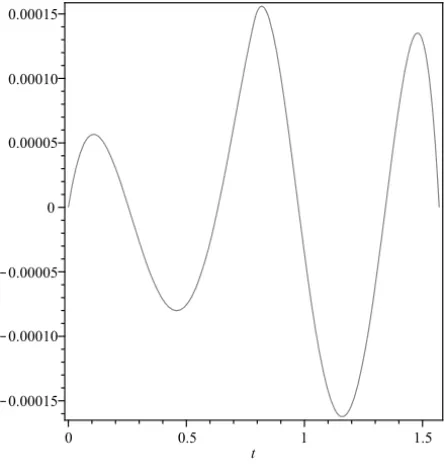
eπ−1 =2.180662822. The graphs ofx1and error function are shown in Figures 4-5.
Figure 4 – Graph of trajectoryx1(t)=x2(t).
Example 3.As a last example, consider a time varying quadratic optimal control problem which is a model of aerospace trajectory control, [20]. The system data is given as follows:
A(t)=
"
2t 1
0 t+1
#
,B(t)=
"
1 2t+2 2t+3
#
,
P(t)=I, Q(t)=1,x0=(1,1)T,
H(t)=K(t)=R(t)=F(t)=0, t∈ [0,4].
Figure 5 – Graph of error.
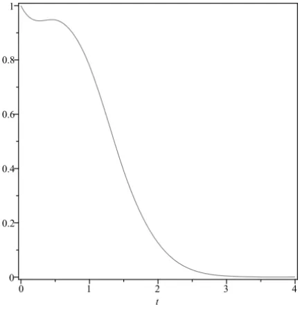
6.573994915. Note that, the five terms of Taylor series ofb21 att = 2 is used instead it. The graphs of x1,x2 and u are shown in figures 6-8. The asymp-totic behaviors of trajectories of the system are discussed in [17] and we see this behaviors in figures.
4 Conclusions
Figure 6 – Graph of trajectoryx1(t).
Figure 8 – Graph of controlu(t).
REFERENCES
[1] A.T. Layton and M. van dePanne, A numerically ecient and stable algorithm for
animating water waves. The visual Computer,18(2002), 41–53.
[2] B. Lang, The synthesis of waveforms using Bézier curves with control point
modulation. The Second CEMS Research Student Conference.
[3] B.P. Molinari, The time-invariant linear-quadratic optimal control problems. Automatica,13(1977), 347–357.
[4] C.H. Chu, C.C.L. Wang and C.R. Tsai,Computer aided geometric design of strip using developable Bézier patches. Computers in Industry,59(6) (2008), 601–611.
[5] D. Burghes and A. Graham, Introduction to control theory including optimal control. John Wiley & Sons (1980).
[6] G. Nürnberger and F. Zeilfelder,Developments in bivariate spline interpolation. Journal of Computational and Applied Mathematics,121(1-2) (2000), 125–152.
[7] G.A. Kurina and R. Marz,On linear-quadratic optimal control problems for time-varying descriptor systems. SIAM J. Control Optim.,42(6) (2004), 2062–2077.
[9] G.E. Farin,Curve and surfaces for computer aided geometric design. Academic Press, New York (1988).
[10] H. Juddu, Spectral method for constrained linear-quadratic optimal control. Mathematics and Computers in Simulation,58(2002), 159–169.
[11] H.R. Marzban and M. Razzaghi, Hybrid functions approach for linearly
con-strained quadratic optimal control problems. Applied Mathematical Modelling,
27(2003), 471–485.
[12] J.V. Beltran and J. Monterde,Bézier solutions of the wave equation. Lecture notes in Computational Sciences,2(2) (2004), 631–640.
[13] J. Zeng, T.W. Sederberg and R.W. Johnson,Least squares methods for solving differential equations using Bézier control points. Appl. Num. Math.,48(2004), 237–252.
[14] K. Harada and E. Nakamae,Application of the Bézier curve to data interpolation. Computer-Aided Design,14(1) (1982), 55–59.
[15] M. Evrenosoglu and S. Somali, Least squares methods for solving singularity perturbed two-points boundary value problems using Bézier control points. Ap-plied Mathematics Letters,21(10) (2008), 1029–1032.
[16] M. Heinkenschloss,A time-domain decomposition iterative method for the solu-tion of distributed linear quadratic optimal control problems. Journal of Compu-tational and Applied Mathematics,173(2005), 169–198.
[17] P. Lu,Closed-form control laws for linear time-varying systems. IEEE Transac-tions on Automatic Control,45(3) (2000), 537–542.
[18] R. Cholewa, A.J. Nowak, R.A. Bialecki and L.C. Wrobel,Cubic Bezier splines
for BEM heat transfer analysis of the 2-D continuous casting problems.
Compu-tational Mechanics,28(2002), 282–290.
[19] R. Winkel, Generalized Bernstein Polynomials and Bézier Curves: An
Appli-cation of Umbral Calculus to Computer Aided Geometric Design. Advances in
Applied Mathematics,27(1) (2001), 51–81.
[20] T. Shu-jun and Z. Wan-xie,Numerical solutions of linear quadratic control for
time-varying systems via symplectic conservative perturbation. Applied
Mathe-matics and Mechanics,28(3) (2007), 277–287.
[21] V. Mehrmann,The autonomous linear quadratic control problems – theory and numerical solution. Lecture Notes in Control and Inform. Sci., 163, Springer-Verlag, Berlin (1991).