ISSN 1549-3644
© 2010 Science Publications
Optimal Boundary Control of the Incompressible
Fluid Problems in Rotation form
Jia Liu
Department of Mathematics and Statistics,
University of West Florida Pensacola, Florida, 32514, USA
Abstract: Problem Statement: We consider the optimal boundary control of the linearized Navier-Stokes problem. Both the Navier-Stokes problem and Oseen problem in rotation form are considered. Approach: We use the Mark and Cell (MAC) discretization method to discretize the optimization problem with linear constraints including the Stokes problem and the Oseen problem in rotation from. Then Reduced Hessian methods are to solve the problem. Results: Numerical experimental results are performed for the boundary optimization problem with the Stokes constraints and Oseen constraints. All the computed solutions and the desired solutions are compared. Conclusions: The proposed reduced Hessian methods have a high accuracy obtaining the optimal boundary conditioning for the Stokes problem and the Oseen problem in rotation form.
Key words: Fluid mechanics, optimization, Navier-stokes, stokes problem, Oseen problem, rotation form, MAC discrcetization, reduced Hessian
INTRODUCTION
We study the incompressible viscous fluid problems with the following form:
u
u (u. )u p f in (0, ]
t
∂ − υ∆ + ∇ + ∇ = Ω× Γ
∂ (1)
.u 0 in (0, ]
∇ = Ω× Γ (2)
u=g in ∂Ω×(0, ]Γ
B (3)
0
u(x,0)=u inΩ (4)
Equation 1-4 is also known as the Navier-Stokes equations. Here Ω is an open set of\d
, where d = 2, or d = 3, with boundary∂Ω, the vari- able u = u(x, t)∈
d
\ is a vector-valued function representing the velocity of the fluid and the scalar function p = p(x, t) ∈ R represents the pressure. The source function f is given onΩ. Here ν > 0 is a given constant called the kine-matic viscosity, which is ν = O (Re−1). Re is the
Reynolds number: VL e= ν
\ , where V denotes the mean velocity and L is the diameter of Ω (Elman et al., 2005). Also, ∆ is the (vector) Laplacian operator in d dimensions, ∇ is the gradient operator and ∇ is the divergence operator. In 3 B is some boundary operator; for example, the Dirichlet boundary condition u = g; or Neumann boundary condition u g
n ∂
=
∂ , where n denotes
the outward-pointing normal to the boundary; or a mixture of the two. Different types of flows may have different types of boundary conditions. If a flow is inside a container, then there must be no flow across the boundary. In this case, we have the boundary condition u. n = 0 on∂Ω. The fundamental principles used to establish these Partial Differential Equations (PDEs) are conservation of mass and conservation of momentum. Equation 1 represents the conservation of momentum and it is called the convection form of the momentum equation. Equation 2 represents the conservation of mass, since for an incompressible and homogeneous fluid the density is constant both with respect to time and the spatial coordinates. Equations 1-4 describe the dynamic behavior of Newtonian fluids, such as water, oil and other liquids.
behavior of the wind flow in the room which correspond the velocity u in the Navier-Stokes equation, which can be controlled by the condition imposed on the boundary. In this project, we are concerned with the boundary control of a flow process governed by the linear zed steady-state Navier-Stokes equations in rotation form.
We use fully implicit time discretization and Picard linearization to obtain a sequence of Oseen problems, i.e., linear problems of the form:
u u (u. )u p f in
α − υ∆ + ∇ = ∇ = Ω (1.5)
.u 0 in
∇ = Ω (1.6)
u=g on ∂Ω
B (1.7)
where, α > 0, with O(1) t α =
δ . Here δt denotes the time step. Equations 5-7 are referred to as the generalized Oseen problem. If α = 0, we have the steady-state problem. If v = 0, we have the Stokes problem.
In this study, we interested in an alternative linearization of the steady-state Navier-Stokes equation. Based on the identity:
1
(u. )u (u.u) ( u) u
2
∇ = ∇ + ∇ × ×
In order to linearize it, we replace u in one place by a known divergence free vector v which can be the solution obtained from the previous Picard iteration. In this case we have:
1
( . )u (u.u) ( u) u
2
ν ∇ ≈ ∇ + ∇ × × (8)
After substituting the right-hand side into (1.5), we find that the corresponding linearized equations have the following form:
u u w u P f in
α − υ∆ + × + ∇ = Ω (9)
.u 0 in
∇ = Ω (10)
u=g on ∂Ω
B (11)
where, P p 1|| u ||2 2 2
= + is the so-called Bernoulli pressure. For the two-dimensional case:
0 w w w 0 × −
where, 1 2
2 1
w
x ∂ν ∂ν = ∇ × ν = − +
∂ν ∂ is a scalar function. In the three-dimensional case, we have:
3 2
3 1
2 1
0 W W
w W 0 W
W W 0
− × = − − (12)
Here, (w1, w2, w3) = w = ∇ × νwhere wi denotes
the ith component of∇ × ν. Assume v = (v1, v2, v3), then
we have the formal expression of w:
1 2 3
i j k
x y x
∂ ∂ ∂
∇ × ν = ∂ ∂ ∂
ν ν ν
(13)
Here the divergence-free vector field v again denotes the approximate velocity from the previous Picard iteration. Note that when the “wind" function v is irrotational(∇ × ν =0) Eq. 9-11 reduce to the Stokes problem. It is not difficult to see that the linearizations 5-7 and 9-11, although both conservative (Olshanskii, 2002), are not mathematically equivalent. The momentum Eq. 9 is called the rotation form. We can see that no first-order terms in the velocities appear in 9 on the other hand, the velocities in the d scalar equations comprising 9 are now coupled due to the presence of the term w × u. The disappearance of the convective terms suggests that the rotation form 9 of the momentum equations may be advantageous over the standard form 5 from the linear solution point of view. This observation was first made by Olshanskii and his co-workers in 2002 (Olshanskii and Reusken, 2002). In their study, they showed the advantages of the rotation form over the standard convection form in several aspects. Benzi and Liu (2007), detailed discussion is provided for the preconditioned iterative methods of the Navier-Stokes problems in rotation form.
Let us consider the area Ω∈\2
, which is a bounded, connected domain with a piecewise smooth boundary ∂Ω. Vector m :∂Ω → 2
\ is the boundary data. Suppose that d∈\2 2
m :∂Ω →\ is the desired velocity, and x is the computed solution of the Navier-Stokes equations, where x = (u, p). In practice, we put a regularization term to the objected function, and β is the regularization parameter. Here 2 n
is a rectangular matrix such that Qx = u. Then the optimal boundary problem governing the linearized rotation form of the Navier-Stokes equation is the following system:
2 2
1 1
min || Qx d || || m ||
2 − + β2
Subject to:
u w u P f in
−υ∆ + × + ∇ = Ω (14)
.u 0 in
∇ = Ω (15)
u=m on∂Ω
B (16)
As we can see, the constraints 14-16 satisfy the rotation form of the steady-state linearized Navier-Stokes equation (which is the steady state Oseen problem in rotation form) with the Dirichlet boundary conditions. Herew= ∇ × ν. Again v is the approximated solution from the previous Picard iteration. If v = 0, we get the (steady-state) Stokes equations.
Discretization: In this study, we consider the Marker-And-Cell (MAC) discretization, which is one of the earliest and most widely used methods for solving fluid flow problems. This scheme is due to Harlow and Welch (1965) and (Fletcher, 1988). The particularity of MAC scheme is the location of the velocity and pressure unknowns. Pressures are defined at the center of each cell and the velocity components are defined at the cell edges (or cell faces in 3D). Figure. 1 shows the staggered grid of MAC discretization. Such an arrangement makes the grid suitable for a control volume discretization.
Fig. 1: Stagger grid of 2D case
We can get the following least squares problem with linear equality constraints based on the MAC discretization:
2 2
1 1
min || Qx d || || m ||
2 − + β2
Subject to: Ax+Pm=0
where, A is the discretization of the Navier-Stokes equation with the following form:
T 1 T 2
1 2
F D B
A D F B
B B C
= −
− −
Here, F = νH, where H is the discretization of Laplacian operator in two dimensions and I is the identity matrix. D is the discretization matrix of the scalar function w= ∇ × ν , the rectangular matrix
T B (i 1, 2)
i = represents the discrete gradient operator while Bi represents its adjoint, the (negative) divergence operator. In order to make the matrix A invertible, we add a stabilization term C = −h2I, where, h = 1 n with n the grid size of the discretization. If D is a zero matrix, then we obtain the coefficient matrix of the Stokes equations. The matrix P is obtained from the discretization of the boundary conditions.
From (Fletcher, 1988), we can discretize the second order derivatives using the following approximation:
2 1
nx 1 1 0 2 2 2
u 1
(u 2u u )
x h +
∂
≅ − +
∂
Also we can assume u1 + u0 = 2m1 where u0 is the
ghost point of outside the boundary. Then we have: 2
1
nx 1 1 1 2 2 2
u 1
(u 3u 3m )
x h +
∂ = − +
∂
Hence we have: 2
1
nx 1 1 1
2 2 2 2
u 1 2
(u 3u ) m
x h + h
∂ ≅ − +
After discretization, the coefficient Puy matrix on the boundary function of vector u (where u = (u, v)) along the y direction is of the form:
2 2 2 2 0 0 h 2 0 0 h Puy 2 0 0 h
0 0 0
0 0 0
= " " " " " "
Similarly, we can obtain the form of the matrix Pux which is the boundary condition of the vector u along the x direction:
2 2 2 1 0 0 h 1 0 0 h Pux 1 0 0 h
0 0 0
0 0 0
= " " " " " "
Similar analysis for the boundary condition of vector v along the x and y direction. We can get the other two matrices Pvx, Pvy. For the 2D problems, we obtain the boundary coefficient matrix as follows:
Pux Puy 0 0
P
0 0 Pvx Pvy
MATERIALS AND METHODS
The resulting optimization problem written in constrained form is the following:
2 2
1 1
min || Qx d || || m ||
2 − + β2
Subject to: Ax+Pm=0
Now introducing the lagrangian:
2 2 T
1 1
(x, m, ) min || Qx d || || m || (Ax Pm) 0
2 2
λ = − + β +λ + =
L
A necessary condition for an optimal solution of our problem is:
T T
x=Q (Qx−d)+A λ= 0
L (3.17)
T m= β + λm P 0
L (3.18)
Ax Pm 0
λ= + =
L (3.19)
Using (19) to eliminate x and then (17) to eliminate λ yields a nonlinear least squares data fitting problem. See more details in (Stephen and Wright, 1999). Since 17-19 are linear equations; we just need to solve these equations directly, which lead to the following Karush-CKuhn-CTucker (KKT) system:
T
kkt
x Q b
H m 0
0 = −
λ
Where:
T T
T
kkt
Q Q 0 A
H 0 I P
A P 0
= β
Notice that Hkkt is the large, sparse, linear system
on which the present study concentrates.
Next, we show how to get the reduce Hessian matrix and how to solve it. Based on 17-19, we proceed to eliminate x, then λ and finally solve for m:
1
X= −A Pm− (20)
T T
A Q Q(b− Qx)
λ = − − (21)
T T T 1 T 1 T
( Iβ +P A Q QA P)m− − = −P A Q d− (22)
Which leads to the equations:
T T T 1 T 1 T
( Iβ +P A Q QA P)m− − = −P A Q d− (23)
Or:
T 1 T red
H m= −P A Q d− (24)
Where: T
red
H = β +I J J (25)
1
Here Hred is the reduced Hessian. Since β > 0, the
reduced Hessian becomes a symmetric positive definite matrix. Therefore, for the solution of (3.24) we may use a PCG (preconditioned Conjugate Gradient) other iterative methods to solve the system. Furthermore, the matrix J is large and dense, the evaluation of Jv proceeds by first forming Pv, then solve the forward problem to obtain A−1 v and finally multiplying the result by Q. Each evaluation of Hredv in the PCG step
involves the following steps:
• w1 = Pv
• Solve Aw2 = w1
• w3 = QTQw2
• Solve ATw4 = w3
• w = PTw4
Therefore each Matrix-vector product of Hredv
requires the solution of one for-ward problem which to solve the equation Ax = b and one adjoint problem AT x = b to a high degree of accuracy, so it is very expensive. We may consider to use iterative methods to calculate the forward problem like Gener-alized Minimal Residual (GMRES) method or PCG method. However the convergence of those methods without preconditioning may be slow. Therefore how to choose a fast and efficient preconditioner is a one problem. Furthermore the choice to the convergence tolerance of the inner iteration (for the preconditioning steps) and outer iteration (PCG steps) can be essential to the rate of the convergence of the problem. Simoncini and Szyld (2003) for more details.
RESULTS
We give some numerical experiments based on the algorithm we have discussed. First we need to show that we have the right format of the boundary conditions. All results were computed in MATLAB 7.1.0 on one processor of an AMD Opteron with 32 GB of memory.
Let us choose u = cos (2 xπ ) cos (2 yπ ), v = cos (2 xπ ) cos (2 yπ ), p = sin (2 xπ ) sin (2 yπ ) which are the analytical solutions of the Navier-Stokes equations. We plug in the analytical solution to the Navier-Stokes equation to get the right hand side b and also we calculate the value of Ax + Pm. Here x = (u, v, p)T. The norm of the difference between these two is the error.
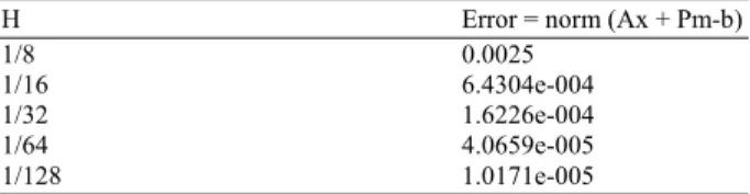
As we know, the error of MAC discretization is of O(h2). Therefore, as the grid size doubles, the error should be decreased by1
4. Table 1 shows that as the
grid size increases twice from 64-128, the error decreases from 4.0659e-005-1.0171e-005, which shows that the discretized boundary matrix P is the correct discretization of the boundary conditions.
Next, we did two different experiments to test the algorithms. We have chosen two different desired solutions: one satisfies the linearized rotation form of the Navier-Stokes equation and the other satisfies the Stokes equation (in this case,∇ × =u 0). Consider the area Ω = [0, 1]×[0, 1] and a MAC scheme on staggered grids for velocity and pressure. We setw= ∇ ×u, where u = (v1, v2), with v1= −x 2y; v2=2x+y We can see in this case u satisfies the Navier-Stokes equation. Also we choose another vector u′, where u′ = (v′1, v′2), with
v′1 = −y, v′2 = x in this case, u′ satisfies the Stokes
equation.
Figure 2 shows the desired flow and computed flow for the Stoke problems. The left two graphs present the desired Stokes flow (upper image) and computed flow (lower image). We can see for the Stokes case, the computed solution is almost the same as the desired solution. The flows inside the area and boundary conditions are perfectly match. Figure 2b shows the boundary conditions for the computed Stokes flow, which are the x boundary function of the vector u at the left side, x boundary function of the vector u at the right side, y boundary function of the vector u on the top side, y boundary function of the vector u at the bottom side; x boundary function of the vector v at the left side, x boundary function of the vector v at the left side, y boundary function of the vector v on the top side, y boundary function of the vector v at the bottom side. Figure 3 shows the desired flow and computed flow for the Oseen problems in rotation form. In this case that w ≠ 0. We use 0.1 for the viscosity. We can see from the graphs the computed solution (lower image) is very close to the desired solution (upper image) around the boundary, however, inside the domain, there is some difference. This might due to the linearization and discretization errors and complexity of the Oseen problem especially in the rotation form. Again Fig. 3b presents the boundary conditions of the computed Oseen flow in rotation form in x and y directions. Notice that in all these experiments, we use
Table 1: Error test for the boundary matrix P
H Error = norm (Ax + Pm-b)
1/8 0.0025
1/16 6.4304e-004
1/32 1.6226e-004
1/64 4.0659e-005
(b)
Fig. 2: Stokes flow (a) Desired (upper image) and computed (lower image) Stokes flows (b) Boundary condition of the computed Stokes flow
(b)
Fig. 3: Oseen flow in rotation form (a) Desired and computed Oseen flow; (b) Boundary condition of the computed Oseen flow in rotation form
Table 2: number of iterations of the CG method: The stokes problem
H iteration numbers
1/8 12
1/16 21
1/32 30
1/64 37
1/128 47
Table 3: number of iterations of the CG method: The Oseen problem in rotation form
H ν = 0:1 ν = 0:01 ν = 0:001
1/8 23 31 28
1/16 29 24 33
1/32 38 31 23
1/64 49 37 27
1/128 59 44 33
direct method to solve all the linear systems in the reduced Hessian method. We can replace the direct methods by the inexact method like PCG or Preconditioned GMRES methods to solve the problem more efficiently and the results will not be affected.
DISCUSSION
In these numerical experiments, we use Conjugate Gradients methods to solve the reduce Hessian matrix. Table 2 and Table 3 show the number of the iterations of the CG iterative methods for the Stokes flow and the Oseen flow in rotation form. Here we used direct methods to calculate the forward problem and its adjoint problem. As we can see, the number of the iterations increases as the grid size increases for both the Stokes and Oseen flows. Therefore a preconditioning is a must. Benzi and Liu (2007), we have a detailed discussion about the Hermitian and Skew-Hermitian preconditioned iteration method for the Stokes equations and Oseen equations in rotation form.
CONCLUSIONS
Skew-Hermitian (HSH) preconditioned GMRES methods for the Oseen problem in rotation form and excellent results are given in the study. Therefore, we can consider to use PCG to solve the linear system in the reduce Hessian methods if we have the Stokes flow, or we can switch to the HSS preconditioned GM-RES methods if we have the Oseen flow in rotation form. In the future, we can consider to use different convergence tolerance to accelerate the convergence of linear system solvers. Furthermore, even though we only discuss the 2D case in the study, we can obtain the similar results for the 3D case.
ACKNOWLEDGMENT
The researcher would like to thank Eldad Haber for helpful instructions and suggestions.
REFERENCES
Benzi, M. and J. Liu, 2007. An efficient solver for the incompressible navier-stokes equations in rotation form. SIAM. J. Sci. Comput., 29: 1959-1981. DOI: 10.1137/060658825
Elman, H., D. Silvester and A. Wathen, 2005. Finite Elements and FastIterative Solvers with Applications in Incompressible Fluid Dynamics. Oxford University Press, ISBN: 019852868X, pp: 313.
Fletcher, C.A.J., 1991. Computational Techniques for Fluid Dynamics. 2nd Edn., Springer-Verlag, ISBN: 0-38755-3058-4, pp: 58.
Haber, E. and U.M. Ascher, 2001. Preconditioned all-at-once methods for large, sparse parameter estimation problems. Inv. Prob., 17. DOI: 10.1088/0266-5611/17/6/319
Olshanskii, M.A. and A. Reusken, 2002. Navier--stokes equations in rotation form: A robust multigrid solver for the velocity problem. SIAM. J. Sci.
Comput., 23:1683-1706. DOI: 10.1137/S1064827500374881
Simoncini, V. and D.B. Szyld, 2003. Theory of inexact krylov subspace methods and applications to scientific computing. SIAM. J. Sci. Comput., 25: 454-477. DOI: 10.1137/S1064827502406415 Stephen, J.N. and J. Wright, 1999. Numerical