Mat. Res. vol.13 número2

*e-mail: [email protected]

Mathematical Model for Timber Decay in Contact with the

Ground Adjusted for the State of São Paulo, Brazil

Roberto Ramos de Freitas*, Julio Cesar Molina, Carlito Calil Júnior

School of Engineering of São Carlos, University of São Paulo – USP,

Av. Trabalhador Sãocarlense, 400, CEP 13566-590 São Carlos, SP, Brazil

Received: July 20, 2009; Revised: May 5, 2010

At this moment, the environmental sustainability has been incorporated to all branches of activity more and more; timber seems to be the best alternative in civil construction. Nevertheless, for a correct and better usage of timber as a structural material, it is necessary to have a higher degree of knowledge not only of the structural mechanical behavior, but also about its durability and service life. With help from mathematical models the

service life of the timber structures can be foreseen, by obtaining the “Climate Indices”, that show comparatively

among the studied regions, which ones have a higher or lesser propensity of being attacked by fungi. In this paper, utilizing climatologic data from several cities of the State of São Paulo - Brazil was determined through numerical analysis and statistics, the simplification of one aggressive model to timber in contact with the ground, being this model adjusted to the State of São Paulo. The simplified model of timber degradation can be used to quantity the effect of the environment in the process of decay for the regional climatic conditions.

Keywords: timber, decay model, durability

1. Introduction

There’s no doubt that wood is one of the most versatile materials that nature puts at the disposal of humankind. Wood has been used for millions of years to fulfill the needs that come from a society that is each time thirstier for new sources of energy and raw materials.

With many possibilities to utilize the wood, both in civil construction and in industry, round timbers and ties (stakes, shoring, poles and columns, etc.), represent some of the most efficient uses of our natural forest resources, demanding a minimum of processing between the harvesting of the tree and selling the structural commodity. Because these products are somewhat cheap to produce, compared to gluelam, steel and concrete articles, they are more often

than not used far and wide in the United States1_.

No material is inherently durable due to the environmental and micro-structural interactions consequently, the material properties change as time passes by, admitting that the limit of use has been reached, when its properties decay, under certain conditions of usage, up to a point that to keep on using this material is considered unsafe

or anti-economical2_.

Life service gives the measurement of time of a product and its materials, in which normal usage conditions (that is, if it’s not put into stressful conditions beyond acceptable limits) can last conserving its own capacities (service, output, etc) and its own behavior, in a

pre-established standard level3_.

2. Decay

The biological nature of the wood makes it susceptible to the aggressions of fungi and insects, however the drying and the preservation of a side, and the association to other materials in the places of constructions that are more vulnerable to attacks than others, make the timber structures as durable as steel or concrete, since its

conception respects certain rules of protection of the material4_.

The main groups of xylophagan organisms are the bacteria, fungi,

insects, clams, crustaceans5_{, being that the decay fungi are responsible}

for deep alterations in the physical and mechanical properties of the wood, due to gradual destruction of the molecules that constitute its cellular walls5,6_.

The decay affects initially the stiffness, the ability of the material to resist impacts generally, being followed by reduction of the resistance the static bending, and finally all the properties of resistance

of the wood seriously are reduced7_.

After having established the layer of fungi, the speed of growth of these is dependant primarily of the humidity and temperature, Figure 1a. The conditions of growth of the fungi vary a lot from one species to another, but as a general rule, it has been observed that for temperatures below 5 °C the fungi had lived dormant, while for

temperatures above 65 °C these will be dead in a few hours8_.

As for the humidity, the speed of growth of the fungi is extremely low for values of humidity below the fiber saturation point, Figure 1b, the lesser humidity in which the fungi grow that has been observed is 19%, and the superior limit corresponds to 80% humidity, where the cell cavities are saturated8_.

3. Models of Decay

A model for the decay of parts in contact with the ground was proposed based in small monitored stakes for more than 30 years in

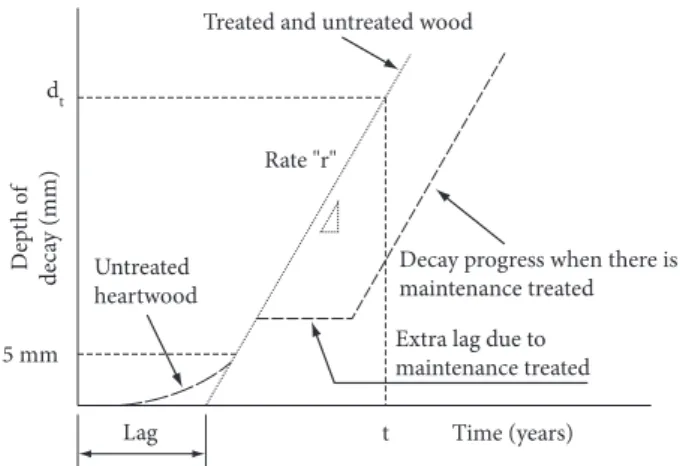
Australia9_{. Such model considers that a time (lag) for the beginning}

of the decay process exists, which after the beginning evolves in a speed (reason “r”) constant, being able to occur a new initial time and stop the decay with maintenance accomplishment, Figure 2.

Figure 1. Functions idealized for two parameters of decay8_.

Figure 2. Relationship of idealized decay9_.

g T T se T C

T

mean mean mean

me

(

)

= − + × < ≤ °

− + ×

1 0 2 5 20

25 1 4 ,

, _aanseT_mean> °C

 

 ₂₀ (Equation 4)

As for the influence of the types of wood present in one pole, it is admitted the project considered in Figure 3, where the rates of

decay are shown schematically for the types of wood9_{. The list of}

used abbreviations is presented in the Appendix 1.

To determine the initial time for the installation of the decay process (lag) and the decay rate (r), the following equations and the parameters of Table 1 are adopted.

•฀ Outer฀heartwood

run heart stake, , = ×A Iig

(Equation 5)

•฀ Corewood

lag_{un core stake, ,} =0 3, ×lag_{un heart stake, ,}

(Equation 6)

r_{un core stake, ,} = ×3 r_{un heart stake, ,}

(Equation 7)

•฀ Sapwood

lag_{un sap stake, ,} =0 5, ×lag_{un heart dc, , 4,stake}

(Equation 8)

r_{un sap stake, ,} = ×2 r_{un heart dc, , 4,stake (Equation 9)}

3.1. Being

lag_{un, heart, dc4, stake}: the initial time of decay for the external heartwood species of durability class 4;

r_{un, heart, dc4, stake}: decay rate for the external heartwood species of durability class 4;

4. Studied Region

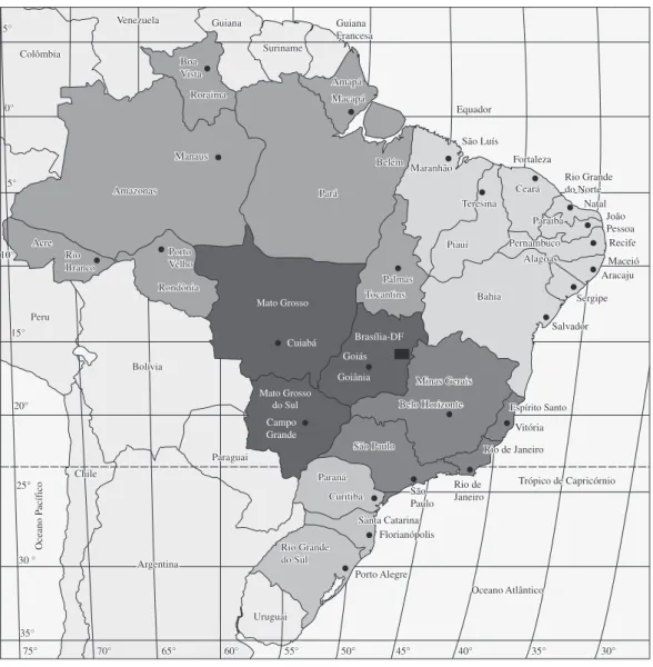
São Paulo is one of the states of Brazil, being located approximately between the longitudes 44° and 53° W and latitudes 20° and 25° S, a small part is below of the Capricorn Tropic (23° 27’ 09” S). Thus most of the State of São Paulo this located in a tropical region. Figure 4 shows the localization of the State of São Paulo in Brazil.

The State of São Paulo has a large extent of mountainous areas of altitude, where the rain is sufficiently mild and thus it can generally be classified as tropical of altitude, where the rain is abundant, over

all in the station stowage, making the climate humid tropical10_.

According to the climatic classification of Koeppen, the State of São Paulo encloses six distinct climatic types, all corresponding to the humid climates. The type that corresponds to the biggest area is the

Table 1. Parameters of decay for external not treated heartwood9_.

Durability class (AS 5604-2005)

A Initial time

lag_{un, heart, stake} (years)

Class 1 0.20 6

Class 2 0.55 4

Class 3 0.80 2

Class 4 1.85 1

Figure 4. Localization of São Paulo State.

Table 2. Statistics of the climatic data.

Statistics Temperature

(°C)

Annual Precipitation (mm)

N_dm – dry months

Mean 22.6 1446 0.8

Minimum 15.1 1165 0.0

Maximum 25.7 2514 1.9

Amplitude 10.6 1349 1.9

Table 3. Statistics of the climatologic data.

Statistics I_ig

Mean 2.48

Minimum 2.04

Maximum 2.5

Amplitude 0.81

Considering the classes of aggressiveness form the initial model17_,

Table 4 shows the distribution of cities in relation to this classification.

Table 4. Representative climatic Index for four classes of aggressiveness.

Region of decay Representative I_ig Number of cities

A 0.5 0

B 1.5 0

C 2.5 49

determination of the values of I_ig and I_{ig; simplified} was carried through only for the stations that possessed a minimum period of reading, until the moment of the attainment of the data, of at least 5 years, thus 11 weather forecast stations had been discarded of the study. This measurement contributes so that little representative values are not obtained, in function of annual variations of the climate. Table 2 shows the descriptive statistics of the climatic data of the studied cities.

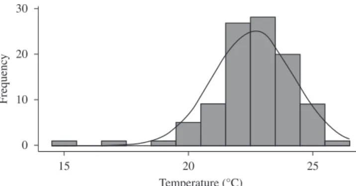
Figures 5 to 7 show the distributions of absolute frequency for the data of Temperature, Annual Precipitation and Dry Months. The normal distribution curve is shown next to the histogram.

5. Application of Leicester’s Model

Table 3 shows the descriptive statistics for the obtained values

with the application of the climatologic data to Leicester’s model9_.

Considering the classes of aggressiveness form the initial

model17_{, Table 4 shows the distribution of cities in relation to this}

classification.

Table 5 shows the descriptive statistics for the population variables of I_{ig < 2.50} e I_{ig > 2.50}.

Intending to verify if the cities classified by the decay regions according to Table 5 have different temperature populations, precipitation and dry months, the F-test of variables is carried through (using Snedecor’s distribution), dividing them into two populations; cities with I_ig smaller than 2.50 (I_{ig < 2.50}) and cities with I_ig greater than 2.50 (I_{ig > 2.50}).

Adopting a significant level of 5% (α = 0.05) for the F-test we

have that:

•฀ F-Test฀for฀temperature

H₀: the variance of temperatures for I_{ig < 2.50} and I_{ig > 2.50} are equal. H₁: the variance of temperatures for I_{ig < 2.50} and I_{ig > 2.50} are not equal. Fobtained: 2.845 Fcritic: 1.596 P-Value: 0.0001

Conclusion: reject H0

•฀ F-Test฀for฀precipitation

H₀: the variance of precipitations of I_{ig < 2.50} and I_{ig > 2.50} are equal. H₁: the variance of precipitations of I_{ig < 2.50} and I_{ig > 2.50} are not equal. Fobtained: 3.307 Fcritic: 1.604 P-Value: 0.000025

Conclusion: reject H0 •฀ F-Test฀for฀dry฀months

H₀: the variance of dry months of I

ig < .2.50 and Iig > 2.50 are equal. H₁: the variance of dry months of I

ig < 2.50 and Iig > 2.50 are not equal. Fobtained: 1.220 Fcritic: 1.604 P-Value: 0.244

Conclusion: not reject H0

Figure 5. Absolute frequency histogram of the average temperatures for the cities of São Paulo State.

Figure 6. Absolute frequency histogram of the annual precipitations for the cities of São Paulo State.

Figure 7. Absolute frequency histogram of the dry months for the cities of São Paulo State.

Table 5. Descriptive statistics for the population variables of I_ig.

Statistics Temperature

(°C)

Precipitation (mm)

N_dm – dry months

– I_{ig < 2.50} I_{ig > 2.50} I_{ig < 2.50} I_{ig > 2.50} I_{ig < 2.50} I_{ig > 2.50}

Mean 21.5 23.6 1405 1483 0.87 0.80

Minimum 15.1 21.5 1165 1174 0.25 0.00

It can be concluded that the variable N_dm (dry months) is not for this set of data in analysis_, it isn’t a variable of significant contribution for determining I_ig.

6. Proposition of Model

The simplification proposed is the withdrawal of the variable

“N_dm - dry months”, which is the hardest to attain. This proposal is

justified, since carrying through the F-test for this variable for the populations of I_ig < 2.50 and I_ig > 2.50, did not give statistical evidence of difference between this data set.

The simplification is initiated only with the withdrawal of the

variable N_dm of the model. The model to be used initially is given

bellow:

6.1. Leicester’s simplified model

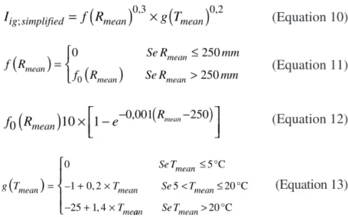
Iig simplified; f Rmean g Tmean

, ,

=

(

)

0 3×

(

)

0 2

(Equation 10)

f R

Se R mm

f R Se R mm

mean mean mean mean

(

)



₍

₎

 = ≤ > 0 250 250 0 (Equation 11)

f R_mean e Rmean

0

(

)

10× −_1 −0 001,

(

−250

)

_ (Equation 12)

g T

Se T

T Se T

T mean mean mean mean me

(

)

= ≤

+ × < ≤

− + ×

0 5

1 0 2 5 20

25 1 4

°C

°C – ,

, _aan Se T_mean> 

 

 20 °C

(Equation 13)

Table 6 compares the descriptic statistics of I_ig e I_ig; simplified. Figure 8 compares the dispersion of the values of I_ig and I_{ig; simplified}. A positive displacement (increase of the values) of the population of data as well as of the average can be observed.

To verify proposal of the simplification done, it is necessary to observe if there is a correlation between the values of the current model and the simplified model. Figures 9 and 10 show the regression and the residues of the regression for I_ig and I_{ig; simplified}, respectively.

The value of r2 _{- coefficient of determination for this regression is}

of 83.3%.

From Figure 10 it is observed that the correlation between I_ig and I_{ig; simplified} does not present independence of errors in function of I_{ig; simplified}. This characteristic can be explained considering that for the

exact same value of the reduction factor (1 – N_dm/6), the difference

between the value of I_ig and I_{ig; simplified} increases proportionally to the second variable.

Adopting the same classification of aggressiveness already used9_,

Table 7 shows the distribution of I_{ig; simplified}.

Table 8 shows the descriptive statistics for the climatologic indices of the populations of I_ig; simplified.

The F-test is carried through to identify if it is possible to consider that the two populations I_ig and I_{ig; simplified} are equal. Thus, for α = 0.5 we have:

•฀ F-Test฀I_ig e I_{ig; simplified}

H₀: the variances of I

ig and Iig; simplified are equal. H₁: the variances of I_ig and I_{ig; simplified} are not equal.

Fobtained: 1.087 Fcritic: 1.389 P-Value: 0.338

Conclusion: not reject H0

From the test above it is possible to verify statistical evidences that the populations of I_ig and I_{ig; simplified}are equal.

As previously, the F-test is carried through between the populations of temperature and precipitation, verifying if the populations of these parameters differ in I_{ig; simplified}, dividing them again in two populations; cities with I_{ig; simplified} smaller than 2.50 (I_{ig; simplified < 2.50}) and cities with I_{ig; simplified} greater than 2.50 (I_{ig; simplified > 2.50}). This way, for a level of significance of 5% (= the 0.05) we have that:

•฀ F-Test฀for฀temperature

H₀: the variance of temperatures of I_{ig; simplified < 2.50} and I_{ig; simplified > 2.50} are equal.

H₁: the variance of temperatures of I_{ig; simplified < 2.50} and I_{ig; simplified > 2.50} are not equal.

Fobtained: 2.517 Fcritic: 1.639 P-Value: 0.0001

Conclusion: reject H0 •฀ F-Test฀for฀precipitation

H₀: the variance of precipitations of I

ig; simplified < 2.50 and Iig; simplified > 2.50

are equal.

H₁: the variance of precipitations of I_{ig; simplified < 2.50} and I_{ig; simplified > 2.50} are not equal.

Fobtained: 2.062 Fcritic: 1.766 P-Value: 0.019

Conclusion: reject H0

There are no statistical evidence that the temperature populations and precipitation are equal for the populations I_{ig; simplified < 2.50} and I_{ig; simplified > 2.50}.

One฀concludes฀that฀the฀withdrawal฀of฀the฀N_dm variable of the model proposed by Leicester, did not influence the variables temperature and precipitation, in determination of the aggressiveness index, since the population of the values of these variables, are still distant for I_{ig; simplified < 2.50} and I_{ig; simplified > 2.50}, for the studied data set.

6.2. Analysis of regressions

Completing a regression between the values of I_ig and I_{ig; simplified}

for the ten most aggressive cities according to I_ig, a low value of the

determination coefficient, r2 _{= 36.6% is obtained, Figure 11.}

However, the regression between the values of I_ig and I_{ig; simplified} for the ten less aggressive cites according to I_ig, a high value of

determination coefficient, r2 _{= 95.5% is obtained, Figure 12.}

The equation of the straight line it is given by:

y=ax+b (Equation 14)

So that the values of the x coordinate are equal to the ones of the y coordinate, it is necessary that the linear coefficient (a) be null, and that the value of angular coefficient (b) be equal to 1, as the Equation 15.

y= + ×0 1 x (Equation 15)

The greater the value of the linear coefficient (a) and that of the angular coefficient (b) in module, greater the distance the straight line is from the identity (y = x).

Table 9 compares the values of the linear and angular coefficients of the regression carried through previously. It is verified that the values of the coefficient is very close to the values for the identity

only for regression to the smaller I_ig values.

Withdrawing the N_dm variable (dry months), the populations of

Table 9. Coeficient values of the regressions I_ig × I_{ig; simplified}.

Regression Coeficient r2

(%)

Linear (a) Angular (b)

I_ig × I_{ig; simplified} (Figure 9) 0.208034 0.874643 83.3

I_ig × I_{ig; simplified} (greater I_ig) 1.73412 0.3621805 36.6

I_ig × I_{ig; simplified} (smallerI_ig) - 0.0849705 1.00447 95.5

Table 7. Representative climatic index for four classes of aggressiveness.

Decay region Representative I_{ig; simplified} Number of cities

A 0.5 0

B 1.5 0

C 2.5 28

D 3.0 74

Table 8. Descriptive statistics of the parameters of the populations of I_{ig; simplified}.

Statistics Temperature

(°C)

Precipitation (mm)

– I_{ig; simplified < 2.50} I_{ig; simplified > 2.50} I_{ig; simplified < 2.50} I_{ig; simplified > 2.50}

Mean 20.8 23.3 1393 1465

Minimum 15.1 21.3 1167 1165

Maximum 22.2 25.7 1726 2514

Figure 11. Regression between I_ig and I_{ig; simplified} for the cities of the greatest values of I_ig.

values of I_ig.

Table 6. Descriptic statistics of I_ig e I_{ig; simplified}.

Statistics I_ig I_{ig; simplified}

Mean 2.48 2.60

Minimum 2.04 2.12

Maximum 2.85 2.86

Amplitude 0.81 0.74

Figure 9. Regression I_ig × I_{ig; simplified}.

Temperature, Precipitation and Dry Months, for the populations of I_{ig < 2.50} and I_{ig > 2.50}, it was concluded that it does not exist statistical evidences of difference of these two populations for the variable Dry Months.

Carrying through the simplification of the initial model, and

determining the values of I_{ig, simplified}, the population of these values

with the population of I_ig can be compared, not getting statistical evidences that indicate difference in these two populations of climatic indices.

The best regression between I_ig and I_{ig; simplified} is the one carried through between the ten smaller values of I_ig and its respective I_{ig; simplified}, this being the closest to the straight line identity. Through this regression it was possible to propose an adjusted final model of

climatic index of timber decay in contact with the ground, the I_LL-SP.

This model is adjusted to the data of the State of São Paulo, which does

not possess the necessity of the N_dm variable (dry months) with the

attainment of approximately the same obtained initial values through Leicester’s Model. Thus two alternative models to the initial one are possible, the one of Leicester: the I_{ig; simplified} and the I_LL-SP.

For the analyzed data the simplification of Leicester’s model can be considered as adequate.

Acknowledgements

We thank IAC - Agronomic Institute of Campinas, pertaining agency to the Secretary of Agriculture and Supplying of the State of São Paulo, for the supply of the climatic data.

References

1. Wolfe RW. Round timbers and ties. In: United States Department of Agriculture - USDA. Wood handbook: wood as an engineering material. Madison: USDA; 1999. p. 18.1-18.9. General technical report FPL - 113.

2. Mehta PK and Monteiro PJM. Estruturas de concreto. São Paulo: Pini; 1994.

3.฀ Manzin฀E฀and฀Vezzoli฀CO.฀Desenvolvimento de produtos sustentáveis.

São Paulo: Edusp; 2005.

4.฀ Fusco฀PB.฀Os฀caminhos฀da฀evolução฀da฀engenharia฀das฀madeiras.฀In:฀

Anais do 3º Encontro Brasileiro de Madeira e Estruturas de Madeira; 1989; São Carlos - SP, Brasil. São Carlos: LaMEM/EESC/USP; 1989. p. 7-18.

5. Cavalcante MS. Deterioração biológica e preservação de madeiras. São Paulo: IPT; 1982.

6. Instituto de Pesquisas Tecnológicas – IPT. Biodeterioração de madeiras em edificações. São Paulo; 2001.

7. Highley TL. Biodeterioration of wood. In: United States Department of Agriculture – USDA. Wood handbook. Madison: Forest Products Laboratory; 1999. p. 13.1-13.5.

8. Leicester RH. Engineered durability for timber construction. Highett:

CSIRO;฀2001.฀12฀p.

9. Leicester RH, Wang CH, Nguyen MN, Foliente GC and Mckenzie C. An engineering model for the decay of timber in ground contact. In:

Proceedings 34º Annual Meeting of The International Research Group On Wood Preservation; 2003; Brisbane-Austrália, Stockholm, Suécia; 2003. 21 p.

10.฀ Paes฀A,฀ Camargo฀ DE,฀ Pinto฀ HS,฀ Brunini฀ O,฀ Pedro฀ Jr.฀ MJ,฀ Ortolani฀

AA, Alfonsi RR. Conceituação. [cited 2007 Jul. 24]. Available from: http://www.ciagro.sp.gov.br/clima. .

value the dispersion of data around the regression of the straight line t is high.

Appling Equation 16, which is the regression for the tem smallest values of I_ig and its respective I_{ig; simplified}, to all values of I_{ig; simplified}, I_ig’ for all the cities is obtained.

I_ig’ =1 00447, ×I_{ig simplified;} −0 0849705, (Equation 16)

Subtracting the value of Iig’ from Iig the Error (e) of the estimate is gotten, as Equation 17. Through these the value of the Mean Error

(E_m) of the estimate is determined, Equation 18.

E=Iig−IIg’ (Equation 17)

E I I

n m ig Ig i l n =∑ − = ’ (Equation 18)

The value of the Mean Error (E_m) is of -0.0438074. Adding this

value to the Equation 16, the final model adjusted is obtained to the data of the State of São Paulo, which will be called Climatic Index of the State of São Paulo for timber decay in contact with the ground.

I_{LL SP−} =1 00447, ×I_{ig simplified;} −0 0849705, −0 0438074, (Equation 19)

ILL SP− =1 00447, ×Iig simplified; −0 12878, (Equation 20)

Thus two models are proposed, the simplified model (Equation 21) which was shown to have small variation from the initial Leicester’s model, and the model adjusted for the State of São Paulo (Equation 22).

I_{ig simplified;} =f R

(

_mean

)

0 3, ×g T

(

_mean

)

0 2, (Equation 21)

I_LL =1 00447, ×f R

(

_media

)

0 3, ×g T

(

_media

)

0 2, −0 12878, (Equation 22)

f R

Se R mm

f R Se R mm

media mean media mean

(

)



₍

₎

 = ≤ > 0 250 250 0 (Equation 23)

f R_media e Rmedia

0

0 001 250

10 1

(

)

   = × − −, ( − ) (Equation 24) gT SeT C

T Se T C

media

media

media media

(

)

=

≤ °

− + × < ≤ °

− +

0 5

1 0 2 5 20

25 1 4

,

, ×× > °

  



 _{T SeT C}

media media 20

(Equation 25)

7. Conclusions

The possibility of a greater and better rational use of the timber necessarily passes through the attainment of a better knowledge of how this material behaves with elapsing of the time.

The models of timber degradation represent a form to quantify the effect of the environment in the process of decay for the regional climatic conditions.

Appling the initial model of degradation of timber in contact

I_{ig < 2,50} Value de I_ig smaller than 2,50 I_{ig > 2,50} Value de I_ig greater than 2,50

I_{ig; simplified} Simplified Climatic Index for timber decay in contact with the ground I_{ig; simplified < 2,50} Simplified Climatic Index smaller than 2,50

I_{ig; simplified > 2,50} Simplified Climatic Index greater than 2,50