Persistence criteria for susceptibility genes for schizophrenia: a discussion from an evolutionary viewpoint.

(1)

Schizophrenia: a Discussion from an Evolutionary

Viewpoint

Nagafumi Doi1*, Yoko Hoshi2, Masanari Itokawa3, Chie Usui4, Takeo Yoshikawa5, Hirokazu Tachikawa1,6 1Department of Psychiatry, Ibaraki Prefectural Tomobe Hospital, Kasama-shi, Ibaraki, Japan,2Integrated Neuroscience Research Team, Tokyo Institute of Psychiatry, Kamikitazawa, Setagaya-ku, Tokyo, Japan,3Schizophrenia Research Project, Tokyo Institute of Psychiatry, Kamikitazawa, Setagaya-ku, Tokyo, Japan,4Department of Psychiatry, Faculty of Medicine, Juntendo University, Tokyo, Japan,5Laboratory for Molecular Psychiatry, RIKEN Brain Science Institute, Hirosawa, Wako, Saitama, Japan, 6Department of Psychiatry, Graduate School of Comprehensive Human Science, Tsukuba University, Tsukuba, Ibaraki, Japan

Abstract

Background:The central paradox of schizophrenia genetics is that susceptibility genes are preserved in the human gene-pool against a strong negative selection pressure. Substantial evidence of epidemiology suggests that nuclear susceptibility genes, if present, should be sustained by mutation-selection balance without heterozygote advantage. Therefore, putative nuclear susceptibility genes for schizophrenia should meet special conditions for the persistence of the disease as well as the condition of bearing a positive association with the disease.

Methodology/Principal Findings:We deduced two criteria that every nuclear susceptibility gene for schizophrenia should fulfill for the persistence of the disease under general assumptions of the multifactorial threshold model. The first criterion demands an upper limit of the case-control difference of the allele frequencies, which is determined by the mutation rate at the locus, and the prevalence and the selection coefficient of the disease. The second criterion demands an upper limit of odds ratio for a given allele frequency in the unaffected population. When we examined the top 30 genes at SZGene and the recently reported common variants on chromosome 6p with the criteria using the epidemiological data in a large-sampled Finnish cohort study, it was suggested that most of these are unlikely to confer susceptibility to schizophrenia. The criteria predict that the common disease/common variant hypothesis is unlikely to fit schizophrenia and that nuclear susceptibility genes of moderate effects for schizophrenia, if present, are limited to ‘rare variants’, ‘very common variants’, or variants with exceptionally high mutation rates.

Conclusions/Significance:If we assume the nuclear DNA model for schizophrenia, it should have many susceptibility genes of exceptionally high mutation rates; alternatively, it should have many disease-associated resistance genes of standard mutation rates on different chromosomes. On the other hand, the epidemiological data show that pathogenic genes, if located in the mitochondrial DNA, could persist through sex-related mechanisms.

Citation:Doi N, Hoshi Y, Itokawa M, Usui C, Yoshikawa T, et al. (2009) Persistence Criteria for Susceptibility Genes for Schizophrenia: a Discussion from an Evolutionary Viewpoint. PLoS ONE 4(11): e7799. doi:10.1371/journal.pone.0007799

Editor:Amanda Ewart Toland, Ohio State University Medical Center, United States of America

ReceivedMarch 17, 2009;AcceptedAugust 22, 2009;PublishedNovember 11, 2009

Copyright:ß2009 Doi et al. This is an open-access article distributed under the terms of the Creative Commons Attribution License, which permits unrestricted use, distribution, and reproduction in any medium, provided the original author and source are credited.

Funding:The authors have no support or funding to report.

Competing Interests:The authors have declared that no competing interests exist. * E-mail: n.doi@pref.ibaraki.lg.jp

Introduction

While the development of genomics technology, coupled with sophisticated designs of linkage and association studies, is opening up new opportunities of genetics research of complex diseases, it may still be important to view the study of human disease from an epidemiological perspective [1]. The aim of this paper is to view the recent findings of molecular genetics of schizophrenia (SZ) and to examine the peculiarity of the genetic basis of SZ from an epidemiological standpoint.

SZ is a common deleterious psychosis with high heritability (80– 85%), which manifests typically in adolescence or early adulthood [2]. SZ crosses all cultures at a relatively high prevalence (0.5–1%) [2,3], and seems to be an ancient condition. The incidence of SZ, at the macro-level, varies within narrow limits [3], and appears to

be stable across generations in several countries [4,5]. On the other hand, it has been well documented that patients with SZ have a remarkably reduced reproductive fitness (0.3–0.8 as compared with the value in the normal population; the reduction is more pronounced in male patients) [6–17]. Then how can a pathogenic gene predisposing to SZ persist against a strong negative selection pressure? This ‘persistence problem’ has puzzled scientists for long years [18–20].

From an evolutionary viewpoint, four explanations are possible [18,20]: (i) mutation-selection balance, (ii) heterozygote advantage (balancing selection), (iii) negative frequency-dependent selection, and (iv) ancestral neutrality.

(2)

were close to zero. Because the effective population size in ancient times might be much smaller than now, pathogenic but neutral alleles could have been fixed by genetic drift. While this hypothesis explains that SZ has not been extinct in the long human history, ancestral neutrality itself provides no explanation for the apparently stable incidence of the disease across generations today; although ‘ancestral neutrality’ might be plausible, it needs another mechanism to account for the persistence of the disease in modern environments, where the effective population size has been expanded and the influence of negative selection pressure may be much stronger than ever before.

‘Negative frequency-dependent selection’ explains the persis-tence only when the fitness of the affected individuals increases as the prevalence in the general population decreases, which seems not to be the case with SZ.

‘Heterozygote advantage’ assumes that the susceptibility alleles increase the fitness of the unaffected gene carriers, thereby sustaining the gene frequencies. This line of explanations include: (i) physiological advantage (resistance to shock, infections, and poor nutrition etc.) [21], (ii) creative intelligence [22] or a higher trait creativity including ‘everyday creativity’ [23], and (iii) a higher sexual activity and/or attractiveness [24]. Since the unaffected siblings of the patients are expected to share pathogenic genes, those hypotheses need two lines of confirmation: (a) that the unaffected siblings of the patients have such advantages, and (b) that such advantages really contribute to sufficiently increase their reproductive fitness.

Some of those hypotheses seem to gain the confirmation (a). For example, Kinney et al. [23], in a well designed and methodolog-ically sophisticated study, showed that an advantage of everyday creativity was linked to a subtle clinical picture (schizotypal signs) in a non-psychotic sample of SZ offspring.

However, those hypotheses lack the confirmation (b) in the nuclear DNA (ncDNA) model; those hypotheses, although theoretically plausible and fascinating, have not been supported by most epidemiological studies, which show a decreased reproductive fitness of the unaffected siblings of the patients [14,16,17,25–28]. Haukka et al. [17], in a large-sampled cohort study, showed an increased reproductive fitness of unaffectedfemale siblings of patients with SZ. However, this statistically higher fertility of the female siblings (1.033) was not large enough to compensate for the gene loss due to the decreased reproductive fitness of the patients (0.346) and their male siblings (0.950) in the ncDNA model. More recently, Svensson et al. [29], in a large-sampled three generation cohort study, did not find an increased fertility among parents, siblings or offspring of patients with SZ (except for a slightly and not significantly increased fertility,1.02 in healthy female siblings).

Thus, if we assume the ncDNA model for SZ, the remaining possibility is the mechanism of mutation-selection balance without heterozygote advantage. (Keller and Miller [20] comprehensively discussed this problem, leading to a similar conclusion. The difference from our argument is that Keller and Miller overlooked the possibility of ‘ancestral heterozygote advantage’ and discussed against ancestral neutrality.) Therefore, loss of the risk alleles due to the decreased reproductive fitness of the patients should be balanced byde novomutation in each risk locus. A nuclear gene for SZ should meet this ‘persistence condition’ in addition to the condition of bearing a significant association with SZ. This simple and essential principle has been overlooked in SZ genetics.

Here we deduce two criteria that a nuclear susceptibility gene for SZ should fulfill for the persistence of the disease under general assumptions of multifactorial threshold model, and present their implications for genetic association studies and genetic models for SZ using the epidemiological data in a large-sampled Finish cohort study.

Results

We deduced a series of criteria (‘persistence criteria’) that every nuclear susceptibility gene for SZ should fulfill for the persistence of the disease against a strong negative selection pressure. While the association condition between a risk allele and the disease demands the lower limit zero of the case-control difference of the allele frequencies (d~j jMA{j jMU;j jMA= allele frequency in the affected population,j jMU= allele frequency in the unaffected population), the first criterion demands an upper limitvof the difference, which is determined by the prevalence of the disease (p), the selection coefficient of the disease (s), and the mutation rate at the locus (m). Thus we have:0vdvv, wherevis defined

by v~ð1{spÞm

1{p

ð Þsp. The second criterion derived from the first gives an upper limit of odds ratio (OR) of the pathogenic allele for a given allele frequency in the unaffected population. Since the association condition demands 1vOR, we have:

1vORv1z v

M

j jU 1{v{j jMU

for0vj jMUv1{v.

Since mutation rates of the putative risk loci are unknown, three versions of the persistence criteria are shown in theTable 1. The stronger version corresponds to the lowest mutation rate m~1:48|10{6_{per locus per generation (for mutation rates see}

section 4 in Method) while the weaker version corresponds to the highest1:48|10{4

and the standard version corresponds to the average1:48|10{5

.

Because the estimated value ofv1:76|10{4_v_v_v₁_:₇₆_|₁₀{2

is remarkably small, the persistence criteria is very demanding. Among the 36 single nucleotide polymorphisms (SNPs) at

Table 1.Three versions of persistence criteria.

Stronger version Standard version Weaker version

m 1:48|10{6 _1:48_|₁₀{5 _1:48_|₁₀{4

n 1:76|10{4 _1:76_|₁₀{3 _1:76_|₁₀{2

Criterion A 0vj jMA{j jMUv0:000176 0vj jMA{j jMUv0:00176 0vj jMA{j jMUv0:0176

Criterion B For0vj jMUv0:999824,

ORv1z 0:000176

M

j jU0:999824{j jMU

For0vj jMUv0:99824,

ORv1z 0:00176

M

j jU0:99824{j jMU

For0vj jMUv0:9824,

ORv1z 0:0176

M

j jU 0:9824{j jMU

M

j jA: Allele frequency in the affected population,

M

j jU: Allele frequency in the unaffected population.

(3)

SZGene [30] that have significantPvalues (Pv0:05) in the meta-analyses, only 9 SNPs fulfill the weaker version of the criterion A (Table 2): the G-allele of rs1801028 (DRD2), the C-allele of rs1327175 (PLXNA2), the A-allele of rs9922369 (RPGRIP1L), the A-allele of rs2391191 (DAOA), the C-allele of rs35753505 (NRG1), the G-allele of rs4680 (COMT), the T-allele of rs737865 (COMT), the T-allele of rs1011313 (DTNBP1), and the A allele of rs3213207 (DTNBP1). None of these SNPs meet the standard version of the criteria. Therefore, these SNPs cannot meet the persistence criteria unless they have the highest mutation rate.

None of the recently reported common SNPs on chromosome 6p22.1 associated with SZ [31] meet the weaker version of the criterion A (Table 3). Therefore, those common variants are unlikely to confer susceptibility to SZ unless they have exception-ally high mutation rates. The best imputed SNP in a recent genome-wide association study (GWAS) [32], which reached a genome-wide significance (the A-allele of rs3130297 on chromo-some 6p;Pv4:69|10{7_{), does not meet the weaker version of} the criterion A (d.0.02; see Table 1 in the paper [32]). Therefore, this SNP is unlikely to contribute to risk of SZ unless it has an exceptionally high mutation rate. Similarly, none of the top 100 SNPs in a recent GWAS [32] fulfill the weaker version of the criterion A (see Table 1 in the paper [33]).

Three of the 7 common SNPs associated with SZ in the latest GWAS [34] clearly do not meet the weaker version of the criterion B. The remaining 4 SNPs may fulfill the weaker version but not the standard version (see Table 1 in the paper [34]). Therefore, these 4 SNPs are unlikely to confer susceptibility to SZ unless they have the highest mutation rate.

ORfor a given allele frequency in the unaffected population and the range of allele frequency in the unaffected population for a given OR calculated with the criterion B under three levels of mutation rate are presented in theTables 4and5, respectively. Required sample sizes for association studies for a single allele and for GWAS are shown in the Tables 6and 7, respectively. Powers of association study for a single allele and of GWAS with given sample sizes are shown inTables 8and9. Surprisingly, the power of GWAS with a sample size as large as 100,000 case-control pairs to detect a common variant of a mutation rate not higher than the average is almost zero (Table 9).

Discussion

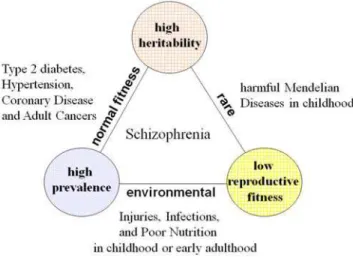
The three epidemiological properties- high heritability, high prevalence and low reproductive fitness- form a Devil’s triangle; any combination of the two tends to exclude the third, and in this triangle most diseases vanish except for SZ (Figure 1). Diseases with high heritability and high prevalence such as type 2 diabetes and adult cancers are late-onset diseases and may show almost normal reproductive fitness. Diseases with high prevalence and low reproductive fitness such as poor nutrition, severe injuries and infections in childhood or early adulthood are mainly due to the environmental factors. Diseases with low reproductive fitness and high heritability such as most harmful Mendelian diseases in childhood are rare. From this point of view, SZ, a disease with those three properties, may be unique and peculiar.

This peculiar epidemiological characteristic of the disease may put SZ in a unique position among the common diseases with genetic bases; it might be afforded, not surprisingly, by a unique and peculiar genetic basis. The persistence criteria, although with notable limitations such as assuming a large effective population size at equilibrium and random mating (seeMethod), may approxi-mately describe the peculiarity of the genetic basis for SZ. Let us examine the peculiarity of SZ genetics with the persistence criteria.

1. The CD/CV hypothesis is unlikely to fit SZ

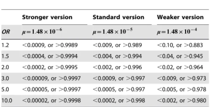
First, we can see that the common disease/common variant (CD/CV) hypothesis [35], [36] is unlikely to fit SZ. The standard version of the criterion B implies that theOR of every risk allele with a population frequency between 0.05 and 0.95 is less than 1.04 (Table 4). The weaker version implies that theORof every risk allele with a population frequency between 0.04 and 0.945 is less than 1.50 (Table 5). Therefore, given the standard range of mutation rate (1:48|10{6_v_m_v₁_:₄₈_|₁₀{4_{), the effect size and} the population frequency of a nuclear risk variant for SZ cannot simultaneously satisfy the expectations in the CD/CV hypothesis, in which common alleles at a handful of loci are assumed to interact to cause a common disease.

2. Nuclear risk variant for SZ of moderate effects, if present, should be either rare or very common

As previously mentioned, the persistence criteria argue against the CD/CV hypothesis. However, it does not necessarily mean that only the multiple rare variant model [37,38] fits SZ. The standard version of the criterion B implies that the frequency of a pathogenic variant of a moderate effect (ORw3:0) in the ncDNA, if present, should be either very low in the affected population (j jMAvj jMUzvv0:0027) or very high in the normal population (j jMUw0:997) (Table 5). The weaker version implies that the frequency of a nuclear susceptibility variant of a moderate effect should be either low (j jMAvj jMUzvv0:027) or high (j jMUw0:973) (Table 5). Thus we can see that given the standard range of mutation rate nuclear genes of moderate effects for SZ, if present, are limited to either ‘rare variants’ or ‘very common variants’.

‘Very common variants’ for a deleterious disease might seem at odds; how could variants associated with a deleterious disease ever have become so common in spite of the enormous cost the species should pay for?

Given a much smaller effective population size in ancient times, ‘ancestral heterozygote advantage’ and genetic drift, coupled with less pronounced reproductive disadvantage of the ancestral patients, could provide an explanation. Although the ancestral patients might also show a reduced reproductive fitness, the reproductive disadvantage could have been less pronounced in ancient environments because many patients could have children before the onset of their illness; individuals in ancient times might have their first children at a lower age (15–20 years = adolescence) than individuals in modern times (25–30 years; seesection 4 in Method). Advantages of the unaffected siblings such as everyday creativity could better work to increase their reproductive fitness in ancient times than today. In addition, the effective population size might be much smaller in ancient times. Thus, susceptibility genes could have been neutral or almost neutral (selection coefficient

v 1

4Ne

;Ne= the effective population size) in ancient times. Then,

pathogenic but neutral or almost neutral genes in ancient environ-ments could be fixed at a high frequency close to 1 by genetic drift (because the effective population size might be much smaller and the effects of genetic drift might be predominant in ancient times) and can be sustained by mutation-selection balance today.

(4)

Table 2.Top polymorphisms in Top 30 genes at SZGene [30] (August 10, 2009).

Genes and SNPs Allele (minor/major) _{j jj}jM_A_{(sample size)} _j_{j jj}M_U_{(sample size)} P-value OR d

1. DISC1

rs3737597 A*/G 0.07881 (N = 1,142) 0.05231 (N = 1,797) 0.000245 1.4 0.0265

2. SLC18A1

rs2270641 C*/A 0.31818 (N = 759) 0.28022 (N = 885) 0.0614 1.63 0.0380

3. GABRB2_{: none}

4.DRD2

rs1079597 (Taql-B) A/G* 0.81325 (N = 830) 0.78273 (N = 803) 0.0229 1.37 0.0315

rs6277 C*/T 0.50412 (N = 3,159) 0.46080 (N = 4,043) 0.00000199 1.37 0.0433

rs1801028 G*/C 0.03337 (N = 6,173) 0.02643 (N = 7,908) 0.00323 1.22 0.0069

rs6275 T*/C 0.33862 (N = 2,903) 0.31100 (N = 3,336) 0.00198 1.15 0.0276

5. GWA 10q26.13

rs17101921 A*/G 0.06667 (N = 7,447) 0.04318 (N = 13,039) 0.00000000 1.28 0.0235

6. AKT1

rs3803300 A*/G 0.33705 (N = 2,645) 0.31460 (N = 2,999) 0.0257 1.05 0.0225

7. GRIN2B

rs1019385 T/G* 0.56041 (N = 687) 0.48846 (N = 650) 0.00050 1.33 0.0720

rs7301328 G*/C 0.44256 (N = 1,088) 0.40845 (N = 994) 0.0862 1.17 0.0341

8. DGCR2

rs2073776 A*/G 0.39824 (N = 2,727) 0.37117 (N = 3,004) 0.010 1.14 0.0271

9.PLXNA2

rs1327175 G/C* 0.92840 (N = 1,711) 0.91243 (N = 1,770) 0.043 1.32 0.0160

10.RPGRIP1L

rs9922369 A*/G 0.04221 (N = 5,474) 0.03437 (N = 10,823) 0.0014 1.3 0.0078

11. TPH1

rs1800532 A*/C 0.50726 (N = 1,239) 0.45052 (N = 1,708) 0.0000799 1.25 0.0567

12. DRD4

120-bp TR S/L* 0.80421 (N = 1,236) 0.76397 (N = 1,199) 0.00380 1.23 0.0402

rs1800955 C*/T 0.41964 (N = 2,128) 0.39823 (N = 2,206) 0.0653 1.13 0.0231

13.DAOA

rs3916971 T/C* 0.56220 (N = 844) 0.52115 (N = 922) 0.045 1.19 0.0411

rs778294 T/C* 0.78375 (N = 6,444) 0.77250 (N = 7,677) 0.069 1.04 0.0113

rs2391191 (M15) A*/G 0.50063 (N = 8,692) 0.48820 (N = 10,680) 0.029 1.01 0.0124

14._{GWA 11p14.1}

rs1602565 C*/T 0.14240 (N = 7,170) 0.12112 (N = 12,611) 0.00000001 1.16 0.0213

15. DRD1: none

16. HTR2A

rs6311 A/*G 0.44847 (N = 2,678) 0.41784 (N = 2,964) 0.00457 1.16 0.0306

17. RELN

rs7341475 A/G* 0.85477 (N = 3,009) 0.82569 (N = 7,045) 0.00000283 1.14 0.0291

18. APOE _e2/3/4* _{0.12061 (N = 2,931)} _{0.10257 (N = 5,065)} _0.0135 _1.09 _0.0181

19.NRG1

rs2439272 A/G* 0.64395 (N = 2,935) 0.61284 (N = 2,797) 0.00101 1.18 0.0312

rs35753505 C*/T 0.42656 (N = 9.082) 0.41024 (N = 9,921) 0.00658 1.04 0.0163

rs473376 G*/A 0.17252 (N = 3,701) 0.14611 (N = 4,589) 0.0000435 1.08 0.0264

20. IL1B

rs1143634 T/C* 0.83626 (N = 1,197) 0.81951 (N = 1,435) 0.0564 1.06 0.0167

21. MTHFR

rs1801133 T*/C 0.34340 (N = 4,055) 0.31491 (N = 5,535) 0.000135 1.14 0.0341

22._COMT

(5)

unclear, these reports seem to be in line with the predictions of the persistence criteria. However, no reports have identified ‘very common variants’ associated with SZ to date.

3. The largest GWAS to date lacks the power to identify a common variant of the average mutation rate

The persistence criteria predict that common pathogenic variants, if present, can have only tiny effects. Nevertheless,

Table 3.Common variants on chromosome 6p22.1 associated with SZ [31].

rs ID

Allele (minor/

major) j_{j jj}M_A _j_{j jj}M_U P-value OR d

rs6904071 A/G* 0.834 0.814 1:78|10{8 _1.14–1.25 _0.020

rs926300 T/A* 0.834 0.814 1:06|10{8 _1.14–1.26 _0.020

rs6913660 A/C* 0.836 0.816 2:36|10{8 _1.13–1.25 _0.020

rs13219181 G/A* 0.837 0.817 1:29|10{8 _1.14–1.26 _0.020

rs13194053 C/T* 0.838 0.818 9:54|10{9 _1.14–1.28 _0.020

rs3800307 A/T* 0.817 0.795 4:35|10{8 _1.13–1.27 _0.022

rs3800316 C/A* 0.771 0.743 3:81|10{8 _1.13–1.20 _0.028

*_{alleles associated with schizophrenia,}

d~j jMA{j jMU.

doi:10.1371/journal.pone.0007799.t003

Genes and SNPs Allele (minor/major) _{j jj}jM

A(sample size) jj jjMU(sample size) P-value OR d

rs737865 C/T* 0.69100 (N = 6,288) 0.67468 (N = 9,131) 0.00320 0.95 0.0163

23. HP

Hp1/2 1/2* 0.62296 (N = 1,346) 0.59291 (N = 2,018) 0.0443 1.14 0.0300

24. DAO

rs2111902 G*/T 0.39094 (N = 2,517) 0.36807 (N = 2,960) 0.0455 1.07 0.0229

rs3741775 C/G* 0.57980 (N = 2,514) 0.55542 (N = 2,959) 0.0218 1.09 0.0244

rs3918346 A*/G 0.35145 (N = 2,521) 0.32957 (N = 2,966) 0.0463 1.05 0.0219

rs4623951 C/T* 0.78378 (N = 1,509) 0.67883 (N = 1,521) 0.0915 1.14 0.0249

25. TP53

rs1042522 C*/G 0.39880 (N = 1,418) 0.36879 (N = 1,410) 0.0675 1.13 0.0300

26. ZNF804A

rs1344706 G/T* 0.59933 (N = 7,183) 0.58402 (N = 12,663) 0.0129 1.12 0.0191

27. GWA 16p13.12

rs71992086 T*/A 0.27009 (N = 7,179) 0.24558 (N = 12,623) 0.00000039 1.12 0.0245

28.DTNBP1

rs1011313 T*/C 0.11722 (N = 7,695) 0.10562 (N = 7,276) 0.00652 1.08 0.0116

rs1018381 T/*C 0.09666 (N = 4,940) 0.08727 (N = 4,927) 0.0763 1.11 0.0094

rs2619538(SNPA) T*/A 0.49804 (N = 5,598) 0.47671 (N = 5,862) 0.00758 1 0.0213

rs3213207(P1635) G/A* 0.90835 (N = 8,472) 0.89811 (N = 8,391) 0.00694 1.08 0.0102

29. OPCML

rs3016384 T/C* 0.53882 (N = 7,187) 0.51744 (N = 12,675) 0.000264 1.08 0.0214

30. RGS4

rs2661319 (SNP16) A/G* 0.49313 (N = 8,010) 0.47446 (N = 9,183) 0.00249 1.08 0.0187

*_{alleles associated with SZ,}

d~j jMA{j jMU.

SNPs withP-value less than 0.1 are listed. doi:10.1371/journal.pone.0007799.t002

Table 2.Cont.

Table 4.OR_{vs. allele frequency in the unaffected population.}

jM

j jjU m~~1:48||10{{6

m~~1:48||10{{5

m~~1:48||10{{4

0.001 ,1.18 ,2.77 ,17.9

0.01 ,1.02 ,1.18 ,2.81

0.02 ,1.009 ,1.09 ,1.92

0.05 ,1.004 ,1.04 ,1.38

0.1 ,1.002 ,1.02 ,1.20

0.3 ,1.0009 ,1.009 ,1.09

0.5 ,1.0008 ,1.008 ,1.08

0.7 ,1.0009 ,1.009 ,1.09

0.9 ,1.002 ,1.02 ,1.24

0.95 ,1.004 ,1.04 ,1.58

0.98 ,1.009 ,1.10 ,8.49

0.99 ,1.02 ,1.22 -*

0.999 ,1.22 -* -*

*The upper limit ofORis dependent on the allele frequency in the affected population:ORv1z v

1{j jMA

M

j jA{v

:

(6)

identification of common pathogenic variants would be much more difficult than previously thought. The persistence criteria imply thatthe sample size required in an association study for SZ with a given power depends on the mutation rate at the putative risk locus as well as the population frequency of the putative pathogenic variant. Thus we can see that an enormous sample size is required to identify a common pathogenic variant of a standard mutation rate (Table 6and7). For example, more than the half of all the SZ patients in the world (w3:76|107_{; we assume here a total human population of}

6:0|109_{and a prevalence of 1%) and the same number of control} subjects should be recruited to the association study to identify a common variant (population frequency: 0.1–0.9) at a putative risk locus of a mutation rate1:48|10{6_{with a power 0.95 (}_{Table 6}_). When the mutation rate is assumed to be average, more than one million case-control pairs are required to identify a common variant in a GWAS with a power 0.8 (Table 7).

Because the sample size of the largest GWAS and association studies to date is far less than 50,000 case-control pairs (Tables 10 and 11), those studies lack the power to identify a common pathogenic variant of the average mutation rate (Tables 8and9). The power of the GWAS to identify common variants of the highest mutation rate has merely reached to the level of,0.1 for the past two years (Tables 7and9).

4. Too strong association implies that the variants may not confer susceptibility

Since the criterion A demands a small upper limit of the case-control difference of the allele frequencies, too strong association imply that the allele may not confer susceptibility to SZ. Especially, common variants associated with SZ in an association study with a sample size smaller than the estimations in the Tables 6and7are unlikely to contribute to risk of SZ.

Let us consider the cases of the SNPs in theTable 2. Among the 36 SNPs that have significantPvalues in the meta-analyses at Table 6.Required sample size in an association study for a

common variant.

x~~_{j jj}_jM Azj jjjMU

₂ _v

~

~1_:76||10{{4

v~~1_:76||10{{3

v~~1_:76||10{{2

0.1 or 0.9

1{b~0.95 w3:76|107 _w_3:76_|₁₀5 _w_3:76_|₁₀3

1{b~0.80 w2:27|107 _w2:27_|₁₀5 _w2:27_|₁₀3

1{b~0.10 w1:34|106 _w1:34_|₁₀4 _.₁₃₄

0.2 or 0.8

1{b~0.95 w6:69|107 _w6:69_|₁₀5 _w_6:69_|₁₀3

1{b~0.80 w4:04|107 _w4:04_|₁₀5 _w4:04_|₁₀3

1{b~0.10 w2:38|106 _w_2:38_|₁₀4 _.₂₃₈

0.3 or 0.7

1{b~0.95 w8:78|107 _w8:78_|₁₀5 _w8:78_|₁₀3

1{b~0.80 w5:31|107 _w5:31_|₁₀5 _w5:31_|₁₀3

1{b~0.10 w3:13|106 _w_3:13_|₁₀4 _.₃₁₃

0.4 or 0.6

1{b~0.95 w1:00|108 _w1:00_|₁₀6 _w1:00_|₁₀4

1{b~0.80 w6:07|107 _w_6:07_|₁₀5 _w6:07_|₁₀3

1{b~0.10 w3:58|106 _w_3:58_|₁₀4 _.₃₅₈

0.5

1{b~0.95 w1:04|108 _w1:04_|₁₀6 _w1:04_|₁₀4

1{b~0.80 w6:32|107 _w_6:32_|₁₀5 _w_6:32_|₁₀3

1{b~0.10 w3:73|106 _w_3:73_|₁₀4 _.₃₇₃

Samples:Ncases+Ncontrols,a~0.05,1{b~0.95, 0.8, 0.1.

N% z0:05zz0:05

d

2

xð1{xÞw 3:60

v 2

xð1{xÞfor1{b~0.95.

N% z0:05 zz0:2

d 2

xð1{xÞw 2:80

v 2

N% z0:05 zz0:9

d 2

xð1{xÞw 0:68

v 2

Table 5.Allele frequency in the unaffected population vs.OR_.

OR m~~1:48||10{{6

m~~1:48||10{{5

m~~1:48||10{{4

1.2 ,0.0009, or.0.9989 ,0.009, or.0.989 ,0.10, or.0.883 1.5 ,0.0004, or.0.9994 ,0.004, or.0.994 ,0.04, or.0.945

2.0 ,0.0002, or.0.9995 ,0.002, or.0.996 ,0.02, or.0.964

3.0 ,0.00009, or.0.9997 ,0.0009, or.0.997 ,0.009, or.0.973 5.0 ,0.00005, or.0.9997 ,0.0005, or.0.997 ,0.005, or.0.978

10.0 ,0.00002, or.0.9998 ,0.0002, or.0.998 ,0.002, or.0.980

Table 7.Required sample size in GWAS for SZ.

x~~ _j_{j jj}M Azjj jjMU

₂ _v

~

~1_:76||10{{4

v~~1_:76||10{{3

v~~1_:76||10{{2

0.1 or 0.9

1{b~0.95 w1:33|108 _w_1:33_|₁₀6 _w_1:33_|₁₀4

1{b~0.80 w1:04|108 _w_1:04_|₁₀6 _w_1:04_|₁₀4

1{b~0.10 w4:35|107 _w4:35_|₁₀5 _w4:35_|₁₀3

0.2 or 0.8

1{b~0.95 w2:38|108 _w_2:38_|₁₀6 _w_2:38_|₁₀4

1{b~0.80 w1:85|108 _w1:85_|₁₀6 _w1:85_|₁₀4

1{b~0.10 w7:73|107 _w7:73_|₁₀5 _w7:73_|₁₀3

0.3 or 0.7

1{b~0.95 w3:12|108 _w_3:12_|₁₀6 _w_3:12_|₁₀4

1{b~0.80 w2:43|108 _w2:43_|₁₀6 _w2:43_|₁₀4

1{b~0.10 w1:01|108 _w1:01_|₁₀6 _w1:01_|₁₀4

0.4 or 0.6

1{b~0.95 w3:57|108 _w3:57_|₁₀6 _w3:57_|₁₀4

1{b~0.80 w2:77|108 _w2:77_|₁₀6 _w2:77_|₁₀4

1{b~0.10 w1:16|108 _w_1:16_|₁₀6 _w_1:16_|₁₀4

0.5

1{b~0.95 w3:72|108 _w3:72_|₁₀6 _w3:72_|₁₀4

1{b~0.80 w2:89|108 w2:89|106 w2:89|104

1{b~0.10 w1:20|108 _w_1:20_|₁₀6 _w_1:20_|₁₀4

Samples:N_cases₊N_controls,_a~2:5|10{7_,₁_{_b_~_{0.95, 0.8, 0.1.}

N% z0:00000025 zz0:05

d

2

xð1{xÞw 6:79

v 2

N% z0:00000025 zz0:2

d

2

xð1{xÞw 5:99

v 2

N% z0:00000025 zz0:9

d

2

xð1{xÞw 3:87

v 2

(7)

SZGene, 9 SNPs can fulfill the weaker version of the criteria only if they have the highest mutation rate. However, the remaining 27 SNPs cannot meet the criteria unless they have exceptionally high mutation rates (w1:48|10{4_{). For example, the G-allele of} rs1019385 (GRIN2B), which shows P= 0.0005 in the meta-analysis, cannot meet the criteria unless the mutation rate of the

locus is higher than 6:05|10{4_~ð1{pÞsp

1{sp |0:072. However, this value may be too high as compared with the upper limit of mutation rates on autosomes and X chromosome (1:48|10{4_). Alternatively, this SNP must be a protective or resistance gene (i.e. a gene elevating the carrier’s fitness by reducing the liability to the disease as well as the severity of the disease).

It should be noted that high mutation rates (m§2:3*4:4|10{4₎ have been reported on human Y chromosome [52]. Therefore, common variants on Y chromosome or on the pseudoautosomal regions of X chromosome where abundant mutation could be supplied by synapsis and crossing over with Y chromosome, could meet the persistence criteria. In this case, however, putative risk loci would be highly polymorphic because of abundant mutation supply. Common CNVs also could meet the criteria, if they have extremely high mutation rates (m§1:48|10{4_).

In the future, with expansion of the sample size and pooled data, GWAS and meta-analyses may identify many more variants associated with SZ. While some of them may fulfill the persistence criteria, the others do not. Then, associated variants that do not fulfill the persistence criteria should be either susceptibility genes of exceptionally high mutation rates or resistance genes of standard mutation rates. Thus, in the near future, we are to choose one of the alternative cases: (1) a case in which SZ should have many

susceptibility genes with tiny effects of exceptionally high mutation rates, or (2) a case in which SZ should have many resistance genes of standard mutation rates on different chromosomes associated with SZ itself. This may be the most peculiar aspect of SZ genetics that the persistence criteria predict.

Table 8.Power of association study for a single variant.

x~~_{j jj}_jM_Az_{j jj}_jM_U₂ _v

~

~1_:76||10{{4 _v ~

~1_:76||10{{3 _v ~

~1_:76||10{{2

0.1 or 0.9

N= 10,000 ,0.03 ,0.09 ,1

N_{= 20,000} _,_0.04 _,_0.13 _,₁

N= 50,000 ,0.04 ,0.27 ,1

0.2 or 0.8

N_{= 10,000} _,_0.03 _,_0.07 _,_0.999

N= 20,000 ,0.03 ,0.10 ,1

N= 50,000 ,0.04 ,0.17 ,1

0.3 or 0.7

N= 10,000 ,0.03 ,0.07 ,0.99

N= 20,000 ,0.03 ,0.08 ,0.9999

N_{= 50,000} _,_0.04 _,_0.14 _,₁

0.4 or 0.6

N= 10,000 ,0.03 ,0.06 ,0.95

N_{= 20,000} _,_0.03 _,_0.08 _,_0.9999

N= 50,000 ,0.04 ,0.13 ,1

0.5

N_{= 10,000} _,_0.03 _,_0.05 _,_0.95

N= 20,000 ,0.03 ,0.08 ,0.999

N= 50,000 ,0.04 ,0.13 ,1

Samples:Ncases+Ncontrols,a~0.05.

Power:1{bvW

ffiffiffiffiffiffiffiffiffiffiffiffiffiffiffiffiffiffiffiffiffiffiffiffiffiffiffiffiffiffiffiffiffi_N xð1{xÞv{z

0:05

r

%W

ffiffiffiffiffiffiffiffiffiffiffiffiffiffiffiffiffi_N xð1{xÞ r

v{1:96

.

Table 9.Power of GWAS for SZ.

x~~_j_{j jj}M_Az_j_{j jj}M_U₂ _v

~

~1:76||10{{4 _v ~

~1:76||10{{3 _v ~

~1:76||10{{2

0.1 or 0.9

N_{= 10,000} _,_0.000001 _,_0.00001 _,_0.76

N= 50,000 ,0.000001 ,0.0001 ,1

N= 100,000 ,0.000001 ,0.001 ,1 0.2 or 0.8

N= 10,000 ,0.000001 ,0.00001 ,0.23

N= 50,000 ,0.000001 ,0.0001 ,1

N_{= 100,000} _,_0.000001 _,_0.001 _,₁

0.3 or 0.7

N= 10,000 ,0.000001 ,0.00001 ,0.10

N_{= 50,000} _,_0.000001 _,_0.0001 _,_0.9999

N= 100,000 ,0.000001 ,0.0001 ,1 0.4 or 0.6

N= 10,000 ,0.000001 ,0.00001 ,0.07

N= 50,000 ,0.000001 ,0.0001 ,0.999

N= 100,000 ,0.000001 ,0.0001 ,1 0.5

N= 10,000 ,0.000001 ,0.00001 ,0.06

N= 50,000 ,0.000001 ,0.0001 ,0.999

N= 100,000 ,0.000001 ,0.0001 ,1

Samples:Ncases+Ncontrols,a~2:5|10{7_.

Power:1{bvW

ffiffiffiffiffiffiffiffiffiffiffiffiffiffiffiffiffiffiffiffiffiffiffiffiffiffiffiffiffiffiffiffiffiffiffiffiffiffiffiffiffiffiffi N

xð1{xÞv{z

0:00000025

r

%W

ffiffiffiffiffiffiffiffiffiffiffiffiffiffiffiffiffi N xð1{xÞ r

v{5:15

.

Figure 1. Devil’s triangle of high heritability, high prevalence and low reproductive fitness.The three epidemiological properties-high heritability, properties-high prevalence and low fitness- form a Devil’s triangle; any combination of the two tends to exclude the third. In this triangle most diseases vanish except for schizophrenia.

(8)

Table 10.Pooled sample sizes in association studies for top 30 genes at SZGene [30].

Candidates Cases (Caucasian) Controls (Caucasian) Cases (Total) Controls (Total)

1. DISC1 5,762 7,449 8,006 9,697

2. SLC18A1 673 1,283 1,346 1,948

3. GABRB2 1,625 1,788 2,887 2,873

4. DRD2 8,291 11,436 10,915 14,259

5. GWA 10q26.13 5,666 11,174 7,531 13,039

6. AKT1 2,798 3,274 4,248 4,662

7. GRIN2B 737 704 1,765 1,680

8. DGCR2 1,195 1,384 5,549 5,771

9. PLXNA2 705 739 1,401 1,685

10. RPGRIP1L 5,526 10,969 5,526 10,969

11. TPH1 905 1,845 1,960 3,068

12. DRD4 4,027 5,684 7,070 8,307

13. DAOA 5,562 7,290 9,424 11,555

14. GWA 11p14.1 5,526 10,969 7,308 12,834

15. DRD1 1,303 1,917 1,502 2,213

16. HTR2A 8,226 8,809 10,907 11,284

17. RELN 3,705 8,301 4,711 9,340

18. APOE 2,624 4,646 4,693 7247

19. NRG1 7,069 9,494 12,995 15,091

20. IL1B 1,420 2,373 2,161 3,096

21. MTHFR 3,411 5,037 4,752 6,320

22. COMT 12,640 22,644 18,140 29,065

23. HP 1,300 1,966 1,863 2,492

24. DAO 1,953 2,427 3,120 3,585

25. TP53 383 443 1,418 1,410

26. ZNF804A 5,526 10,969 7,308 12,834

27. GWA 16p13.12 5,526 10,969 7,308 12,834

28. DTNBP1 8,306 9,902 10,392 11,756

29. OPCML 5,526 10,969 7,308 12,834

30. RGS4 7,756 8,983 10,466 11,711

Table 11.Sample sizes of GWAS for SZ to date.

Study Population #of SNPs #of cases #of controls

Mah, 2006 Caucasian, USA 25,494 320 325

Lenz, 2007 Caucasian, USA 439,511 178 144

Kirov, 2008 Caucasian, Bulgaria 433,680 574 1,753

Shifman, 2008 Caucasian, Israel 510, 552 660 2,771

O’Donovan, 2008 Mixed 362,532 7,308 12,834

Sullivan, 2008 Mixed, USA 492,900 738 733

Need, 2009 European origin 555,352 1,460 12,995

Stefasson, 2009 Europe 314,868 12,945 34,591

Shi, 2009 Mixed 8,008 19,077

The International Schizophrenia Consortium, 2009

Europe 3,322 3,587

(9)

4. Alternative direction for searching for SZ genes We have discussed the peculiarity of SZ genetics under the assumption that the risk loci are located in the ncDNA. Now we shall remember that there is another possibility for the location of the risk loci.

Another possibility is that a pathogenic gene is located in the mitochondrial DNA (mtDNA), which shows a higher mutation rate than the ncDNA: 8:8|10{4_*₁_:₃_|₁₀{2 _{per locus per} generation (4:3|10{3_{on average) [53].}

Because mtDNAs are transmitted only through females, the mtDNA model could explain the persistence by a higher reproductive fitness of the unaffectedfemalesiblings of the patients (heterozygote advantage in this model) and/or a reduced male/ female ratio in the offspring in the predisposed matrilineal pedigrees [54].

Interestingly, recent epidemiological studies have consistently shown that the reproductive fitness of the unaffectedfemalesiblings of the patients is slightly increased (1.02–1.08) [14,16,17,29]. The epidemiological data by Haukka et al. [17] show that the slightly increased reproductive fitness of the unaffected female siblings of the patients (1.033), coupled with less pronounced reduced reproductive fitness of the female patients (0.46), is sufficient for the persistence of the disease in the mtDNA model.

Let us calculate {D_{, the cross-generational reduction of the} frequency of females with the pathogenic mtDNA in the general population, using their epidemiological data (Table 12). At first we define several notations. N1: number of the normal female population in the first generation; N2: number of the female offspring of the normal female population; S1: number of the unaffected female siblings of the patients in the first generation; S2: number of the female offspring of the unaffected female siblings of the patients; P1: number of the female patients; P2: number of the female offspring of the female patients;r(0,r,1): proportion of the gene carriers in the normal female population in the first generation. Then number of the female gene carriers in the first generation isðrN1zS1zP1Þandf1, frequency of the female gene carriers in the first generation, is given by:

f1~

rN1zS1zP1

N1zS1zP1

~rz S1 z_P₁

N1zS1zP1

|ð1{rÞ. The expected

number of the female gene carriers in the second generation is

rN1|

N2

N1

z_S₂z_P₂~_rN₂z_S₂z_P₂ and f2, frequency of the

female gene carriers in the second generation, is f2~

rz S2zP2

N2zS2zP2

|ð1{rÞ. Therefore it follows:

{D~f1{f2~

S1zP1

N1zS1zP1

{ S2zP2

N2zS2zP2

|ð1{rÞ

Thus we have: {D~5:06|10{3_|_ð₁_{_r_Þ_v₅_:₀₆_|₁₀{3 (Table 12). This implies that the gene loss can be balanced by de novo mutation in the mtDNA which occurs at a rate of

8:8|10{4_*₁_:₃_|₁₀{2 _{per locus per generation (}₄_:₃_|₁₀{3_on average) [53]. Therefore the mildly elevated reproductive fitness of the unaffected female siblings of the patients is sufficient to sustain the gene frequency in the mtDNA model.

In addition, in the mtDNA model, every nuclear resistance gene may aggregate by a positive selection in the predisposed matrilineal pedigrees that succeed to the same pathogenic mitochondrial genome, and may be associated with the disease [55]. Recently Marchbanks et al. [56] identified a heteroplasmic mtDNA sequence variant associated with oxidative stress in SZ. Munakata et al. [57] detected mtDNA 3243A.G mutation in the post-mortem brain of one patient with SZ. Martorell et al. [58] reported a heteroplasmic missense mtDNA variant in five of six mother-offspring schizophrenic patients pairs. Although these findings should be replicated in large-sampled studies, they may suggest another direction to search for the solution of the big conundrum that remains between the epidemiology and the molecular genetics of SZ.

Methods

1. Basic assumptions

To begin, we describe our basic assumptions. These assump-tions represent limitaassump-tions of our study.

An ideal human population. Here we assume a random-mating human population with a sufficiently large effective popu-lation size at equilibrium, where negative selection pressures on the susceptibility alleles for SZ are predominant and the effect of genetic drift is negligibly small. The prevalencep(0vpv1) and the incidence of SZ in this ideal human population are assumed to be stable across generations through mutation-selection balance.

Mutation-selection balance in each risk locus. The assumption that population frequency of each pathogenic allele is preserved by mutation-selection balance may be too strong. Therefore, we assume here that the total of the population frequencies of the pathogenic alleles ateach risk locusis preserved by mutation-selection balance.

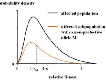
Multifactorial threshold model. We assume the multifac-torial threshold model [1], in which quantitative traits such as liability to the disease are determined by multiple genetic and non-genetic factors including a stochastic and/or an epinon-genetic effect. Under this assumption, the relative fitness as a quantitative trait in the affected population is determined by multiple factors and approximately follows a gamma distribution with a mean 1{s (Figure 2). (sis the selection coefficient of SZ; the mean relative fitness in the normal population is defined as unity.)

Table 12.Epidemiological data by Haukka et al. [17].

N S P Total (S+P)/Total

#of females 410,093 11,873 4,784 426,750 0.03903

#of female children 366,460 10,969 1,917 379,346 0.03397

{D~0:00506|ð1{rÞv5:06|10{3

(10)

The distribution curve of the fitness in the affected subpopu-lation with an allele Mnever shifts to the right unless M has a strong protective effect (i.e. an effect of elevating the affected carrier’s fitness by reducing the severity of the disease). Since a pathogenic allele for a deleterious disease can be assumed not to elevate the affected carrier’s fitness, the relative fitness in the affected subpopulation with the susceptibility allele M approxi-mately follows a gamma distribution with a mean not greater than

1{_s(i.e.1{_s_M;sƒ_s_Mv1).

No special assumptions else are required on the allelic structure in each locus, penetrance of each susceptibility gene, and possible interactions among the loci. It should be noted that the nuclear single major gene locus model is included as a special case in the assumptions.

2. Notation

Risk loci, two equivalent classes of alleles, and allele frequencies. Suppose that there arenrisk lociL1,L2,:::,LNfor SZ and that each locus has two equivalent classes of alleles: pathogenic and non-pathogenic. Let PP~i~fPikg and NN~i~ Nij

denote these classes at the risk locusLi. When subscriptsiand k are omissible, we simply use the symbolsL,M, andMM~ to denote a risk locus, a pathogenic allele at the risk locus, and the pathogenic class of alleles includingMat the locus, respectively.

Letj jMA,j jMU, andj jMGdenote the frequency of an alleleM in the affected, the unaffected and the general population, respectively. We define PP~i

A, PP~i

U, and PP~i

Gby the equations:

~ P Pi _A~ P

kjPikjA, PP~i

_U~

P

kjPikjU, and PP~i

_G~

P

kjPikjG. From definition we have the following equations: for a given pathogenic alleleM,j jMG~p Mj jAzð1{pÞj jMU, or

M

j jA{j jMG~ð1{pÞ j jMA{j jMU

: ð1Þ

Cross-generational reductions of the population fre-quencies of the pathogenic alleles due to the decreased

reproductive fitness of the affected population. {D_M_M~

_G~

cross-generational reduction ofMM~

_Gby natural selection {D_{j j}_M

G~ cross-generational reduction of j jMG by natural selection

It may be trivial that{D_P_P~_i

G~ P

k{DjPikjG§{DjPikjG.

Therefore we have: {D_M_M~

_G§{Dj jM_G: ð2Þ

Mutation and mutation rates. Mutation occurs in the following directions at each risk locus Li: ~NNi?PP~i, NN~i?NN~i,

~

P

Pi?PP~i, orPP~i?NN~i. Therefore, we use the following notations: mð Þi~ mutation rate at the risk locus Li, mð Þi N?P~ rate of mutation which occurs in the direction NN~i?PP~i at the locus Li, mð Þi_N

?N~rate of mutation which occurs in the directionNN~i?NN~i at the locusLi, mð ÞiP?P~rate of mutation which occurs in the directionPP~i?PP~iat the locusLi,mð ÞiP?N~rate of mutation which occurs in the direction PP~i?NN~i at the locus Li, mð Þi p~ rate of mutation which produces pathogenic alleles at the locusLi,m~ mutation rate at the risk locusL, m_M~ rate of mutation which produces the pathogenic allele Mat the locus L, m_M_M~~ rate of mutation which produces the pathogenic alleles at the locusL.

From definition we have:mð Þi~mð Þi _N ?Pzm

i

ð Þ_N

?Nzm i

ð Þ_P

?Pz mð Þi

P?N,mð Þi P~mð Þi N?Pzm(i)P?P{m(i)P?Nvm(i), andmð Þi Pikƒ mð Þi_Pvmð Þi_.

Therefore we have: m_Mvm_M_M~vm: ð3Þ

Mutation2selection balance ineach risk locus implies :

{D_M_M~

_G~m_M_M~: ð4Þ

3. Deduction of the persistence criteria

Now we proceed to deduce the persistence criteria. From the assumptions it follows that j jM 0_G_{, the population frequency of}

the pathogenic allele M in the next generation, is given by:

M

j j0_G~p Mj jA

:ð₁{sMÞzð1{pÞ:j jMU:1

p:ð1{sÞzð1{pÞ:1 ~

M

j jG{sMp Mj jA

1{sp ƒ

M

j jG{sp Mj jA

1{sp .

Therefore the reduction of the population

frequency of the allele M per generation is: {D_{j j}_M

G~

M

j jG{j jM 0G§j jMG{

M

j jG{sp Mj jA

1{sp ~

sp Mj jA{j jMG

1{sp ~

spð1{pÞ j jMA{j jMU

1{sp From (2), (3) and (4) it follows: spð1{pÞ j jMA{j jMU

1{sp ƒ{Dj jMGƒ{DMM~

_G~m_M_M~vm.

Thus we have the first criterion for a susceptibility gene (criterion A):

Criterion A. j jMA{j jMUvv, where n is defined by

v~ð1{spÞm

1{_p

ð Þsp.

Criterion A implies:j jMAvj jMUzv. Since the odds ratio (OR)

of the alleleM, defined byOR~j jMA 1 {_{j j}MU

1{_{j j}_M A

M j jU

, is monotonically

increasing for0vj jMAv1, it may be trivial: if0vj jMUv1{v,

OR~ j jMU zv

1{_{j j}M_U

1{ _{j j}MUzv

M j jU

~₁z v

M

j jU 1{v{j jMU

.

Thus we have the second criterion for a susceptibility gene (criterion B):

Criterion B. If0v_{j j}MUv1{v,ORv1z

v M

j jU 1{v{j jMU

.

Since criterion A also implies j jMA{vvj jMU and OR is monotonically decreasing for0vj jMUv1, we can easily see: if

1{vv_{j j}MUv1,OR~

M

j jA 1{j jMA{v

1{_{j j}MAzv

M

j jA{v

~1z

v

1{_{j j}MA

M

j jA{v

: Figure 2. Distribution of the relative fitness in the affected

population.In the multifactorial threshold model, the relative fitness as a quantitative trait in the affected population is assumed to approximately follow a gamma distribution with the mean1{s. The distribution curve in the affected subpopulation with an alleleM_shifts

to the right only ifM_{has a strong protective effect. Thus it can be}

assumed that the relative fitness in the affected subpopulation with a pathogenic alleleM_{approximately follows a gamma distribution with a}

(11)

It should be noted that ifv§1holds the persistence criteria are always fulfilled.

4. Numerical estimates of parameters in SZ genetics It is now known that mutation rates on autosomes and X chromosomes almost always fall within the range of 1026_{to 10}24 per locus per generation (usually v10{5_{; one generation = 20} years) [59,60]. Advancing parental ages could elevate the mutation rate [61]. Although it seems to increase as an exponential of the parental age in some loci, it can be approximated by a linear function of the parental age at least under 30 years for maternal age and under 40 years for paternal age [61]. On the other hand, large sampled cohort studies in Israel, Sweden and Denmark show that the mean age of parents in the general population is ,28 years for mothers and,31 years for fathers; the mean age of both parents is,29.6 years [62,63]. Therefore we can assume:

1:48|10{6_~29:6

20 |10

{6_v_m_v29:6

20 |10

4_~₁_:₄₈_|₁₀{4_:

We can know the values of the parameterspand s from the epidemiological studies. Among the many epidemiological studies on the fertility of SZ, the cohort study by Haukka et al. [17] is the largest in sample size (N = 870,093) and the lowest in sampling bias. They comprised all births in Finland during 1950–1959 and followed up through the National Hospital Discharge Register for Hospitalizations between 1969 and 1992. Estimated values forp and s are p~1:29|10{2 _and _s_~₆_:₅₄_|₁₀{1_{. Thus, we have:}

1:76|10{4_v_v_v₁_:₇₆_|₁₀{2_.

The estimated value ofvfor SZ may be remarkably small. This sums up the epidemiological characteristics of SZ which discriminate it from other common diseases with genetic bases such as type 2 diabetes and most adult cancers. For those diseases vwould be much greater due to much smaller svalues because most patients with those diseases manifest after the reproductive age (.40 years). On the other hand, SZ manifests typically in adolescence or early adulthood, and specific symptoms of the disease such as an autistic way of life and bizarre behaviors reduce the reproductive fitness of the patients as has been shown by most epidemiological studies.

It should be noted that contribution of advancing parental ages to pathogenic mutations seems not very large in SZ. That is because large sampled cohort studies have shown that the proportions of older parents both in the affected and the normal populations are equally small (,7.7% and,5.5% for fathers older than 45 years in the affected and the normal populations respectively; and,9.9% and ,8.7% for mothers older than 35 years) [64,65]. In addition, the differences in the mean ages of parents between the affected and the normal individuals are not very large (,1.7 years for fathers and ,0.8 year for mothers) [62,63] even if they are statistically significant.

Some researchers have proposed the hypothesis that SZ is associated with de novo mutations arising in paternal germ cells [62–66]. It is based on the observation (‘paternal age effect’) that the risk of SZ in the offspring seems to increase as paternal age advances from 20 years to over 50 years. However, the risk of SZ was also increased in the offspring of younger men (,21 years) [62,63,66] as well as in the offspring of younger women (,20 years) [63]. Therefore, major roles of paternally derived mutations in SZ seem to remain unsubstantiated. Indeed, no available data can exclude the possibility that the ‘paternal age effect’ on the risk of SZ may be due to putative maternal factors; while women in many countries today may be usually supposed to bear children

after the age of 20 years or to marry much older men only when the men have socio-economic benefits, predisposed women might bear children before the age of 20 years or choose too young or too old men as fathers of their children even if the men have no socio-economic benefits.

5. Validity-testing of the candidate genes in the literature with the criteria

We tested whether the 111 SNPs of the top 30 genes listed in the meta-analyses at SZGene (http://www.schizophreniaforum. org/res/szgene/default.asp) [30] meet the persistence criteria. Since SZGene is being periodically up-dated, we used the version on 10thAugust, 2009. Based on the genotype distribu-tions in meta-analyses, allele frequencies and the case-control differences were calculated. We also tested the top 100 SNPs listed in a recent GWAS by Need et al. [33] as well as the common variants reported in the latest GWASs by Shi et al. [31], by Stefasson et al. [34], and by The International Schizophrenia Consortium [32].

6. Power and sample size estimation in case-control association studies for SZ

Let W_:ð{?,?Þ_?ð0,1Þ be the cumulative distribution function of the standard normal curve and let W{1_:

0,1

ð Þ?ð{?,?Þ be its inverse function. The upper b point of the standard normal curve is given byzb~W{1ð1{bÞ and the

two sidedapoint byza~za=2. In a case-control association study of a single variantMwith sample size 2N(Ncases+Ncontrols) at a significance level a, the power 1{b is given by 1{b%

W

ffiffiffiffiffiffiffi 2N p

d{za

ffiffiffiffiffiffiffiffiffiffiffiffiffiffiffiffiffiffiffi 2xð1{xÞ

p

c

!

, or N%1

2

za

ffiffiffiffiffiffiffiffiffiffiffiffiffiffiffiffiffiffiffi 2xð1{xÞ

p

zzbc

d

!2

,

where x, c2_{, and} _d _{are defined by the equations:} _x_~

1

2 j jMAzj jMU

,c2_~_{j j}_M

A 1{j jMA

zj jMU 1{j jMU

, and

d~j jMA{j jMU. [67,68]

Since the criterion A (0vdvv) warrants0v1

2d

2_vv₂_x_ð₁_{_x_Þ

for 0.1,x,0.9, we have:c2_~₂_x_{1

2 ð Þ2x

2 zd2

n o

%2xð1{xÞ, or

c%pffiffiffiffiffiffiffiffiffiffiffiffiffiffiffiffiffiffiffi₂_xð₁{xÞ

. Thus we have:1{b%W ffiffiffiffiffiffiffi 2N

p

d{z a

ffiffiffiffiffiffiffiffiffiffiffiffiffiffiffiffiffiffiffi 2x(1{x) p c ! % W ffiffiffiffiffiffiffiffiffiffiffiffiffiffiffi N x(1{x) s

d{za

! vW

ffiffiffiffiffiffiffiffiffiffiffiffiffiffiffi

N x(1{x) s

v{za

!

, andN%zazzb

d

2

x(1{x)w

zazzb v

2

xð1{xÞfor 0.1,x,0.9.

We calculated the power of the association study for sample sizes N= 10000, 20000, 50000, 100000 under three levels of mutation rates. For the calculation ofNrequired in the association study for a single allele, we assume:a~0.05 and1{b~0.95, 0.8, 0.1. For the calculation of N required in GWAS, we assume: a~2:5|10{7_and₁_{_b_~_{0.95, 0.8, 0.1.}

Acknowledgments

We wish to thank Dr. Jun Ohashi (Tsukuba University, Ibaraki, Japan) for critical reading of the manuscript and valuable advice for revision. Especially, his advice was helpful in estimating the power and sample size of case-control association studies.

Author Contributions

(12)

References

1. Risch NJ (2000) Searching for genetic determinants in the new millennium. Nature 405: 847–856.

2. Tandon R, Keshavan MS, Nasrallah HA (2008) Schizophrenia, ‘‘just the facts’’ what we know in 2008. 2. Epidemiology and etiology. Schizophr Res 102: 1–18. 3. Jablensky AV (1995) Schizophrenia: the Epidemiological Horizon. In: Hirsch SR, Weinberger DR, eds. Schizophrenia. London: Blackwell Science. pp 206–252.

4. Harrison G, Cooper JE, Gancarczyk R (1991) Changes in the administrative incidence of schizophrenia. Br J Psychiatry 159: 811–816.

5. Osby U, Hammer N, Brandt L, Wicks S, Thinsz Z, et al. (2001) Time trends in first admissions for schizophrenia and paranoid psychosis in Stockholm County, Sweden. Schizophr Res 47: 247–254.

6. Essen-Mo¨ller E (1935) Untersuchungen u¨ber die Fruchtbarkeit gewisser Gruppen von Geisteskranken. Acta Psychiatr Neurol 8: 1–314.

7. Bo¨o¨k JA (1953) A genetic and neuropsychiatric investigation of a North-Swedish population. Acta Genet et Stat Med 4: 1–100.

8. Slater E, Hare H, Price J (1971) Marriage and fertility of psychiatric patients compared with national data. Soc Biol 18: S60–S73.

9. Larson CA, Nyman GE (1973) Differential fertility in schizophrenia. Acta Psychiatr Scand 49: 272–280.

10. Ødega˚rd Ø (1980) Fertility of psychiatric first admissions in Norway, 1936-1975. Acta Psychiatr Scand 62: 212–220.

11. Haverkamp F, Propping P, Hilger T (1982) Is there an increase of reproductive rates in schizophrenics? I. Critical review of the literature. Arch Psychiatr Nervenkr 323: 439–450.

12. Nanko S, Moridaira J (1993) Reproductive rates in schizophrenic outpatients. Acta Psychiatr Scand 87: 400–404.

13. Fananas L, Bertranpetit J (1995) Reproductive rates in families of schizophrenic patients in a case-control study. Acta Psychiatr Scand 91: 202–204. 14. Bassett AS, Bury A, Hodgkinson KA, Honer WG (1996) Reproductive fitness in

familial schizophrenia. Schizophr Res 21: 151–160.

15. Nimgaonkar VL (1998) Reduced fertility in schizophrenia: here to stay? Acta Psychiatr Scand 98: 348–353.

16. McGrath JJ, Hearle J, Jenner L, Plant K, Drummond A, et al. (1999) The fertility and fecundity of patients with psychoses. Acta Psychiatr Scand 99: 441–446.

17. Haukka J, Suvisaari J, Lonnqvist J (2003) Fertility of patients with schizophrenia, their siblings, and the general population: a cohort study from 1950 to 1959 in Finland. Am J Psychiatry 160: 460–463.

18. Crow TJ (1995) A Darwinian approach to the origin of psychosis. Brit J Psychiatry 167: 12–25.

19. Bru¨ne M (2004) Schizophrenia – an evolutionary enigma? Neurosci Biobehav Rev 28: 41–53.

20. Keller CK, Miller G (2006) Resolving the paradox of common, harmful, heritable mental disorders: Which evolutionary genetic models work best? Behav Brain Sci 29: 385–452.

21. Huxley J, Mayr E, Osmond H, Hoffer A (1964) Schizophrenia as a genetic morphism. Nature 204: 220–221.

22. Karlsson JL (1974) Inheritance of schizophrenia. Acta Psychiatr Scand 247 (Suppl): 77–88.

23. Kinney DK, Richards R, Lowing PA, LeBranc D, Zimbalist ME, et al. (2001) Creativity in offspring of schizophrenic and control parents: an adoption study. Creativity Research Journal 13: 17–25.

24. Shaner A, Miller G, Mintz J (2004) Schizophrenia as one extreme of a sexually selected fitness indicator. Schizophr Res 70: 101–109.

25. Lindelius R (1970) A study of schizophrenia. A clinical, prognostic and family investigation. Acta Psychiatr Scand Suppl 216.

26. Buck C, Hobbs GE, Simpson H, Winokur JM (1975) Fertility of the sibs of schizophrenic patients. Brit J Psychiatry 127: 235–239.

27. Rimmer J, Jacobsen B (1976) Differential fertility of adopted schizophrenics and their half-siblings. Acta Psychiatr Scand 54: 161–166.

28. Erlenmeyer-Kimling L (1978) Fertility of psychotics: demography. In: Cancro R, ed. Annual Review of the Schizophrenic Syndrome. New York: Brunner/Mazel 5: 298–333.

29. Svensson AC, Lichtenstein P, Sandin S, Hultman CM (2007) Fertility of first-degree relatives of patients with schizophrenia: A three generation perspective. Schizophr res 91: 238–245.

30. Allen NC, Bagades S, McQueen MB, Ioannidis JPA, Kavvoura FK, et al. (2008) Systematic Meta-Analyses and Field Synopsis of Genetic Association Studies in Schizophrenia: The SZGene Database. Nat Genet 40: 827–834.

31. Shi J, Levinson DF, Duan J, Sanders AR, Zheng Y, et al. (2009) Common variants on 6p.22.1 are associated with schizophrenia. Nature (Published online 1 July 2009;doi:10.1038/nature08192).

32. The International Schizophrenia Consortium (2009) Common polygenic variation contributes to risk of schizophrenia and bipolar disorder. Nature (Published online 1 July 2009;doi:10.1038/nature08185).

33. Need AC, Ge D, Weale ME, Maia J, Feng S, et al. (2009) A Genome-Wide Investigation of SNPs and CNVs in Schizophrenia. PLoS Genet 5(2): e1000373. doi:10.1371/journal.pgen.1000373.

34. Stefasson H, Ophoff RA, Steinberg S, Andreassen OA, Cichon S, et al. (2009) Common variants conferring risk of schizophrenia. Nature (Published online 1 July 2009;doi:10.1038/nature08186).

35. Lander ES (1996) The new genomics: global view of biology. Science 274: 536–539.

36. Reich DE, Lander ES (2001) On the allelic spectrum of human disease. Trends Genet 17: 502–510.

37. Pritchard JK (2001) Are rare variants responsible for susceptibility to complex diseases? Am J Hum Genet 69: 124–137.

38. Pritchard JK, Cox NJ (2002) The allelic architecture of human disease genes: common disease-common variant … or not? Hum Mol Genet 11: 2417–2433. 39. Mah S, Nelson MR, DeLisi LE, Reneland RH, Markward N, et al. (2006) identification of the semaphoring receptor PLXMA2 as a candidate for susceptibility to schizophrenia. Mol Psychiatry 11: 471–478.

40. Lenz T, Morgan TV, Athanasiou M, Dain B, Reed CR, et al. (2007) Converging evidence for a pseudoautosomal cytokine receptor gene locus in schizophrenia. Mol Psychiatry 12: 572–580.

41. Kirov G, Zaharieva I, Georgieva L, Moskvina V, Nikolov I, et al. (2008) A genome-wide association study in 574 schizophrenia trios using DNA pooling. Mol Psychiatry (doi10.1038/mp.2008.33).

42. Shifman S, Johannesson M, Bronstein M, Chen SX, Collier DA, et al. (2008) Genome-wide association identifies a common variant in the reelin gene that increases the risk of schizophrenia only in women. PLoS Genet 4(2): e28. doi:10.1371/journal.pgen.0040028.

43. O’Donovan MC, Craddock N, Norton N, Williams H, Peirce T, et al. (2008) Identification of loci associated with schizophrenia by genome-wide association and follow up. Nat Genet.

44. Sullivan PF, Lin D, Tzeng JY, van den Oord E, Perkin D, et al. (2008) Genomewide association study for schizophrenia in the CATIE study: results of stage I. Mol Psychiatry 13: 570–584.

45. Sanders AR, Duan J, Levinson DF, Shi J, He D, et al. (2008) No significant association of 14 candidate genes with schizophrenia in a large European ancestry sample: implication for psychiatric genetics. Am J Psychiatry 165: 497–506.

46. Friedman JI, Vrijenhoek T, Markx S, Janssen IM, van der Vliet WA, et al. (2008)CNTNAP2gene dosage variation is associated with schizophrenia and epilepsy. Mol Psychiatry 13: 261–266.

47. Kirov G, Gumus D, Chen W, Norton N, Georgieva L, et al. (2008) Comparative genome hybridization suggests a role forNRXN1andAPBA2in schizophrenia. Hum Mol Genet 17: 458–465.

48. Stefasson H, Rujescu D, Cichon S, Pietila¨inen OP, Ingason A, et al. (2008) Large recurrent microdeletions associated with schizophrenia. Nature 455: 232–236.

49. The International Schizophrenia Consortium (2008) Rare chromosomal deletions and duplications increase risk of schizophrenia. Nature 455: 237–241. 50. Walsh T, McClean JM, McCarthy SE, Addington AM, Pierce SB, et al. (2008) Rare structural variants disrupt multiple genes in neurodevelopmental pathways in schizophrenia. Science 320: 539–543.

51. Xu B, Roos JL, Levy S, van Rensburg EJ, Gogos JA, et al. (2008) Strong association of de novo copy number mutations with sporadic schizophrenia. Nat Genet 40: 880–885.

52. Repping S, van Daalen SKM, Brown LG, Korver CM, Lange J, et al. (2006) High mutation rates have driven extensive structural polymorphism among human Y chromosomes. Nat Genet 38: 463–467.

53. Sigurd–

ardo´ttir S, Helgason A, Gulcher JR, Stefansson K, Donnely P (2000) The mutation rate in the human mtDNA control region. Am J Hum Genet 66: 1599–1609.

54. Doi N, Hoshi Y (2007) Persistence problem in schizophrenia and mitochondrial DNA. Am J Med Genet Part B 144: 1–5.

55. Doi N, Itokawa M, Hoshi Y, Arai M, Furukawa A, et al. (2007) A resistance gene in disguise for schizophrenia? Am J Med Genet Part B 144: 165–173. 56. Marchbanks RM, Ryan M, Day IN, Owen M, McGuffin P, et al. (2003) A

mitochondrial DNA sequence variant associated with schizophrenia and oxidative stress. Schizophr Res 65: 33–38.

57. Munakata K, Iwamoto K, Bundo M, Kato T (2005) Mitochondrial DNA 3243A.G mutation and increased expression ofLARS2gene in the brains of patients with bipolar disorder and schizophrenia. Biol Psychiatry 57: 525–532. 58. Martorell L, Segue´s T, Folch G, Valero J, Joven J, et al. (2006) New variants in

the mitochondrial genomes of schizophrenic patients. Eur J Hum Genet 14: 520–528.

59. Vogel F, Motulsky AG (1997) Human genetics: problems and approaches. Berlin: Springer-Verlag.

60. Nachman MW, Crowell SL (2000) Estimate of the mutation rate per nucleotide in humans. Genetics 156: 297–304.

61. Risch N, Reich EW, Wishnick MM, McCarthy JG (1987) Spontaneous mutation and parental age in humans. Am J Hum Genet 41: 218–248.

62. Malaspina D, Harlap S, Fennig S, Heiman D, Nahon D, et al. (2001) Advancing paternal age and the risk of schizophrenia. Arch Gen Psychiatry 58: 361–367. 63. El-Saadi O, Pedersen CB, McNeil TF, Saha S, Welham J, et al. (2004) Paternal

and maternal age as risk factors for psychosis: findings from Denmark, Sweden and Australia. Schizophr Res 67: 227–236.

64. Zammit S, Allebeck P, Dalman C, Lundberg I, Hemmingson T, et al. (2003) Paternal age and risk for schizophrenia. Brit J Psychiatry 183: 405–408. 65. Byrne M, Agerbo E, Ewald H, Eaton WW, Mortensen PB (2003) Parental age

(13)

66. Sipos A, Rasmussen F, Harrison G, Tynelius P, Lewis G, et al. (2004) Paternal age and schizophrenia; a population based cohort study. BMJ;doi:10.1136/ bmj.38243.672396.55 (published 22 October 2004).

67. Ohashi J, Yamamoto S, Tsuchiya N, Hatta Y, Komata T, et al. (2001) Comparison of statistical power between 26_{2 allele frequency and allele}

positivity tables in case-control studies of complex disease genes. Ann Hum Genet 65: 197–206.