The reasons behind the progression in PISA scores: An education production function approach using semi-parametric techniques

A Thesis, presented as part of the requirements for the Award of a Research Masters

Degree in Economics from the NOVA

–

School of Business and Economics.

The reasons behind the progression in PISA scores: An

education production function approach using

semi-parametric techniques

Pedro Freitas, Student number 38

A project carried out on the Research Masters in Economics, under the supervision of:

The reasons behind the progression in PISA scores: An

education production function approach using

semi-parametric techniques

Pedro Freitas †

Nova School of Business and Economics, Universidade Nova de Lisboa

April 30, 2015

Abstract

On December 2013, and for the fifth time since 2000, OECD published the results of the latest PISA survey, providing a view on how the students’ performance has progressed during the last 12 years. Using PISA data we follow an education production function, which states that variables related to students, their family and the school explain the output, measured as the individual student achievement. Exploring the concept of efficiency we measure the ability that each student has to transform the given inputs into higher academic outcomes. Such analysis was performed through the estimation of an efficient frontier,derived by non-parametric techniques, namely Data Envelopment Analysis (DEA). Using this methodology we establish two vectors of analysis. The first one intends to disentangle the reasons behind the evolution in PISA scores across the years, concluding that the variation in inputs is on the core of the reasons to explain the evolution in PISA results. The second aims to evaluate what are the sources of student’s efficiency. On this topic we particularly explore the role of the school inputs, concluding that students with a more favourable socio-economic background are more indifferent to variables such as class size and school size.

JEL classification: I21,C61,C67.

Keywords:Education production function; Efficiency; Data envelopment analysis; PISA.

∗

I am greatly indebted to my supervisor, Ana Balc˜ao Reis, for the unexcelled guidance and encouragement and whose advice enormously improved this work. I acknowledge the computational help given by Lu´ıs Catela Nunes. I thank as well Jos´e Manuel Cordero-Ferrera for the help with Matlab coding. I appreciate the comments from the participants in the research group of Nova SBE, in the XXIII Meeting of the Economics of Education Association, Valencia 2014 and in the Third Lisbon Research Workshop on Economics, Statistics and Econometrics of Education. A reference as well to the support and comments from my Research Master and Phd colleagues namely, Marta Lopes, Jo˜ao Santos, Marta Rocha, Catarina ˆAngelo, Sofia Oliveira and Maria Ana Matias. Finally a very special acknowledgment to Jo˜ao Vaz, whose friendship, support and wisdom were so important during all this time and who shows in every moment the truth in Beckett’s sentence: ”Friendship, according to Proust, is the negation of that irremediable solitude to which every human being is condemned.”

†

1

Introduction

PISA is a set of three tests in the fields of reading, mathematics and sciences targeting students between 15 and 16 years old and organized every three years by OECD since 2000. Taking advantage of the availability of data covering a period of 12 years we intend to address two issues; identify the drivers behind the evolution in PISA scores and assess the reasons that justify the students’ relative level of efficiency. In our specific case we have used data from Portugal, which has been a participating country in PISA since 2000, showing a consistent, but not constant evolution during this time period.1

Regarding the motives behind the evolution in PISA scores, previous work tried to iden-tify them, particularly Pereira (2011) for Portugal and Osorioet al. for Indonesia (2011). Both papers followed an Oaxaca-Blinder decomposition, which consists in explaining the change in PISA scores through linear regressions and observe if this is attributed to the explanatory variables or to the evolution in the regression coefficients.2

Instead of following this decomposition approach we opted for a frontier analysis, which adds an efficiency perspective to the education production function, deriving relative measures across the students. Under such analysis, we propose that students combine a set of variables related to them, to their families and to their school (e.g. the inputs) in order to obtain a certain level of academic achievement (e.g. the output). The ones who use these variables in the most efficient way, define what is named as the efficient frontier, and all the remaining students are considered as inefficient.Thus this method-ology enables us to define a standard for comparing different students conditioning on their specific characteristics and their academic results.

To construct the efficient frontier two paths can be followed: 1. A parametric estimation, following a stochastic frontier analysis; 2. A non-parametric approach, namely through the use of Data Envelopment Analysis (DEA). Examples of the first approach can be found in the literature in works such as Pereira and Moreira (2011), which studies the efficiency of the Portuguese secondary schools, Perelman and Sant´ın (2005), on the ef-ficiency of the Spanish students using PISA data or Ryan (2013) who uses a stochastic frontier analysis to indentify the reasons for the decline in Australian PISA scores. Given the puzzling results often obtained from standard parametric estimations, the use of non-parametric approaches has gained attention in the literature, as referred by Worthington (2001), who points out two main reasons for the attractiveness of these methodologies. By one side it is mentioned the freedom in the relation between inputs

1_{A graphical summary of the evolution of the Portuguese performance in PISA can be seen in}

AppendixA₁. AppendixA₂presents a brief view on the structure of the Portuguese education system.

2_{Pereira (2011) concluded that from 2003 to 2006 the evolution in the variables level was the dominant}

and outputs, particularly in education contexts where some of the usual axioms of pro-ductivity may breakdown (e.g. cost minimization). It is referred as well that many times in standard statistical approaches the desired set of data is not available, which makes approaches that impose few restrictions on data, such as DEA, more attractive.

Thus, we propose a DEA model previously used in economics of education literature, but contrasting to previous applications of this methodology we have enlarged the analysis in three particular ways: 1. We have followed a regression based election of inputs, in order to reduce the level of ad-hoc choice of the inputs to be included in the frontier estimation, 2. We have used data from several periods and compared the results across time; 3. Since we aim to center the analysis at the student level, we are able to derive an efficiency score for each one of the students who participated in PISA since 2003, allowing us to identify the position of each student in relation to the efficient frontier. More than simply stating what are the reasons behind the evolution in PISA scores we aim to use the frontier approach to explain the sources of the students’ efficiency. To this propose we have divided the analysis into two main parts: the first explains what are the socio-economic environmental factors behind the relative efficiency of each stu-dent, namely the wealth of family or the parents’ schooling level. Secondly we evaluate in which way the allocation of school resources contribute to the students’ efficiency, namely who are the students that have been able to take more advantage of the school resources available. In the context of school inputs we also purpose an approach, based on Data Envelopment Analysis techniques, to assess how a different allocation of school resources, in particular school size and class size, may change or not the students’ achievement. Section 2 provides a theoretical framework to the question studied; section 3 presents the PISA data used; sections 4 describes the methodology and the results on the reasons behind the evolution in PISA scores, section 5 presents the factors that determine the students’ efficiency and finally section 6 concludes.

2

Theoretical background

old) leading us to follow what Todd and Wolpin call a contemporaneous model, where the variables used to explain the output (the student’s academic performance) should be able to capture the past history of inputs. Considering a certain student, i, which lives in household, j, and studies in school,s, we assume:

Tijs=T(Stijs;Fijs;Sijs) +ǫijs (1)

WhereTijs is the student’s achievement, measured by the score in a particular test, and

it is a function of: 1. Student’s characteristics, St_ijs; 2. Family inputs,F_ijs; 3. School inputs, Sijs; 4. An additive error, which includes all the unobserved characteristics of

the individual,ǫijs.

Building on this specification we propose a similar framework, to which we add a pro-ductivity factor, Aijs, standing for the ability students have to use the set of inputs

available to generate their output:

Tijs =T(Aijs, Stijs;Fijs;Sijs) (2)

We combine this concept of education production function with the notion of efficiency. Koopmans (1959) defined technical efficiency as the capacity to maximize the output conditional on the level of the inputs. The agents who can achieve such maximization are the ones who define the efficient frontier, and as Farrell (1957) referred inefficiency is determined as deviations from this same frontier. Thus, the set of efficient points, or in our case efficient students, are the ones who are on the frontier and the inefficient are the ones who are below the frontier.

Using this approach we have derived the education production frontier, and use it to study the three possible reasons to explain the evolution in PISA results: 1. An overall improvement in efficiency, meaning that more students are closer to the frontier; 2. A shift in the education frontier (e.g. the students’ ability to transform inputs in outputs); 3. The inputs related to the student, his family and the school increased.3

These three hypotheses are tested, concluding on which ones seem more plausible to ex-plain the Portuguese case.4 Among the three reasons presented, the first two correspond to a shock in the term, (Aijs), considering the specification in (2).5

3

Data

We have used the PISA dataset, which has the virtue of having a rich set of variables gathered though several questionnaires designed by OECD. There are 5 PISA surveys available from 2000 to 2012, although the initial year was excluded from our analysis due to the difference between the number of individuals who performed the reading and mathematics test, remaining so with 4 PISA samples (2003, 2006, 2009 and 2012). The survey intends to be a representative sample of the 15 years old student population at the time it is performed. To preserve this representativeness criteria, PISA dataset includes weights for each observation which, as recommended by OECD, are taken in consideration in all our steps to support the results.6

In order to meet the theoretical formulation presented in equations (1) and (2), the variables chosen for the analysis were grouped in factors attributed to the student, the student’s family and the school. Since we are working with data from several years, the choice of variables was subject to the existence and comparability across several PISA surveys. For example two variables that could be taken as school inputs, the index Respres (which stands for the level of autonomy in resources management) or the per-centage of repeaters at the school had to be dropped from the analysis, the first because its scale of measurement changed from 2003 to 2006 and the latter due the fact that such question was not included in the schools questionnaires in 2012.

When treating the data we took advantage of the indexes released by PISA, which aggre-gate several answers given by students and schools in the questionnaires.7 _{These indexes}

reveal to be important to define proxies, for example for students’ family economic situa-tion, which is measured by the Index of Home Possessions (Homepos). PISA also release the family Index of Cultural Possessions (Cultpos) and Educational Resources at home

4_{A graphical illustration of these possibilities can be seen in Appendix A} 3.

5_{Translating these three hypothesis into the case of an Oaxaca-Blinder decomposition, the first two}

cases correspond to a change in the coefficient and the third case to a change in the variables level. Through the proposed approach it is possible to derive a more refined analysis that trough an Oaxaca-Blinder methodology, since the evolution in coefficients is divided into two possible sources.

6_{The methodology followed by OECD to construct and weight the sample can be found in PISA}

Data Analysis Manual and PISA Technical Reports.

7_{Todd and Wolpin (2003) advice against the use of proxies. However its use reveals to be necessary}

(Hedres). We have used these three indexes all together to measure the proportional in-vestment of the student’s family in cultural possessions and educational resources given by the variables, Cultposinv and Hedresinv respectively:

Cultposinv= Cultpos

Homepos (3)

Hedresinv= Hedres

Homepos (4)

Attention was also given to existence of missing data. The percentage of missing data by variable is relatively low, but when combining several variables for empirical estimation, the sample can be significantly reduced (e.g. considering the variables chosen to the analysis, the samples are reduced for values between 50% in 2012 and 85% in 2009).8

In order to address this same problem, we have opted for the implementation of data imputation techniques, which can be divided in single and multi imputation. This last one was excluded since we need a single imputation for each missing observation, to apply the DEA method followed after. It was run an Expected Maximization algorithm9 to fill part of the missing data, making that the final imputed samples include at least 90% of the observations of the original sample.10

The variables which resulted from all the data treatment and the respective descriptive analysis can be observed in table below;

8_{Sample size without missing answers: 3462 (2003); 4014 (2006), 5535 (2009); 2831 (2012).} 9_{The explanation of this same algorithm can be found in appendix A}

4.

Table 3 .111

(weighted sample 2003-2012) PISA variable Interpretation Mean Sd Min Max

Student’s variables, Stijs

8th grade - 0.09 0.28 0 1

(dummy=1)

9th grade - 0.25 0.43 0 1

(dummy=1)

10th grade - 0.58 0.49 0 1

(dummy=1)

11th grade - 0.004 0.061 0 1

(dummy=1)

Academic Track Students enrolled in the standard academic track 0.87 0.34 0 1 (dummy=1)

Female

- 0.51 0.49 0 1

(dummy=1)

Age - 15.78 0.29 15 16.25

Family variables, Fijs

FISCED Father’s position in the international 2.52 2.03 0 6 standard classification of education, scale 0-6

MISCED Mother’s position in the international 2.49 2.04 0 6 standard classification of education, scale 0-6

Parents pt1 _{Students whose one of parents were born in Portugal}

0.12 0.33 0 1 (dummy=1)

Parents pt2 Students whose both parents were born in Portugal

0.83 0.37 0 1 (dummy=1)

CULTPOSinv Index of investment in cultural possessions at home 0.27 0.12 0.06 0.84 HEDRESinv Index of investment in educational resources 0.72 0.11 0.11 1.84 Homepos Index for level of home possession at home 7.2 0.98 0.58 11.21

School variables, Sijs

Non gov(%) Percentage of non-governmental financing of the school 16.75 22.5 0 100 Schools in small towns

- 0.31 0.46 0 1

(dummy=1) Schools in towns

- 0.4 0.49 0 1

(dummy=1) Schools in cities

- 0.16 0.36 0 1

(dummy=1) Schools in large cities

- 0.05 0.22 0 1

(dummy=1)

Percentage of girls in schools - 50.46 5.24 0.6 100

School size - 978.31 474.14 73 2750

Students/teacher ratio - 9.33 4.08 0.885 68 Scmatedu Index for level of quality of school resources 2.89 0.87 0.26 5.2 Class size12

- 22.52 4.66 1 53

Proportion of certified teachers - 89.01 18.46 0.6 100

Tschort Index for teacher shortage 1.26 0.6 0.79 5.59

N Number of students 20219 - -

-Nw Weighted Number of students 353,443 - -

-11_{Mean and standard deviations calculated based on the imputed sample.}

12_{For 2006 it corresponds to the average class size per school; and for the other years to the number}

Regarding the results obtained by the students in the PISA tests from the three subjects evaluated we focused our attention in the reading and mathematics ones13, denoting a negative evolution in the results from 2003 to 2006 and then a continuous progression between 2006 and 2012, that is more pronounced between 2006 and 2009:

Table 3.214

(weighted sample) 2003 ∆ 2006 ∆ 2009 ∆ 2012 Reading 481.05 -4.76 476.29 15.63 491.92 2.29 494.21

Mathematics 469.8 -0.44 469.36 20.03 489.39 4.25 493.64

4

Methodology and Results

The construction of the efficient frontier is performed through Data Envelopment Anal-ysis, whose non-parametric procedure has its roots in the paper by Charnes, Cooper and Rhodes (1978). The intensive use of DEA approaches to measure efficiency in education is found in works such as the ones by Kirjavainen and Loikkanen (1998) on the efficiency of the Finnish secondary schools, Portela (2011, 2012) on the efficiency of Portuguese secondary schools or Afonso and St Aubyn (2005) on cross country efficiency of sec-ondary education.

The wide majority of the literature applying DEA to education focus on the measure-ment of school efficiency, taking each school as a Decision Making Unit (DMU) (e.g. the entity responsible for converting inputs into outputs). We want to measure how each individual takes advantage of the available inputs, centring our analysis at the student level. This approach has several advantages, since it allows for an efficiency measurement for each individual student, constructing a DEA model with a significantly larger sample than the ones normally used. This path of study is much less usual in the literature, with few exceptions such as Waldo (2005), who applies DEA techniques to student individual data from the Swedish upper secondary schools.

For efficiency calculation it was pursued a DEA output oriented model with variable returns to scale based on the following linear programming problem:

13_{We have decided not to focus in Sciences since Reading and Mathematics are the two fields which}

are subject to national exams at the end of 9th grade, when students are around 14/15 years old.

14_{These scores do not necessarily match the ones officially reported by PISA, since even after the}

maxθ0

s.to:

θ0y0≤

n X

i=1

yiλi

x0 ≥

n X

i=1

xiλi

n X

i=1

λi = 1

λi ≥0

(5)

The problem presented above is solved for i+1 DMU’s, having each one the outputs y0

and the inputs x₀. This formulation stands for an output oriented model, where effi-ciency is read as the maximum amount of output that each DMU is able to generate with the inputs given. An efficient DMU is the one who is on the frontier which happens when θ₀ = 1, being it the minimum possile value of θ₀. All the efficiency scores higher than one correspond to inefficient units, and the higher the value ofθ0, the less efficient

is the respective DMU.15 The attractiveness of the DEA approach is that each unit is seen as a linear combination of the most efficient units closest to it, and the weight given to each one of this efficient units is given by the term λi. This way the performance of

each student is evaluated in relation to his peers. The assumption that the sum of all

λi equals one imposes variable returns to scale to our problem, as widely used in the

literature.16 Translating the general DEA framework to the specific case of our data, it is assumed a multiple output for each DMU, given by the score achieved in the reading and mathematics test.17_{Regarding the inputs choice we have chosen a methodology that}

decreased the level of discretion in its election. In DEA original formulations no particu-lar methods were advanced to determine what inputs may or may not be relevant in the construction of the production frontier.18_{In line with what was previously presented in}

Manceb´on-Torrubia et al. (2010) we have adopted a regression based methodology for the inputs choice, where estimation analysis were performed using PISA data and follow-ing the general theoretical formulation presented in equation (1). OLS regressions were

15_{For example if the value ofθ}

0 for a certain DMU equals 1.2, it means that with the same inputs,

that student could achieve a 20% higher output.

16_{A graphical representation of the frontier possibility set can be seen in Appendix 5.}

17_{These scores correspond to the average of the 5 plausible values released by PISA in both fields,}

Reading and Mathematics.

18_{Later literature on the topic of inputs choice in DEA can be found in works such as Nataraja and}

computed (as presented in equation 6) taking in consideration the 5 Plausible values and the population weights provided by PISA. The variance of the estimators was estimated by the Balanced Repeated Replication using the 80 population weights provided in the datasets and a Fay’s adjustment of 0.5, as recommended by PISA.19 The estimation was run separately for the reading and mathematics scores considering different cases: 1. Just the students without missing answers (2003-2012); 2. The imputed databases without control for year adjustments (2003-2012); 3. The imputed databases controlled for year dummies (2003-2012).

Tijs=β0+β1Stijs+β2Fijs+β3Sijs+ǫijs (6)

Additionally, and using the imputed sample controlled for year effects, it was performed an estimation following an Hierarchical Linear Model (HLM). The use of multilevel models has been growing in the economics of education literature, in works such as Manceb´on-Torrubia et al. (2010), Bowers and Urick (2011) or Agasisti and Cordero-Ferrera (2013). The PISA own publication already mentioned the possibility of using the PISA sample as a way to perform multilevel analysis.20 Assessing student performance is one of the examples that best fits the intention of an HLM, which controls for the fact that the observations are organized in several hierarchical structures (e.g each student is nested in a certain class, which is nested in a school, which belongs to a particular region). In our particular case we follow a two level model, being the first level the one correspondent to the student and the second one the one correspondent to the school. All slopes are fixed and only the intercept was randomized at the second level.21

Level 1-Model:

T_ijs=β_0s+β₁St_ijs+β₂F_ijs+ǫ_ijs (7)

19_{Further details on this methodology can be found in pages 79-85 of the PISA 2003 Data Analysis}

Manual.

20_{See Annex A8 ofPISA 2006: Science Competencies for Tomorrow’s World, Vol. 1.}

21_{For technical features underlying the estimation procedure of HLM see Woltman et al. (2012),}

Level 2-Model:

β_0s=γ₀+γ₁S_s+r_0s

β1=η1

β2=η2

(8)

The estimations using this HLM model correspond to the 4th case presented in the table below.

Table 4.1

5 plausible values reading/mathematics (2003-2012) Weighted sample

1 2 3 4

Reading Maths Reading Maths Reading Maths Reading Maths Student variables

Female 22.17*** -25.48*** 22.03*** -26.24*** 21.92*** -26.4*** 21.23*** -26.91***

(15.67) (-22.29) (16.92) (-24.71) (16.71) (-25.09) (17.81) (-24.27)

Age -22.83*** -22.63*** -22.14*** -22.04*** -18.92*** -17.24**** -16.63*** -15.79***

(-9.72) (-9.73) (-12.29) (-10.65) (-11.07) (-8.94) (-9.09) -8.02

8th 26.2*** 19.51*** 24.52*** (3.81) 26.82*** 19.05*** 26.67*** 19.81***

(4.4) (4.4) (5.9) 15.6*** (6.69) (4.97) (6.83) (5.55)

9th 74.92*** 69.86*** 74.37*** 67.44*** 75.36*** 68.92*** 73.83*** 69.04

(18.33) (3.81) (18.83) (19.19) (19.72) (21.28) (20.93) (23.67)

10th 144.32*** 142.30*** 143.78*** 139.97*** 145.22*** 142.09*** 140.75*** 141.84***

(33.07) (3.89) (36.01) (38.32) (37.32) (42.47) (41.56) (46.72)

11th 206.6*** 218.19*** 203.62*** 212.57*** 206.24*** 216.42*** 199.36*** 214.79***

(20.34) (21.54) (23.58) (23.7) (23.75) (24.00) (23.18) (24.04)

Academic track 21.04*** 18.6*** 21.39*** 19.42*** 22.94*** 21.71*** 26.78*** 23.56***

(7.35) (6.67) (8.48) (7.89) (8.91) (8.75) (10.18) (4.49)

Family variables

Mother - High school 5.48*** 7.00*** 5.14** 6.16*** 5.41*** 6.55** 4.34** 5.59***

(2.98) (3.86) (5.14) (3.65) (2.96) (3.78) (2.79) (3.52)

Mother -More than high school 3.16 8.36*** 5.72** 9.63*** 6.88*** 11.28*** 4.5*** 6.14***

(1.18) (3.06) (2.24) (3.87) (2.71) (4.59) (2.46) (3.63)

Father - High school 5.15*** 6.3*** 6.35*** 7.30*** 5.81*** 6.61*** 4.19* 8.7***

(2.67) (3.59) (4) (4.68) (3.66) (4.29) (1.89) (4.43)

Father -More than high school 6.87*** 10.67*** 7.40*** 11.54*** 6.85*** 10.89*** 6.22*** 10.79***

(2.86) (5.07) (3.65) (6.64) (3.44) (6.31) (2.48) (4.14)

Parentspt1 12.13*** 16.19*** 14.88*** 16.98*** 15.39*** 17.74*** 12.74*** 12.03***

(2.96) (3.54) (4.25) (4.21) (4.47) (4.54) 17.81 (3.69)

Parentspt2 8.8*** 13.44*** 11.49*** 14.29** 13.27*** 16.96*** 11.68*** 11.82***

(2.71) (3.199 (3.89) (3.69) (4.58) (4.49) 4.15 (3.79)

Cultpossinv 46.81*** 25.25*** 49.04*** 26.14*** 45.96*** 21.6*** 47.73*** 23.56**

(7.08) (4.48) (8.25) (4.96) (7.86) (4.13) (8.56) (4.49)

Hedresinv 2.3 -0.37 3.31 -1.25 13.77*** 11.23** 13.99** 14.09***

(0.44) (-0.06) (0.66) (-0.24) (2.45) (5.18) (2.74) (2.72)

Homepos 9.75*** 10.89*** 8.88*** 10.21*** 8.92*** 9.77*** 6.87*** 8.61***

School variables

% of non government financing 0.18*** 0.24*** 0.17*** 0.22*** 0.14*** 0.18*** 0.16*** 0.18***

(3.71) (4.3) (3.93) (4.74) (3.37) (4.09) (3.57) (4.43)

Small town 0.35 -4.02 0.31 -2.52 -0.17 -3.11 1.53 -3.16

(0.085) (-0.94) (0.83) (-0.66) (-0.05) (-0.79) 0.39 (-0.96)

Town 1.21 -4.26 0.58 -3.25 0.64 -3.12 3.37 -2.39

(0.27) (-0.89) (0.14) (-0.75) (0.16) (-0.73) (-0.67)

City 8.84* 4.38 13.11** 4.14 8.92** 4.6 12.24*** 5.93

(1.88) (0.92) (2.28) (0.92) (2.24) (0.98) (2.98) (1.44)

Large City 12.55** -1.35 13.11** -1.18 14.3** 0.65 18.24*** 2.18

(1.96) (-0.21) (2.28) (-0.19) (2.46) (0.11) (3.31) (0.41)

Percentage of girls 0.15 0.00 0.13 -0.05 0.32 0.24 0.34* 0.19

(0.63) (-0.024) (0.63) (-0.25) (1.63) (1.27) 1.68 (1.15)

Schoolsize 0.006* 0.0011 0.006** 0.002 0.005* 0.001 0.008** 0.0034

(1.93) (0.39) (2.04) (0.83) (1.94) (0.55) (2.68) (1.3)

Scmatedu 2.19* 2.68** 2.7** 3.09** 2.15* 2.29** 2.21 2.09**

(1.81) (2.06) (2.23) (2.52) (1.86) (2.25) (1.88) (2.01)

Stratio -0.21 -0.26 -0.18 -0.27 0.11 0.16 0.006 0.24

(-0.92) (-0.98) (-0.85) (-1.24) (0.39) (0.63) (1.02) (0.96)

Classize 0.32* 0.68*** 0.30* 0.69*** 0.29* 0.68*** -

-(1.65) (3.49) (1.69) (3.76) (1.67) (3.85) -

-Proportion of certified teachers 0.20*** 0.25*** 0.19*** 0.25*** 0.056 0.041 0.065 0.049

(2.99) (3.5) (3.31) (4.03) (1.00) (0.69) (1.082) (0.80)

TCSHORT -1.39 -2.27 -1.74 -2.25 -0.55 -0.49 -0.91 -1.11

(-0.75) (-1.43) (-1.06) (-1.62) (-0.36) (-0.42) (-0.625) (-0.88)

Constant 565.62*** 584.29*** 559.11*** 581.53*** 490.27*** 479.34*** 467.27*** 497.78***

(38.39 (38.39) (14.11) (18.24) (16.07) (15.95) (13.49) (16.2) (13.79)

Rsqr 0.49 0.48 0.49 0.48 0.49 0.49 -

-Year Dummies No No No No Yes Yes Yes Yes

Statistically significant at *10%. *5%. ***1%. T-ratios in parenthesis.

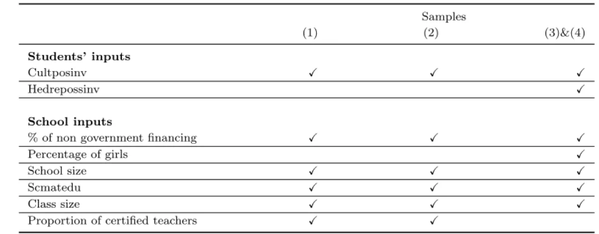
From the table above it is denoted some consistency across the different specifications presented but some differences when the reading or mathematics score are taken as the explained variable. We decided to include in the frontier estimation those that are significant at least at 10% level in one of the two test scores. For the frontier estimation we consider three different samples which reflect the input analysis performed above. The first two correspond to the completed sample and the imputed sample not controlled for year adjustments and the third one corresponds to the OLS (3) and HLM (4) analysis controlled for year dummies.

The inputs measurements must have non-zero elements, and when such cases occurs an infinitesimal value is assumed.22

The inputs were classified in two different categories. By one side we had to define those inputs that correspond to the environment where the student lives, and thus are not a choice of the student. In DEA literature these inputs are labelled as non-discretionary,

zi, and in our case correspond to: gender, age, mother’s and father’s level of education,

parents’ nationality, Index of Home possessions (Homepos) and geographic location. All the other inputs,xi, the discretionary, correspond to the ones that are indeed included

in DEA linear programming problem and that are presented in the table below. Later, in section 5, when we assess the sources of efficiency, the remaining inputs,zi, are then

included in the analysis.

Table 4.2

Samples

(1) (2) (3)&(4)

Students’ inputs

Cultposinv X X X

Hedrepossinv X

School inputs

% of non government financing X X X

Percentage of girls X

School size X X X

Scmatedu X X X

Class size X X X

Proportion of certified teachers X X

In what concerns the inputs, also to note that the variables regarding the grade and track of studies are essentially categorical variables, and they had to be disregarded from the DEA analysis. Thus it was estimated a pooled frontier, where all the students included in the PISA sample are considered. Although in order to incorporate in the analysis these important students’ characteristics, then efficient frontiers are derived grouping just those students who are enrolled in the same grade or track of studies. Through this approach we differentiate between a frontier where every student are compared across each other, to a case where students are compared with the ones who are in a similar academic position.

22_{Some of the indexes in the PISA dataset present negative values, since they are constructed in}

4.1 DEA efficiency scores - Results

Three different DEA were run for the samples (1), (2) and (3)&(4) considering as outputs the scores in reading and mathematics and as inputs the ones that result from the regression based choice performed above. Also to stress that the DEA results presented correspond to estimations in which all the students are included independently of the grade or track of studies they are enrolled in. In the following table is shown the quartile distribution on the efficiency scores, θ₀, derived:

Table 4.1.1

θ0 (weighted sample) 1st quartile Median 3rd quartile Mean

2003 1.16/1.17/1.15 1.27/1.28/1.27 1.41/1.43/1.41 1.31/1.33/1.31

2006 1.17/1.18/1.16 1.29/1.3/1.28 1.46/1.47/1.45 1.35/1.36/1.33

2009 1.18/1.18/1.15 1.29/1.29/1.27 1.44/1.45/1.42 1.33/1.33/1.31

2012 1.17/1.19/1.17 1.28/1.31/1.29 1.44/1.47/1.45 1.33/1.35/1.33

The three values presented for the efficiency scoreθ0correspond to the DEA estimation according to the

samples (1)/(2)/(3)&(4)

Observing the table above it is noticeable how the efficiency levels of the Portuguese students are rather constant across the years, particularly between 2006 and 2012. From all the four distributional points reported to emphasize how this constancy over time is particularly significant in the first quartile and the median, meaning that around the third quartile the efficiency levels seem to be more unstable during the time period considered. These conclusions are robust whether we consider the non-imputed or the imputed database.

Table 4.1.2

Meanθ0 (weighted sample) Private schools Public schools

2003 1.27/1.28/1.24 1.31/1.33/1.31

2006 1.3/1.29/1.27 1.36/1.36/1.34

2009 1.24/1.23/1.23 1.34/1.35/1.32

2012 1.24/1.25/1.22 1.34/1.37/1.34

The three values presented for the efficiency scoreθ0correspond to

DEA estimation according to the samples (1)/(2)/(3)&(4)

Table 4.1.3

Meanθ0 (weighted sample) 7th grade 8th grade 9th grade 10th grade 11th grade 2003 1.75/1.77/1.71 1.56/1.58/1.53 1.41/1.43/1.40 1.23/1.24/1.23 1.08/1.11/1.10

2006 1.79/1.81/1.76 1.52/1.53/1.49 1.37/1.37/1.35 1.23/1.24/1.22 1.16/1.16/1.15

2009 1.54/1.55/1.5 1.57/1.58/1.53 1.39/1.39/1.36 1.24/1.24/1.23 1.10/1.08/1.1

2012 1.62/1.65/1.61 1.5/1.56/1.54 1.37/1.4/1.38 1.25/1.26/1.24 1.11/1.14/1.09

When desegregating the results it is denoted that the stagnation of the efficiency seems to be happening across the private and public schools. When the levels of efficiency are disaggregated according to the students’ grade, we observe that in the grades correspon-dent to around 83% of the whole sample, 9th and 10th grade, there is a high stability of the efficiency scores across time. The other grades, namely the 7th show a higher level of instability since 2003.23 Additionally, it was observed that at the individual level, the correlation between the efficiency scores and the average scores in reading and mathematics is negative. Such fact means that higher the score in PISA test, the lower the value ofθ0, and then the more efficient is the individual.24

4.2 Malmquist Index - Comparing PISA across the years.

Caves, Christiansen and Diewert (1981) proposed the concept of Malmquist Index, al-lowing for efficiency evaluations of the same DMU across different points in time. This measure is particularly appealing for our analysis, since we are measuring efficiency in PISA considering several years. However, contrary to standard Malmquist Index appli-cations, the data used in this work is not panel data. PISA survey intends to be an accurate representation of the student population, and in each time different samples, with different sizes, of students between 15 and 16 years old are considered. This fact makes us use a modified version of the Malmquist Index presented by Camacho and Dyson (2006) [CDMI].25 In their formulation the authors intended to compare the effi-ciency performance across different groups. In our specific case, the samples of each of the years in analysis were considered as different groups and Malmquist indexes were computed for 2003-2006, 2006-2009 and 2009-2012. The Malmquist Index has also the interest of allowing to disaggregate between two possible sub-components: 1. Catch up component, standing for the measurement of the movement of the inefficient DMU’s to the frontier (efficiency change); 2. Frontiers shifts, namely measuring how from one pe-riod to the other the technology allows that with the same inputs higher level of outputs are obtained (technical efficiency).26

23_{To test for the possibility that the efficiency scores are being driven by top achieving students, the}

DEA’s for cases (2) and (3) were computed, considering just those students whose average score between reading and mathematics is below the 95th percentile for their grade. The results in AppendixA₆show that the inefficiency levels are lower, but the stability of the results remain as in the tables presented.

24_{A graphical representation of this same relation can be found in Appendix A} 7.

25_{CDMI, Camacho and Dyson Malmquist Index, following the nomenclature by Crespo-Cebada,}

Cha-parro and Sant´ın (2009).

26_{Note that originally, CDMI is used by Camacho and Dyson (2006) under constant returns to scale.}

CM I(x_t;y_t;x_t+1;y_t+1) =

(NQt

i=1

Dt(xt, yt))Nt1

(

NQt−1

j=1

Dt−1_(xt−1_{, y}t−1₎₎Nt1−1

.     

(NQt

i=1

Dt−1(xt, yt))Nt1

(NQt

i=1

Dt_(xt_{, y}t₎₎Nt1 .

(

NQt−1

j=1

Dt−1(xt−1, yt−1))

1

Nt−1

(

NQt−1

j=1

Dt_(xt−1_{, y}t−1₎₎Nt1−1

     1 2 (9)

D(x,y) stands for the distance function which can be read as the inverse of the efficiency score previous derived: θ0.27 The term outside the squares brackets represents the

efficiency change factor, measuring the efficiency gap between groups (in our particular case different PISA samples in different years)- catch up component. The expressions in brackets, represents the change in the frontier between different PISA samples (years)-frontier shift.28 Values equal to 1 stand for non progression in the different components of the CDMI, values lower than one stand for a negative evolution and higher than one for a positive one.

As it is observed in (9) the CDMI formulation is composed by ratios of different geometric means, which do not take into account the possibility that we are dealing with a weighted database, as it is the case of the PISA one. This fact leads us propose a modified version of the index named as Weighted Camacho and Dyson Malmquist Index (WCDMI), which differs from the one previously presented since it is composed of weighted geometric means:

W CM I(xt;yt;xt+1;yt+1) =

[

Nt Q

i=1

(Dt_(xt_{, y}t₎₎wi_]

1

NtP i=1wi

[

Nt−1

Q

j=1

(Dt−1_(xt−1_{, y}t−1₎₎wj_]

1

NtP−1

j=1 wj

.           [

N_Qt

i=1

(Dt−1_(xt_{, y}t₎₎wi_]

1

NtP i=1wi

[

N_Qt

i=1

(Dt_(xt_{, y}t₎₎wi_]

1

NtP i=1wi

. [ N_t −1 Q j=1

(Dt−1_(xt−1_{, y}t−1₎₎wj_]

1

NtP−1

j=1 wj

[

Nt−1

Q

j=1

(Dt_(xt−1_{, y}t−1₎₎wj_]

1

NtP−1

j=1 wj

          1 2 (10)

27_{In the same way that the higher the value of θ}

0 the lower the level of efficiency, for D(x,y) the

interpretation is reversed, meaning the lower the value of D(x,y), the higher the level of inefficiency. D(x,y) mainly corresponds to the output distance function proposed by Shepard (1970).

28_{The frontier shift component is a geometric mean of the cases when we take the technology in year}

From now one, given the coherence in the estimation results between the non-imputed and the imputed samples, just these last ones (2 and 3 4) are considered:

Table 4.2.129

(2)/(3)&(4)(weighted sample) Malmquist Index Catch-up Frontier Shift

2003-2006 ≈1.03/≈1.02 ≈0.96/≈0.97 ≈1.04/≈1.06

2006-2009 ≈1/≈1.04 ≈1/≈1 ≈0.99/≈1.04

2009-2012 ≈1.01/≈1.02 ≈0.98/≈0.98 ≈1.03/≈1.03

The two values presented for the Malmquist Index correspond to the samples (2)/(3)&(4)

The results showed on the Malmquist Index and in its two sub-components intend to infer on the first and second reasons presented in section 2 as possible drivers of the evolution in the Portuguese PISA results, which correspond to shocks in the productiv-ity factorAijs (equation 2). In order to assess if this possible technological shock really

explains the evolution in PISA scores, the analysis of the Malmquist Index should be put together with the own evolution in PISA scores depicted in table 3.2.

From 2003 to 2006 we observe contradictory movements between the two sub-components that constitute the Malmquist Index. If by one side the value lower than one for the catch-up factor indicates a deterioration in the global level of efficiency (e.g. on average the students are further way from the frontier), by the other side we witness a positive movement of the frontier shift, denoting a higher capacity of the students to transform inputs into outputs. Although to note that the size of this frontier shift effect seems to depend on the sample used, resulting that the total Malmquist Index show a value comprehended between 1.02 and 1.03. Recalling the evolution of the scores between these two same years, we observe a fall in the reading and mathematics results. The results provided by the Malmquist Index analysis do not show a total deterioration of efficiency, then the evolution in the productivity factorAij cannot be in the core of the

explanation for the evolution of the Portuguese PISA results.

Between 2006 and 2009 we observe that the catch-up factor remains rather constant in both cases (2 and 3&(4)). On the frontier shift side, and depending on the sample used, we observe that we may have a movement in the frontier, leading that the total Malmquist Index is lower bounded by a value of 1 and upper bounded by a value of 1.04. In this period we observe a significant increase in reading and mathematics PISA scores. The Malmquist Index is not able to give a definitive answer for this case, since the evidence on the size of productivity evolution depends on the case considered, and consequently it is not totally clear if it is enough to sustain the evolution in PISA scores. In the last period from 2009 to 2012, we note a slight deterioration in the catch-up com-ponent, compensated by a positive evolution in the frontier shift element. When they are aggregated, the Malmquist Index shows a small positive evolution in both cases.

29_{The same table but considering just those students whose average score between reading and}

Recalling that we observe a small progression in PISA scores in both subjects during these three years, it seems that the evolution in productivity fits the evolution observed in the PISA results.

Across the different Malmquist indexes we note that the frontier shift component has contributed to the improvement of the students’ efficiency, although the catch up factor has been having a negative contribution. These two facts put together provide evidence that the progression in efficiency has been driven by the positive evolution of the efficient students rather by the progression of the inefficient ones.

The results observed in the Malmquist Index are not conclusive for the evolution in PISA scores during the PISA waves that comprehend the period between 2003 and 2006 and show to be more insightful between 2006 and 2012. These conclusions make us explore the third possibility presented before, particularly if the evolution in the inputs levels may be a strong justification behind the evolution in the PISA results during this time span.

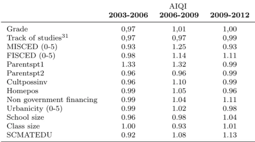
4.3 Inputs Change

To complement the results on the compared analysis between the results of the Malmquist Index and the results in PISA scores, we explore the increase in the inputs as the possible driver for the progression in PISA scores. To test for this possibility we have used what we named an Average Input Quantity Index (AIQI), which captures the change in the weighted mean of each input from one PISA survey to the other:

AIQI =

Nt

P

i=1

wiinputi

Nt

P

i=1

wi

Nt−1

P

j=1

wjinputj

Nt−1

P

j=1

wj

(11)

From all the inputs pointed at the begging of section 4, we have focused in those ones which proved to be strongly significant in all of the three regressions performed. The index is calculated for Nt students in year t and Nt−1 students in year t-1. wi and wj

Table 4.3.130

AIQI

2003-2006 2006-2009 2009-2012

Grade 0,97 1,01 1,00

Track of studies31 _{0,97 0,97 0,99}

MISCED (0-5) 0.93 1.25 0.93

FISCED (0-5) 0.98 1.14 1.11

Parentspt1 1.33 1.32 0.99

Parentspt2 0.96 0.96 0.99

Cultpossinv 0.96 1.10 0.99

Homepos 0.99 1.05 0.96

Non government financing 0.99 1.04 1.11

Urbanicity (0-5) 0.99 1.02 0.98

School size 0.96 0.98 1.04

Class size 1.00 0.93 1.01

SCMATEDU 0.92 1.08 1.13

In the table above, we can identify the evolution of thirteen inputs from 2003 to 2012. From 2003 to 2006 we can denote that out of the thirteen evaluated just one registered a positive evolution. The opposite movement is seen from 2006 to 2009 when nine of the inputs show values for the AIQI higher than one. Finally from 2009 to 2012 we see a mixed behaviour with five of the thirteen inputs studied increasing, four partially stag-nated (AIQI≈ 0.99) and the remaining ones decreasing. The evolutions just described must be compared with the evolutions of the PISA scores during the period considered, evaluating in which way the input variations match, or not, the PISA scores evolution. Recalling table 3.1 we observe that from 2003 to 2006 the PISA scores fell, which was followed by a large increase from 2006 to 2009 and to a more modest evolution from 2009 to 2012. The shape of this evolution seems to fit in the pattern of the input progression previously described.

Combining what was presented in sub-section 4.2 and 4.3, it is possible to summarize the conclusions on the reasons behind the evolution in the Portuguese PISA scores: 1. Between 2003 and 2006 despite the evolution in productivity, this has been contradicted by a general fall in the inputs level which lead to the deterioration of the PISA results; 2. Between 2006 and 2009 it may have happened a small technological shock in the ed-ucation production function which coincided with a general increase in the input levels, which appears as a strong reason to justify the significant progression in PISA scores; 3. From 2009 and 2012, we witness a positive evolution in the frontier shift factor, con-tradicted, in part, by a regression in the catch-up factor. We observe as well as mix behaviour of inputs, with ones increasing and others decreasing. These patterns show that all these effects put together contributed to the small progression registered in PISA results during this period.

30_{The table presents the results on the imputed sample.}

31_{Measured as the percentage of the curriculum that corresponds to the standard academic track,}

4.4 Enrolment grade and track of studies - Evidence from a separated frontier anal-ysis

In the analysis presented in sub-section 4.1, a unique frontier is constructed for each year, pooling every student in the sample, independently of their academic grade or track of studies. In this subsection we intend to take these two factors in consideration and divide the sample into different groups and run individual frontiers for each sub-group. Thus, we intend to construct frontiers in which each student is compared with the peers that are more alike with them in academic terms, and observe if the conclusions on the evolution of the Portuguese scores taken in the previous section remain. In the sample division according to students’ grade we have decided to consider two sub-groups: 1. The students in the lower secondary education, which corresponds to the ones that are enrolled between the 7th and 9th grade; 2. The students who are studying in the upper secondary education, which corresponds to the 10th and 11th grade. Considering the track of studies, two alternative divisions are performed: 1. The students who opted for a vocational track of studies; 2. The students who followed a standard academic school track. As before we initially report the distribution of efficiency scores for the different sub-groups from 2003 to 2012.

Table 4.4.1

θ0 (2)/(3) Lower secondary Upper secondary

weighted sample 1st Quartile Median 3rd Quartile Mean 1st Quartile Median 3rd Quartile Mean 2003 1,15/1,14 1,27/1,26 1,42/1,41 1,30/1,29 1,13/1,12 1,22/1,21 1,32/1,31 1,24/1,22 2006 1,19/1,16 1,32/1,30 1,48/1,45 1,36/1,33 1,13/1,11 1,22/1,21 1,31/1,31 1,23/1,22 2009 1,19/1,16 1,32/1,30 1,46/1,42 1,34/1,31 1,14/1,12 1,22/1,21 1,32/1,31 1,24/1,22 2012 1,24/1,23 1,39/1,37 1,56/1,53 1,42/1,40 1,15/1,12 1,24/1,22 1,35/1,32 1,25/1,23

The two values presented for the efficiency scoreθ0correspond to the DEA estimation according to the samples (2)/(3)&(4) Table 4.4.2

θ0 (2)/(3) Vocational track Academic track

weighted sample 1st Quartile Median 3rd Quartile Mean 1st Quartile Median 3rd Quartile Mean 2003 1,10/1,06 1,21/1,15 1,33/1,28 1,22/1,18 1,15/,15 1,27/1,26 1,41/1,40 1,31/1,30 2006 1,09/1,07 1,20/1,18 1,34/1,31 1,25/1,23 1,18/1,16 1,30/1,28 1,47/1,45 1,35/1,33 2009 1,09/1,07 1,21/1,19 1,39/1,36 1,26/1,23 1,17/1,15 1,28/1,26 1,43/1,40 1,32/1,30 2012 1,12/1,10 1,23/1,23 1,43/1,41 1,30/1,28 1,18/1,16 1,29/1,247 1,44/1,42 1,33/1,31

The two values presented for the efficiency scoreθ0 correspond to the DEA estimation according to the samples (2)/(3)&(4)

remember that under the academic track we have several students (in the 7th and 8th grade) which already had at least one grade retention, and are probably these students who are driving these results.

As before a more enriching analysis on the evolution of the efficiency scores can be performed. Again following the Weighted Camacho Dyson Malmquist Index (WCDMI), we disentangle the evolution in the efficiency scores in the component that correspond to a catch up movement of inefficient units to the frontier and the component that corresponds to changes in the frontier.

Table 4.4.3

θ0 (2)/(3) Lower secondary Upper secondary

weighted sample Malmquist Index Catch-up Frontier Shift Malmquist Index Catch-up Frontier Shift

2003-2006 1,07/1,09 0,99/0,98 1,08/1,12 1,01/1,02 1,006/1,005 1,003/1,01

2006-2009 1,03/1,09 0,99/0,94 1,04/1,11 0.97/0,98 0.98/0,98 0.99/1.00

2009-2012 1.03/1.03 0,98/0,98 1.05/1.05 1.00/0,99 0,99/0,99 1,01/0,99

The two values presented for the Malmquist Index correspond to the samples (2)/(3)&(4)

Table 4.4.4

θ0 (2)/(3) Vocational track Academic track

weighted sample Malmquist Index Catch-up Frontier Shift Malmquist Index Catch-up Frontier Shift

2003-2006 0.97/0.98 0,98/0.97 0.99/1.02 1.00/1.02 0.94/0.96 1,06/1.07

2006-2009 1,05/1.10 0,97/0.97 1,07/1.12 1.00/1.00 1.00/1.00 1.00/1.00

2009-2012 0,96/0.97 0,93/0.93 1.03/1.04 1.02/1.03 1/0.99 1.02/1.03

The two values presented for the Malmquist Index correspond to the samples (2)/(3)&(4)

In the division according to the grade, while in the group concerning the upper secondary education, we observe stable values not just for the Malmquist Index, but also for its two sub-components, by the contrary when we focus on the students in the lower secondary education, the frontier shift element shows strong positive variations across the time, with strong progresses from 2003 to 2009. These movements in the frontier shift seem to be in the core of the changes in the Malmquist Index observed for this same group. In what regards the division according to the track of studies, from 2003 to 2006 the main movements are observed in the academic track with the progress in the frontier shift being contradicted by the opposite movement in the catch up component. From 2006 to 2009 a constant evolution is observed on the academic track, and a high effect from a frontier shift is denoted in the vocational track. Finally from 2009 to 2012 both tracks witness positive evolution in their frontiers, with this movement being contra-dicted by a negative evolution in the catch up movement in the vocational track. Overall we denote that the frontier shift component plays a more significant role in the positive efficiency evolution, meaning the capacity of the students to transform the in-puts they are given into higher academic results. This is true for the lower secondary education, with particular incidence between 2003 and 2009, in the academic track be-tween 2003 and 2006 and in the vocational track from 2006 to 2012.

These results are in line what was previously obtained for the case of the pooled fron-tier, particularity regarding the results presented on table 4.2.1, where is clear that the positive contribution for the Malmquist Index is given by the frontier shift and not by the the catch up component.

5

The reasons for students’ efficiency

Besides focusing on the reasons that sustain the evolution in the PISA results, the second goal of the present work is to use the DEA efficiency scores to explain why some students are more efficient than others. This is the propose of subsection 5.1, where we evaluate in which way some environmental factors, such as the gender or the parents’ qualification level, can drive the students’ ability to generate higher academic outputs from the inputs they are given.

Recognizing the importance of the school inputs in the students’ efficiency level we look at two further questions: 1. Identify the students who between 2003-2012 used the school inputs in a more efficient way, pointing out the students who have taken more advantage of the school system to achieve higher academic results; 2. Characterize the students who can be less affected by the reallocation of two particular resources, class size and school size, contributing for the discussion on these two particular school policies.

5.1 Environmental factors to explain efficiency - Second stage DEA

To perform the analysis on the reasons behind students’ efficiency we come back to the input division presented in section 4, where we divided the inputs in discretionary and non discretionary. Thus in this second-stage DEA, we infer on how the efficiency scores obtained in equation (5) are explained by the environmental factors, zi.

θi =f(zi;µi) (12)

Instead of following a standard OLS approach or a tobit censured models (since the efficiency scores are lower bounded at one) we follow the methodology proposed by Simar and Wilson (2007) who used a framework for correcting for the expectable correlation between the non-discretionary inputs, zi, and the error term µi. This methodology is

performed through two possible algorithm specifications, although in our specific case just the first one is used.32

32_{A detailed step by step exposition of the algorithm can be seen in Appendix A}

8. The second

Table 5.1.133

θ0, DEA efficiency scores, (2003-2012)

Weighted sample

(2) (3)&(4)

Coef Lower B. Upper B. Coef Lower B. Upper B.

Female -0,07** -0.08 -0.06 -0,07*** -0.08 -0.05

(-53.97) (-48.89)

Age -0.03*** -0.05 0.00 -0,03*** -0.05 -0.01

(-13.15) (-13.99)

Mother - High school -0,06*** -0.07 -0.04 -0,06*** -0.08 -0.04

(-26.82) (-27.94)

Mother - More than high school -0,05*** -0.06 -0.03 -0,04*** -0.06 -0.03

(-18.5) (-17.91)

Father - High school -0,06*** -0.08 -0.03 -0,06*** -0.08 -0.04

(-27.61) (-29.20)

Father- More than high school -0,03*** -0.05 -0.01 -0,03** -0.06 -0.01

(-13.09) (-14.16)

Parents pt1 -0,15*** -0.18 -0.12 -0,17*** -0.2 -0.14

(-46.36) (-51.51)

Parents pt2 -0,16*** -0.19 -0.13 -0,17*** -0.2 -0.15

(-59.90) (-64.98)

Homepos -0,08*** -0.09 -0.08 -0,07*** -0.08 -0.07

(-102.70) (-90.86)

Small town -0,07*** -0.09 -0.05 -0,05*** -0.07 -0.02

(-27.25) (-17.91)

Town -0,07*** -0.09 -0.04 -0,04*** -0.07 -0.02

(-25.93) (-16.90)

City -0,14*** -0.17 -0.11 -0,11*** -0.15 -0.09

(-47.72) (-39.70)

Large City -0,13*** -0.16 -0.09 -0,11*** -0.15 -0.07

(-31.47) (-27.47)

Constant 2.6*** 2.22 2.93 2.53*** 2.21 2.87

(69.22) (67.14)

Sigma 0,3*** 0.29 0.3 0,29*** 0.28 0.3

(444.89) (427.09)

Year Dummies Yes Yes

Statistically significant at *10%, *5%, ***1%. T-ratios in parenthesis. The upper and the lower bound values correspond to the 95% confidence interval of the Simar and Wilson 1st algorithm.

From the results presented, we note the high significance that the majority of the non-discretionary inputs seem to have on the efficiency scores. It is observed that girls, from high qualified Portuguese parents who live in wealthier families and in cities tend to have better levels of efficiency34. These results help to understand that the students who have a more favourable socio-economic background are the ones who are more able to transform a given set of inputs into higher outputs. If we combine these results with the ones previously obtained in the regressions presented in sub-section 4.1, we can conclude that the factors that explain absolute measures of academic achievement (such as PISA scores) are similar to the reasons that help to explain relative measures of efficiency (such as the efficiency scores,θi).

In previous second stage methodologies, such in Afonso and St Aubyn (2005), the results

33_{A robustness check for this regression can be seen in columns 1 and 2 of the table in Appendix 9.} 34_{A negative coefficient is read as a positive contribution to efficiency, since lower the value of θ} 0

from the regressions above are used to correct the initial efficiency scores. We have decided not to follow this strategy, following Cordero, Pedraja and Sant´ın-Gonzalez (2009), which show, by Monte Carlo simulations, that this kind of approaches behave poorly.35 In alternative we also explored a First Stage DEA including non-discretionary inputs following the model proposed by Ruggiero (1996). The results obtained by this specification and its interpretation can be seen in Appendix A9.

5.2 Efficiency and school inputs

5.2.1 Who takes more advantage of school inputs?

In previous uses of DEA in educational contexts, such as in Kirjavainen and Loikkanen (1998) or Mont´en and Thater (2010), when deriving the efficiency scores the authors assume several models, with different combinations of inputs and outputs. Following a similar approach in this sub-section we re-run the DEA samples (2) and (3)&(4) but this time just including the school inputs, obtaining once again individual efficiency scores, whose distribution is given as:

Table 5.2.1.1

θschool0 (2)/(3)&(4)(weighted sample) 1st quartile Median 3th quartile Mean

(2) 1.20 1.33 1.5 1.38

(3)&(4) 1.2 1.32 1.48 1.37

Distribution of the efficiency scoresθschool0considering all the period 2003-2012.

The table above regards data for the 4 samples in analysis (2003-2012). Using these same results, we infer on the reasons that explain these efficiency scores, regressing them on the variables that define the environment where the student lives, represented by the non-discretionary variables,zi. Through this analysis we intend to pinpoint who are the

students that given the school inputs are more able to achieve higher scores.

θschooli=f(zi;µi) (13)

As in the previous sub-section this regression is performed using the Simar and Wilson (2007) 1st algorithm, since the efficiency scores are once again truncated at one.

35_{Quoting the authors: ”Two stage models obtains the worst results due to its own structure which}

Table 5.2.1.236

θschool0, DEA efficiency scores, (2003-2012)

Weighted sample

(2) (3)&(4)

Coef Lower B. Upper B. Coef Lower B. Upper B.

Female -0,08*** -0.09 -0.07 -0,07*** -0.08 -0.06

(-66.60) (-60.99)

Age -0.03*** -0.05 -0.01 -0.03*** -0.05 -0.01

(-14.89) (-16.09)

Mother - High school -0,05*** -0.07 -0.04 -0,05*** -0.07 -0.04

(-28.34) (-28.65)

Mother - More than high school -0,04*** -0.06 -0.03 -0,04*** -0.05 -0.03

(-17.93) (-17.17)

Father - High school -0,06*** -0.08 -0.04 -0,06*** -0.08 -0.04

(-30.92) (-32.36)

Father- More than high school -0,03*** -0.05 -0.01 -0,03** -0.05 -0.01

(-14.81) (-14.22)

Parents pt1 -0,14*** -0.17 -0.11 -0,16*** -0.18 -0.13

(-45.34) (-52.24)

Parents pt2 -0,14*** -0.17 -0.12 -0,16*** -0.18 -0.13

(-56.69) (-64.55)

Homepos -0,11*** -0.12 -0.10 -0.10*** -0.11 -0.1

(-141.05) (-139.09)

Small town -0,07*** -0.09 -0.05 -0,05*** -0.07 -0.02

(-28.63) (-20.95)

Town -0,07*** -0.09 -0.05 -0,05*** -0.07 -0.03

(-28.78) (-20.73)

City -0,14*** -0.17 -0.12 -0,12*** -0.14 -0.9

(-52.01) (-43.76)

Large City -0,14*** -0.18 -0.11 -0,11*** -0.15 -0.08

(-37.54) (-30.85)

Constant 2.87*** 2.54 3.18 2.82*** 2.52 3.11

(81.63) (83.31)

Sigma 0,3*** 0.28 0.3 0,28*** 0.28 0.29

(489.20) (494.88)

Year Dummies Yes Yes

Statistically significant at *10%, *5%, ***1%. T-ratios in parenthesis. The upper and the lower bound values correspond to the 95% confidence interval of the Simar and Wilson 1st algorithm.

From the table above, the negative coefficients in variable such as Homepos and the parents’ level of qualification for example, indicate that individuals whose level of socio-economic condition at home is more favourable have a lower vale of θschool₀ (e.g. a value closer to one, and then are more efficient). Recalling that these levels of efficiency were derived taking into consideration just those inputs related to the school, we can then infer that students whose socio environment is better tend to take more advantage of the school inputs to which they are exposed. This analysis, particularly using a wide time span of 9 years, is relevant to understand who are the students and families who are using the education system of the country in a more positive way, signalling those ones, that by the contrary, are not.

5.2.2 School inputs allocation: Class size and School size

In this last section we aim to analyse how the efficiency scores previously derived can contribute to the discussion of particular school policy issues. To implement this analysis we extend our DEA model to incorporate the concept of slacks. In section 4, the linear programming problem was solved using a one phase DEA problem. In this unique phase, we approach the concept of radial efficiency, which is reflected by the efficiency score,

θ0, whose values higher than 1 suggest that the outputs can be expanded given the

inputs available. However this definition does not cover another dimension of efficiency related with inputs excess and outputs shortfalls, normally designated in DEA literature asslacks:

s−_i =x0−

n X

j=1

xiλi

s+_i =

n X

i=1

y_iλ_i−θ₀y₀

(14)

In our case we focus exclusively in the inputs slacks (s−), given by the first equation in (14). These inputs slacks stand for the amount that a certain input could be reduced without hurting the output of the individual, and are normally treated in DEA literature as a second source of inefficiency.37 _{We choose to study the slacks related to these two}

inputs, since they have been particularly important in the discussion of school policy. In the Portuguese case, school size is a relevant question given that during the last years many schools with less of 21 students have been closed, and school administration has been concentrated all over the country.38The class size input was chosen given it is for long a topic of discussion in what concerns school policy.39 To obtain these slack variables, it was necessary to run the linear programming problem, but now a two phase problem was considered, adding the slacks measurement to the previous specification in equation (5):

37_{This source is normally labelled as ’non-radial efficiency’ or ’mix inefficiency’. We use the slacks as}

a way to identify the students who have higher slacks in the inputs related to school size and class size. Thus, higher the slack value means that the student maybe enrolled in a larger or smaller class or in a larger or a smaller school and his performance would remain constant.

38_{According to 2010 data from the Portuguese ministry of education, since 2005 3.200 schools were}

closed, mainly elementary schools in small villages in the country. In 2013, 67 large administrative bodies were created, whose number of students under their responsibility can amount to more than 3.500.

39_{According to OECD 2012 Education at a glance on Portugal between 2000 and 2010 the average}

maxθ0+ǫ(

m X

j=1

s−_i +

s X

r=1

s+_i )

s.to:

θ0y0≤

n X

i=1

yiλi−s+_i

x0 ≥

n X

i=1

xiλi+s−i

n X

i=1

λi = 1

λi ≥0, s−i ≥0, s+i ≥0

(15)

This problem was solved for m inputs, s outputs which correspond to the ones previously used on the DEA problem in (5). We collected the slacks associated to the school size and class size inputs, with the purpose of observing how the environmental variables,zi,

may affect them. The study of the slacks has received less attention in DEA literature, being an exception the work by Fried, Lovell, Schmidt and Yaisawarng (2002). Given that slacks are bounded at zero the first intention would be the use of a Tobit censored model. However, and once again, recalling the work from Simar and Wilson (2007), the authors point out that the approach proposed by them can be applied to cases where slacks are the dependent variable. Again the 1st algorithm by Simar and Wilson was used to perform the following estimation:40

s−_i =f(zi;µij) (16)

The results from this estimation using both samples can be observed in the following tables:

Table 5.2.2.141

Class size slack, (2003-2012) Weighted sample

(2) (3)&(4)

Coef Lower B. Upper B. Coef Lower B. Upper B.

Female 1.44*** 1.20 1.67 1.53*** 1.32 1.76

(44.76) (45.08)

Age 0.003 -0.41 0.39 -0,13*** -0.50 0.28

(0.05) (-2.28)

Mother - High school -0.05 -0.33 0.36 -0.29*** -0.62 0.05

(-1.12) (-6.02)

40_{The detailed explanation of Simar and Wilson 1st Algorithm is in Appendix 7.3, with a note for its}

use in the slacks case.

Mother - More than high school 0.012 -0.26 0.53 -0.057 -0.39 0.28

(0.22) (-1.04)

Father - High school 0.15*** -0.26 0.53 -0.19*** -0.57 0.

(3.33) (-4.08)

Father- More than high school 0.25*** -0.15 0.65 0.013 -0.37 0.39

(4.66) (0.25)

Parents pt1 0.41*** -0.16 1.03 0.64*** 0.00 1.31

(4.59) (7.35)

Parents pt2 0.76*** 0.24 1.34 0,72*** 0.19 1.31

(9.81) (9.47)

Homepos 1.06*** 0.92 1.19 0,58*** 0.46 0.71

(54.50) (28.99)

Small town 0.53*** 0.02 1.03 0.76*** 0.28 1.27

(7.01) (9.26)

Town 0.92*** 0.44 1.44 1.64*** 1.15 2.16

(12.54) (20.47)

City 1.46*** 0.95 2.01 2.05*** 1.50 2.16

(18.45) (23.99)

Large City 0.22** -0.50 0.90 0.92*** 0.22 1.63

(2.2)

Constant -4.54*** -10.44 2.2 -2.4*** -8.99 3.63

(-5.16) (-2.63)

Sigma 4.94*** 4.81 5.01 4.69*** 4.56 4.80

(307.36) (260.96)

Year Dummies Yes Yes

Statistically significant at *10%, *5%, ***1%. T-ratios in parenthesis. The upper and the lower bound values correspond to the 95% confidence interval of the Simar and Wilson 1st algorithm.

Table 5.2.2.242

School size slack, (2003-2012) Weighted sample

(2) (3)&(4)

Coef Lower B. Upper B. Coef Lower B. Upper B.

Female 54.97*** 24.88 85.32 16.08*** -24.45 55.68

(14.4) (2.98)

Age 80.29*** 23.76 131.20 187.69*** 120.17 259.08

(11.97) (16.66)

Mother - High school -1.28 -47.34 39.78 -53.08*** -113.12 8.28

(-0.23) (-6.69)

Mother - More than high school 56.34*** 12.16 101.32 74.71*** 14.94 133.25

(8.81) (8.26)

Father - High school 5.27 -49.31 58.00 14.26* -52.59 88.03

(0.96) (1.84)

Father- More than high school -24.8*** -75.77 28.44 -23.57** -95.32 44.6

(-3.83) (-2.58)

Parents pt1 58.83*** -18.53 145.05 204.99*** 90.84 331.71

(5.38) (13.14)

Parents pt2 161.28*** 90.11 238.10 373.42*** 272.24 490.51

(16.79) (27.11)

Homepos 88.79*** 70.35 105.36 48.933*** 25.50 72.10

(38.49) (15.17)

Small town 115.63*** 40.08 196.91 -164.13*** -252.40 -66.91

(10.81) (-11.31)

Town 506.93*** 430.35 584.98 291.69*** 203.52 388.35

(48.75) (21.16)

City 818.08*** 738.56 901.09 658.38*** 562.09 760.03

(73.59) (44.27)

Large City 531.39*** 432.39 632.51 159.89*** 18.82 290.02

(41.45) (8.98)

Constant -2107.89*** -2938.25 -1213.76 -4104.86*** -5198.44 -2957.95

(-19.45) (-26.40)

Sigma 626.49*** 608.70 643.05 731.69*** 705.16 755.83

(301.72) (217.44)

Year Dummies Yes Yes

Statistically significant at *10%, *5%, ***1%. T-ratios in parenthesis. The upper and the lower bound values correspond to the 95% confidence interval of the Simar and Wilson 1st algorithm.

We note that individuals whose level of Home possessions is higher, live in towns and cities and whose parents are Portuguese have higher levels of slacks, both in what con-cerns the school size and the class size. This evidence helps us to identify who are the individuals who are able to achieve the same academic outcome being enrolled in a larger or smaller class and school. This indication can be useful when resources are distributed across schools with different types of students, for example when stetting the maximum number of students at a given school, where the concentration of students whose level of wealth is high (proxied by the variable, Homepos).