A Study of Soft Interactions at Ultra High Energies
∗E. Gotsman,† E. Levin,‡ and U. Maor§
Department of Particle Physics, School of Physics and Astronomy Raymond and Beverly Sackler Faculty of Exact Science
Tel Aviv University, Tel Aviv, 69978, Israel (Received on 15 April, 2008)
We present and discuss our recent study of an eikonal two channel model, in which we reproduce the soft total, integrated elastic and diffractive cross sections, and the corresponding forward differential slopes in the ISR-Tevatron energy range. Our study is extended to provide predictions at the LHC and Cosmic Rays energies. These are utilized to assess the role of unitarity at ultra high energies, as well as predict the implied survival probability of exclusive diffractive central production of a light Higgs. Our approach is critically examined so as to estimate the margins of error of the calculated survival probability for diffractive Higgs production.
Keywords: Soft Pomeron; Hard Pomeron; Unitarity back disc bound
I. INTRODUCTION
The search for unambiguous s-channel unitarity signatures in ultra high energies soft hadronic scattering, is two folded: On the one hand, this is a fundamental issue on which we have only limited information from the ISR-Tevatron experiments. The only direct indication we have on the importance of uni-tarity considerations, derives from the observation that soft diffraction cross sections, essentially SD (single diffraction), have a much milder energy dependence than the seemingly similar, elastic cross sections. Enforcing unitarity constraints is a model dependent procedure. Thus, reliable modeling is essential for the execution of our study, leading to predictions of interest for LHC and AUGER experiments.
On the other hand, unitarity considerations in soft scattering are instrumental for the assessment of inelastic hard diffrac-tion rates, specifically, diffractive Higgs producdiffrac-tion at the LHC. Preliminary information on the importance and method of this calculation has been acquired in the study of hard diffractive di-jets at the Tevatron[1], leading to first genera-tion estimates of the corresponding survival probabilities.
This presentation is based on our recent paper[2], which uti-lizes the GLM model[1, 3–7] where we numerically solve the s-channel unitarity equation in an eikonal model. Our updated results, in the ISR-Tevatron range, were obtained from an im-proved two channel model calculations. The specific goals of our study, based on the above, were:
1) To reproduce the total, integrated elastic and diffractive cross sections and corresponding forward differential slopes in the ISR-Tevatron energy range, and to obtain predictions for these observables at LHC and Cosmic Rays energies. 2) To calculate the survival probabilities of inelastic hard diffractive processes[8, 9]. This requires precise knowledge of the soft elastic and diffractive scattering amplitudes of the initial hadronic projectiles. As we noted, it is of particular importance for the assessment of the discovery potential for
∗Talk given by U. Maor
†Email:[email protected]
‡Email:[email protected]
§Email:[email protected]
LHC Higgs production in an exclusive central diffractive pro-cess.
3) Some of the fundamental consequences of s-channel uni-tarity in the high energy limit are not clear, as yet. We exam-ine the approach of the scattering amplitudes to the black disc bound.
4) We estimate the margin of error of our predicted survival probabilities, based on a critical analysis of our model.
II. THE GLM MODEL
The main assumption of the two channel GLM model is that hadrons are the correct degrees of freedom at high energies, diagonalizing the scattering matrix. In this Good-Walker type formalism, diffractively produced hadrons at a given vertex are considered as a single hadronic state described by the wave functionΨD, which is orthonormal to the wave functionΨhof
the incoming hadron,<Ψh|ΨD>=0. We introduce two wave
functionsΨ1and Ψ2 which diagonalize the 2x2 interaction matrixT
Aii′,,kk′=<ΨiΨk|T|Ψi′Ψk′ >=Ai,kδi,i′δk,k′. (II.1)
In this representation the observed states are written
Ψh=α Ψ1+β Ψ2, (II.2)
ΨD=−β Ψ1+α Ψ2, (II.3)
where,α2+β2=1.
Using Eq. (II.1) we can rewrite the unitarity equations
Im Ai,k(s,b) =|Ai,k(s,b)|2+Gini,k(s,b), (II.4)
whereGini,kis the summed probability for all non diffractive in-elastic processes induced by the initial(i,k)states. The simple solution to Eq. (II.4) has the form obtained in a single channel formalism[3],
Ai,k(s,b) =i
µ 1−exp
µ
−Ωi,k(s,b) 2
¶¶
Gini,k(s,b) =1−exp(−Ωi,k(s,b)). (II.6)
From Eq. (II.6) we deduce the probability that the initial pro-jectiles (i,k) reach the final state interaction unchanged, re-gardless of the initial state re-scatterings, is given byPiS,k= exp(−Ωi,k(s,b)).
In general, we have to consider four possible (i,k) re-scattering options. For initial p-p (or ¯p-p) the two quasi-elastic amplitudes are equal A1,2=A2,1, and we have three re-scattering amplitudes. The corresponding elastic, SD and DD amplitudes are
ael(s,b) =i{α4A1,1+2α2β2A1,2+β4
A
2,2}, (II.7)asd(s,b) =iαβ{−α2A1,1+ (α2−β2)A1,2+β2A2,2}, (II.8)
add=iα2β2{A1,1−2A1,2+A2,2}. (II.9)
Adjusted parameters are introduced to obtain explicit expres-sions for the opacitiesΩi,k(s,b).
In the following we shall consider Regge and non Regge options for the dynamics of interest. We use a simple general form for the input opacities,
Ωi,k(s,b) =νi,k(s)Γ(s,b). (II.10)
νi,k(s) =σ0i,k
µs
s0 ¶∆
. (II.11)
The input b-profilesΓi,k(s,b)are assumed to be Gaussians in
b, corresponding to exponential differential cross sections in t-space,
Γi,k(s,b) =
1 πR2i,k(s)exp
Ã
− b
2
R2i,k(s) !
, (II.12)
R2i,k(s) =R20;i,k+4Cln(s/s0). (II.13)
R20;1,2=1 2R
2
0;1,1andR20;2,2=0. Our parametrization is com-patible with, but not exclusive to, a Regge type input.
III. FITS AND PREDICTIONS
We have studied three models, with different parameteriza-tions ofΩi,k, which were adjusted to the ISR-Tevatron
exper-imental data base, specified above. Note that the fit has, in addition to the contribution in the form of Eq. (II.10), also a secondary Regge sector (see Ref.[3, 4]). This is necessary, as the data base contains a relatively small number of experimen-tal high energy measured values, which are independent of the Regge contribution. We do not quote the values of the Regge parameters, as the goal of this paper is to obtain predictions in the LHC and Cosmic Rays energy range. At W=1800GeV the Regge sector contribution is less than 1%. However, it is essential at the ISR energies.
Model A Model B(1) Model B(2)
∆ 0.126 0.150 0.150
β 0.464 0.526 0.776
R20;1,1 16.34GeV−2 20.80GeV−2 20.83GeV−2 C 0.200GeV−2 0.184GeV−2 0.173GeV−2 σ0
1,1 12.99GeV−
2 4.84GeV−2 9.22GeV−2 σ0
2,2 N/A 4006.9GeV−2 3503.5GeV−2 σ0
1,2 145.6GeV−2 139.3GeV−2 6.5GeV−2
TABLE I: Fitted parameters for Models A, B(1) and B(2).
Model A is a simplified two amplitude version of the two channel model, in which we assume thatσddis small enough
to be neglected. As such, this model breaks Regge factoriza-tion. The model was presented and discussed in Ref.[4]. The parameters of Model A were obtained from a fit to a 55 ex-perimental data points base and are listed in Table 1 with a correspondingχ2/(d.o.f)of 1.50. Note that in Model A the (1,1) amplitude corresponds toΩ1,1, while the (1,2) amplitude corresponds to∆Ω=Ω1,1−Ω1,2. See Ref.[4].
Model B denotes our three amplitude model where the 5 published DD cross section points[10] are contained in the fit-ted data base. The three opacities are taken to be Gaussians inb. If we assume the soft Pomeron to be a simple J pole, its coupling factorization impliesσ0
1,2= q
σ0
1,1×σ02,2. We de-note this Model B(1). The fit obtained is not satisfactory, with aχ2/(d.o.f.)=2.30.
We have, also, studied Model B(2) in which coupling fac-torization is not assumed. Accordingly,σ0
1,1,σ01,2andσ02,2are independent fitted parameters of the model. The model with a χ2/(d.o.f.)= 1.25, provides a very good reproduction of our data base. In Model B(2) the leading t channel exchange is not a simple J pole. It is compatible with a model[11] we have suggested a while ago in which the soft Pomeron dominated photo and lowQ2DIS, is perceived as the saturated soft (low Q2) limit of the hard Pomeron dominated (highQ2) hard DIS. A major deficiency of Model B(2) is that it predicts dips in
dσel
dt at smalltvalues, which are not observed experimentally.
This problem is common to all eikonal models which assume Gaussian b-profiles. Consequently, Model B(2) is valid only in the narrow forwardt cone, where it reproduces approxi-mately 85% of the overall data very well. We shall discuss this problem in some detail in the Discussion Section.
Model B(2) cross section and slope predictions at ultra high energies are summarized in Table 2. Note that Rel =
σel/σtot andRD= (σel+σdi f f)/σtot. At LHC (W=14TeV)
our predicted cross sections are: σtot =110.5mb, σel =
25.3mb, σsd =11.6mb and σdd =4.9mb. These
predic-tions are slightly higher than those obtained[4] in Model A. The corresponding forward slopes are: Bel =20.5GeV−2,
Bsd=15.9GeV−2andBdd=13.5GeV−2. We calculate, also,
ρ=0.125. The calculations ofBsd,Bddandρwere executed
√
s σtot σel σsd σdd Bel Rel RD σdi f fσel
TeV mb mb mb mb GeV−2
1.8 78.0 16.3 9.6 3.8 16.8 0.21 0.38 0.83 14 110.5 25.3 11.6 4.9 20.5 0.23 0.38 0.65 30 124.8 29.7 12.2 5.3 22.0 0.24 0.38 0.59 60 139.0 34.3 12.7 5.7 23.4 0.25 0.38 0.54 120 154.0 39.6 13.2 6.1 24.9 0.26 0.38 0.49 250 172.0 45.9 13.6 6.6 26.5 0.27 0.38 0.44 500 190.0 52.7 14.0 7.0 28.1 0.28 0.39 0.40 1000 209.0 60.2 14.3 7.4 29.8 0.29 0.39 0.10 1011 1070.0 451.2 21.6 19.5 109.9 0.42 0.46 0.09 1.22 1019 1970.0 871.4 25.5 27.7 202.6 0.44 0.47 0.06 (Planck)
TABLE II: Cross sections and elastic slope in Model B(2).
N
AH(p − k ) AH(p − k ) N
2t
1t t
t
k
p
p p
p
2t 2t t
1t
1t
− −kt
kt
x
x
1
2
N
N N kt
N N*
kt N*
As(s,k) 1 −
Higgs boson
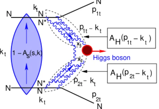
FIG. 1: Survival probability for exclusive central diffractive produc-tion of the Higgs boson
IV. SURVIVAL PROBABILITIES
In the following we shall limit our discussion to the sur-vival probability of Higgs production in an exclusive central diffractive process, calculated in our model. For a general re-view see Ref.[1].
In our model we assume an input Gaussianb-dependence also for the hard diffractive amplitude of interest. Its input, when convoluted with the soft (i,k) channel, is
ΩHi,k=νHi,k(s)ΓHi,k(b), (IV.14)
νHi,k=σHi,k0(s s)
∆H, (IV.15)
ΓHi,k(b) = 1 πRHi,k2
e
− b2 RHi,k2
. (IV.16)
The structure of the survival probability expression is shown in Fig. 1. The corresponding general formulae for the calculation of the survival probability for diffractive Higgs bo-son production have been discussed in Refs.[1, 5, 6]. Accord-ingly,
h|S|2i=N(s)
D(s), (IV.17)
N(s) =R
d2b1d2b2{AH(s,b1)AH(s,b2)
(1−AS(s,(b1+b2)))}2, (IV.18)
D(s) =R
d2b
1d2b2{AH(s,b1)AH(s,b2)}2. (IV.19)
As denotes the soft strong interaction amplitude given by
Eq. (II.5). Using Eq. (II.7)-Eq. (II.9), the integrands of Eq. (IV.18) and Eq. (IV.19) are reduced by eliminating com-mons-dependent expressions.
N(s) =
Z
d2b1d2b2{(1−ael(s,b))AppH(b1)AppH(b2) −asd(s,b)
³
AHpd(b1)AHpp(b2) +AppH(b1)AHpd(b2) ´
−add(s,b)AHpd(b1)AHpd(b2)}2, (IV.20)
D=
Z
d2b1d2b2{AHpp(b1)AppH(b2)}2. (IV.21) Following Refs.[1, 2] we introduce two hardb-profiles
AHpp(b) = Vp→p 2πBHelexp
µ
− b
2
2BHel
¶
, (IV.22)
AHpd(b) = Vp→d 2πBH in
exp µ
− b 2
2BH in
¶
. (IV.23)
The hard radiiRHi,k2 and cross section coefficientsVp→p and
Vp→d are constants derived from HERAJ/Ψelastic and
in-elastic photo and DIS production[12, 13] (see, also, Ref.[6]). BH
el=3.6GeV−2,BinH =1GeV−2,Vp→p=
√
3 andVp→d=1.
have been taken from the experimental HERA data onJ/Ψ production in HERA[12, 13].
Using Eq. (IV.17)-Eq. (IV.21) we calculate the survival probability S2H for exclusive Higgs production in central diffraction. S2H has been calculated[1] in the two amplitude Model A. The resultingS2
H =0.027 is essentially the same
as the predictions of KMR[15]. Our present results, obtained in the three amplitude B Models, indicate a reduction of the output value ofSH2. Its LHC value in Model B(1) is 0.02, and in Model B(2) it is 0.007. We note that, our Model B(1) result is compatible with the result of Ref.[15]. We shall return to this issue in the Discussion Section.
V. AMPLITUDE ANALYSIS
The basic amplitudes of the GLM two channel model are A1,1,A1,2andA2,2, whosebstructure is specified in Eq. (II.5)). These are the building blocks with which we construct ael,
asd andadd (Eq. (II.7)-Eq. (II.9)). The Ai,k amplitudes are
bounded by the black disc unitarity bound of unity. Check-ing Table 1, it is evident that in both Model B(1) and B(2) Ω2,2 is much larger than the other two fitted opacities. As a consequence, the amplitudeA2,2(s,b)reaches the unitarity bound of unity at low energies. Similarly, the output am-plitudeA1,2(s,b)of Model A reaches unity at approximately LHC energy. The observation that one, or even two, of our Ai,k(s,b)=1 does not imply that the elastic scattering
b in fm
a
el
LHC
Tevatron 500 TeV
250 TeV
60 TeV
0 0.1 0.2 0.3 0.4 0.5 0.6 0.7 0.8 0.9 1
0.5 1 1.5 2 2.5 3
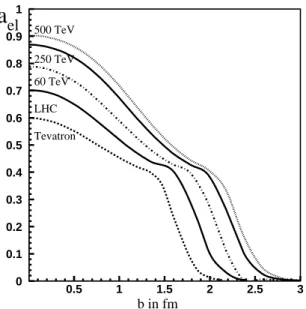
FIG. 2: b dependence ofaelin Model B(2) at different energies
ael(s,b)reaches the black disc bound when, and only when,
A1,1(s,b)=A1,2(s,b)=A2,2(s,b)=1. In such a case we also ob-tain, thatasd(s,b)=add(s,b)=0. This result is independent of
the fitted value ofβ.
Model B(2) predictions ofaelover a wide range of energies
are presented in Fig. 2. A fundamental feature of Models A, B(1) and B(2) is thatael approaches the black disc bound at
b=0 very slowly, reaching the bound at energies higher than the GZK knee cutoff. If correct, this feature implies thatael does not reach the black disc bound over the entire accessible spectrum of Cosmic Rays energies, even though it gets mono-tonically darker.
The explanation of this behavior, in our presentation, is simple. Checking the values ofβ andσ0
i,k corresponding to
the 3 models (see Table 1), we note thatΩ1,1 is smaller by 1-3 orders of magnitude relative toΩ2,2(Ω1,2in Model A). The consequentaelcan reach the black disc bound only when
Ω1,1is large enough so thatA1,1approaches unity.Ω1,1grows slowly likeW0.3 (modululnW). Hence, the slow approach ofaeltoward the black disc bound. This result is
incompati-ble with the output of Ref.[15] in whichaelreaches the black
disc bound approximately at the LHC. In our presentation it implies that unlike our models, in the KMR model there is rel-atively small variance in the weights of the 3 components of the proton wave function.
A consequence of the inputΩi,k being large at smallb, is
that PiS,k(s,b) is very small at b = 0 and monotonically ap-proaches its limiting value of 1, in the highblimit. As a result, given a diffractive (non screened) input, its output (screened) amplitude is peripheral inb. This is a general feature, com-mon to all eikonal models regardless of their b-profiles details. The same is, true, also, with regard to diffractive Good-Walker channels, which are contained inΩi,k. This implies a non
triv-ialtdependence ofdσdi f f(M2di f f)/dt in the diffractive
chan-nels. These qualitative features are induced by Model A, B(1) and B(2), even though their detailed behavior are not identi-cal. Given the deficiencies of our b-profiles, we refrain from giving any specific predictions besides the general observation stated above.
The general behavior indicated above becomes more ex-treme at ultra high energies, when ael continues to expand
and gets darker. Consequently, the inelastic diffractive chan-nels becomes more and more peripheral and relatively smaller when compared with the elastic channel. At the extreme, whenael(s,b)= 1,asd =add =0. We demonstrate this
fea-ture and its consequence at the Planck mass in Fig. 2. As the black core ofaelexpands, the difference between Models
A, B(1) and B(2), considered in this paper, diminishes, being confined to the narrowbtail whereael(s,b)<1. The above
observations may be of interest in the analysis of Cosmic Ray experiments.
VI. DISCUSSION
It is interesting to compare our model and its output with a different eikonal model recently proposed by KMR[14] extending earlier versions[15]. The two models were con-structed with very similar goals but are fundamentally differ-ent in their conceptual theoretical input, data analysis and out-put results.
1) The input of KMR is a conventional Regge model in which high mass diffraction, initiated by Pomeron enhanced dia-grams, is included. GLM is a phenomenological parametriza-tion in which we assume diffracparametriza-tion to be strictly Good-Walker type, with no high mass diffraction distinction. We formulate our input in a general form consistent with Regge, but not exclusively so. Our statistically preferred non factor-izable Model B(2) is compatible with a partonic interpretation which considers the soft ”Pomeron” to be a lowQ2high den-sity limit of the hard Pomeron[11]. The GLM ”Pomeron” is not a Regge simple J-pole, it does not include Pomeron en-hanced diagrams, which are essential in the construction of KMR.
2) Since multi-Pomeron vertices are included in KMR, they had to fixα′=0. In order to maintain the experimentally observed forwardt-cone shrinkage, they constructed a high absorption eikonal model in which the input is non conven-tional∆=0.55. With this input, KMR obtain an approxi-mate DL behavior[16] in the ISR-Tevatron range. However, at higher energies their effective∆ becomes monotonically smaller (its value in the Tevatron-LHC range is reduced to 0.04) which results in a very slow rise ofσtot andσel. GLM
is a weak screening eikonal model. Its fitted input is∆=0.15 andC=α′=0.17. With this input, GLM total cross sections
contribu-tion of the secondary Regge sector. This limited data base is not sufficient to adjust the ”Pomeron” free parameters. GLM chose, therefore, to construct a model containing also the sec-ondary Regge sector and fit the extended data base spanning the ISR-Tevatron energy range. KMR constrain their param-eter adjustment to the small data base of the highest energies. In our opinion the KMR procedure is not adequate. Indeed, their reconstruction of dσeldt at the 3 highest available energies is remarkably similar to a fit they made a few years ago with different parameters, notably a conventional∆input.
4) GLM and KMR determine their input opacities in com-pletely different procedures which define their (different) data bases. GLM approach is a model which takes into account diffractive re-scatterings of the initial projectiles to reconstruct properly the diffractive cross sections, which are, thus, in-cluded in its fitted data base. KMR goal is to reconstruct ael(s,b)for which the diffractive components are needed. To
this end they fit ddtσel neglecting an explicit fit of the diffrac-tive channels. Obviously, combining both GLM and KMR data bases is advisable. Regretfully, we were unable to ob-tain good simultaneous reproduction of such an extended data base. The question, is thus, which model provides a better ap-proximation for the input opacities.
5) The b-distributions of ael(s,b) in GLM are significantly
different from KMR. GLM obtains a relatively wide b dis-tribution compared with a narrower one in KMR.ael(s,b=0)
in KMR is consistently larger than in GLM, approaching the black disc bound much faster than in GLM. Regardless of these differences, the corresponding values ofσtot andσel in
both models in the UA4-Tevatron range are compatible. Such compatibility can exist only over a relatively narrow energy band and it cannot persist over a wide energy range. Indeed, the two models have different LHC and Cosmic Rays predic-tions, which hopefully will be tested soon. Our inability to reproduce dσel
dt outside the narrow forwardt cone implies a
deficiency in our ael at large b. It is not clear if this
defi-ciency is reponsible for the smallSH2 obtained in our Model B(2). Note, that even though our factorizable Model B(1) has the same feature of spurious dips outside the very forward att cone, its predictedS2
His 0.02 which is compatible with KMR.
6) In our opinion, the data adjustment procedure adopted by KMR are not adequate. Our approach is to quantify our fit by minimizing itsχ2. KMR rejects any statistical approach to their data analysis. They tune many of their parameters by eye and refrain from a quantified assessment of their output. The difference between the procedures adopted by the two groups is cardinal, as one is unable to make a systemic evaluation of the KMR output.
7) The difference between the S2H predictions of GLM and KMR are intriguing and reflects the sensitivity of S2H to each model input. S2
H is calculated as a convolution of the
hard amplitude for Higgs production and the soft probability PiS,k(s,b). The hard amplitude features needed for this cal-culation in our model are the hard slopes BHel, BHinand cross section coefficientsVp2→pVp2→d, determined from the HERA measured[12, 13] inJ/Ψphoto and DIS elastic and inelastic production. Our sensitivity to these parameters is shown in
S
2(LHC) in %
BHel(GeV -2
)
BHin
0.5 GeV-2
1 GeV-2
1.5 GeV-2
0 0.5 1 1.5 2 2.5 3 3.5 4 4.5
3.5 4 4.5 5 5.5 6 6.5 7
FIG. 3: The dependence ofS2at the LHC onBH
elandBHin, the slopes
for the hard cross sections.
Fig. 3. Note that when we change the value ofBHin, we keep the ratioVp2→d/BH
inunchanged. Doing so we do not change the
cross section of the reactionγ+p→J/Ψ+X(M≤1.6 GeV). KMR calculation is simpler in as much as they consider just the elastic hard slope. In our opinion there is a gap between the sophistication of KMR soft model and the simplicity of their hard approximation. SinceS2His obtained from a convo-lution of the two terms it is not clear what is the contribution of KMR hard term to the margin of error in their calculation ofS2H.
KMR estimate its margin of uncertainty to be a factor of 2.5. Since our uncertainty derives from similar, though not identical, sources, our assessment is similar. As we saw, both GLM and KMR models are partially deficient. We noted that these are based on the different conceptual constructions and data analysis procedures of the two models. A discrimina-tion between the two models depends on experimental results which are expected to become available within the next few years. In the following we list a few:
1) GLM predictions for σtot and σel at the LHC are 20%
higher than the corresponding KMR values. This is a fun-damental difference since the output energy dependence of GLM, which is a weak screening model, is compatible with an effective∆=0.08 all through the Tevatron-GZK energy range. In the KMR model the effective∆is reduced rapidly due to the very strong screening which is inherent to this model. Hence, the KMR cross sections grow very moderately above the Tevatron energy.
differences are very significant for the DD channel where the KMR prediction at LHC is almost a factor of 3 larger than GLM. Note, that since diffraction in GLM is Good-Walker type, our predicted elastic and diffractive cross sections sat-isfy the Pumplin bound[17], σel(s,b) +σdi f f(s,b)≤ 12σtot.
This bound does not apply to KMR, in which a significant part of its diffractive cross section originates from Pomeron enhanced contributions.
4) An estimate ofS2H value can be obtained, at an early stage of LHC operation, through a measurement of the rate of cen-tral hard LRG di-jets production (a GJJG configuration)
cou-pled to a study of its expected rate in a non screened pQCD calculation.
Acknowledgments
This research was supported in part by the Israel Science Foundation, founded by the Israeli Academy of Science and Humanities, by BSF grant # 20004019 and by a grant from Israel Ministry of Science, Culture and Sport and the Founda-tion for Basic Research of the Russian FederaFounda-tion.
[1] E. Gotsman, E. Levin, U. Maor, E. Naftali, and A. Pry-garin,”HERA and the LHC Proceedings Part A”(2005) 221. (arXiv:hep-ph/0511060[hep-ph]).
[2] E. Gotsman, E. Levin, and U. Maor, arXiv:0708.1506v2[hep-ph].
[3] E. Gotsman, E. Levin, and U. Maor, Phys. Rev. D49, (1994) R4321.
[4] E. Gotsman, E. Levin, and U. Maor, Phys. Lett. B452, (1999) 387.
[5] E. Gotsman, E. Levin, and U. Maor, Phys. Rev. D60, 094011 (1999).
[6] E. Gotsman, H. Kowalski, E. Levin, U. Maor, and A. Prygarin, Eur. Phys. J. C47, 655 (2006).
[7] E. Gotsman, A. Kormilitzin, E. Levin, and U. Maor, Eur. Phys. J. C52, 295 (2007).
[8] J. D. Bjorken, Int. J. Mod. Phys. A7, 4189 (1992); Phys. Rev. D47, 101 (1993).
[9] E. Gotsman, E. M. Levin, and U. Maor, Phys. Lett. B309, 199 (1993).
[10] T. Affolderr et al., Phys. Rev. Lett.87, 141802 (2001). [11] J. Bartels, E. Gotsman, E. Levin, M. Lublinsky, and U. Maor,
Phys. Rev. D68, 054008 (2003); Phys. Lett. B556, 114 (2003). [12] H.Kowalski and D. Teaney, Phys. Rev. D68, 114005 (2003). [13] ZEUS Collaboration, Nucl. Phys. B695, 3 (2004); Eur. Phys.
J. C24, 345 (2002).
[14] V. A. Khoze, A. D. Martin, and M. G. Ryskin, Eur. Phys. J. C 54, 199 (2008).
[15] V. A. Khoze, A. D. Martin, and M. G. Ryskin, Eur. Phys. J. C 18, 167 (2000); Phys. Lett. B643, 93 (2006).
[16] A. Donnachie and P.V. Landshoff, Nucl. Phys. B 231, 189 (1984); Phys. Lett. B296, 227 (1992).