Application of Artificial Neural Network for Seasonal Rainfall Forecasting: A Case Study for South Australia



Abstract— Quantitative approaches are very useful tools in

forecasting purposes among the hydrologists for enhanced decision making. Modelling accuracy is also another important aspect in selecting an appropriate forecasting technique. Compared to other regions, South Australia’s seasonal rainfall forecasting models were not very accurate and satisfactory in regards to their forecasting skills. Past studies conducted on South Australia’s rainfall variability have mostly used the linear methods and showed very low rainfall predictability through the individual effects of the concurrent climate predictors. Previous research had not considered the interactions/effects of multiple combinations (more than two) of the climate modes at a time in order to forecast rainfall across South Australia (SA). Moreover, lagged-time influences of the potential climate indices on rainfalls were ignored. Therefore, SA has been chosen as a case study to fill up the present research gap. The relationships among the rainfall and climate predictors are not linear; therefore in order to improve the predictability of rainfall multivariate non-linear Artificial Neural Networks (ANN) technique was used in this study. Seasonal rainfall is being forecasted with the effect of past values of the potential climate predictors such as El Nino southern Oscillation (ENSO), Southern Annular Mode (SAM) and Indian Ocean Dipole (IOD) by developing non-linear ANN models. The non-linear artificial intelligence technique, ANN has already been proved superior compared to other techniques in other regions of Australia. However, previously it has not been attempted for SA. In order to compare the forecasting ability by the ANN models, Multiple Linear Regression (MR) models were developed as a benchmark. Results revealed the superiority of multivariate non-linear ANN over traditional linear MR methods for seasonal rainfall forecasting by considering the effects of climate variables.

Index Terms—Artificial Neural Network (ANN), rainfall

forecasting, climate predictors, ENSO, IOD, SAM

I. INTRODUCTION

OR design, planning and development of water resources management strategies, rainfall forecasting is essentially important. It helps to evaluate the water balance between future supply and availability, which ensures proper strategic management of water resources. Rainfall is

Manuscript received March 29, 2016; revised April 7, 2016.

H. M. Rasel is a PhD student of the Department of Civil and Construction Engineering, at Swinburne University of Technology, Melbourne, VIC 3122, Australia. (Telephone: +61392145630; e-mail: hrasel@swin.edu.au).

M. A. Imteaz is an Associate Professor with the Department of Civil and Construction Engineering, at Swinburne University of Technology, Melbourne, VIC 3122, Australia. (e-mail: mimteaz@swin.edu.au).

the most studied

and most important hydro-climate variables among the climatologists all over the world because of its significance in sustainable water resources management, agricultural activities and ecological management. Therefore, rainfall forecasting several months or seasons has become one of the primary goals of the water resources managers for many decades. Many researchers have tried to establish the relationships between large-scale climate drivers and rainfall in different parts around the world using different linear and non-linear methods [1]. Reliable rainfall forecasting could be beneficial in the management of land, watershed and water systems [2], especially in Australia, where the hydroclimatic variability is extremely high [3]. Global climate change is predicted to increase the rainfall variability which will only exacerbate the water-related issues [4]. Australia is exposed to severe floods and droughts; therefore seasonal rainfall forecasting will be very helpful for water resources management, food production and mitigating flood risks.

The rainfall over Australia is extremely variable that varies both spatially and temporally. It is well established that the rainfall variability in Australia has been accompanied with several oceanic-atmospheric processes, which are classified by several remote climate modes/variables and in many parts of Australian rainfalls are significantly affected these remote climate variables [5]. The most important influence is thought to be from the tropical Pacific Ocean driver, i.e. the ENSO [6, 7]. It has been established that the climatic influences from the Indian Ocean also plays a vital role in rainfall variability in Australia which is known as IOD [6, 8]. Another important climate variable originating from the Southern Ocean is called SAM [9-11]. Several studies have tried to explore the association of climate predictors with the Australian rainfalls. Some of the past studies on hydro-climatic variability were generally focused on overall Australia [6, 10-11]. Some of the researches focused particularly on Eastern and South Eastern Australia [12-17]; whereas others were more concentrated on other regions such as South West Western Australia [18, 19].

However, very limited studies were found especially focusing on the variability of South Australian rainfall in association with the remote climate variables [6, 9, 20-22].

Application of Artificial Neural Network for

Seasonal Rainfall Forecasting: A Case Study for

South Australia

Therefore further study is required to explore the relationships between the potential large scale remote climate drivers and SA’s seasonal rainfalls to develop a reliable seasonal rainfall forecast model. To date, the studies being conducted on South Australian rainfall variability have used linear methods, though a recent study has considered non-linear threshold method for the same purpose but still failed to achieve the significant outcome due to the basic limitation of this method. In Australian climate at any particular locations, any individual climate index may explain only about 20% of the rainfall variability [23]. In another study [6] investigated the relationship between climate drivers and overall Australian rainfall and concluded that individual climate drivers can explored up to 20% variability of South Australian rainfall. Reference [6] used ENSO and SAM in their study as individual climate index respectively and explored that only a single climate index might not be sufficient to determine the maximum correlations between these climate features and rainfall.

Recently, Reference [20] used the non-linear threshold method for investigating the variability and forecasting capability of South Australian seasonal rainfall with the aid of climate predictors where maximum of two climate drivers were used instead of single and found some successes regarding correlations and rainfall variability. Reference [20] suggested that the seasonal rainfall variability skill is largely depends on the influences and association of the multiple combination (more than two at a time) of climate drivers. However, there was a basic drawback of threshold method used in their study; it was not able to explore the complex rainfall-climate predictor’s relationships with the combinations of more than two climate drivers due to the limitations of this method. Because, the threshold method applied in the study was unable to derive mathematical model involving more than two climate drivers at a time. Reference [20] also suggested that a new statistical non-linear multi-variate ANN approach which is free from such limitations of input variables should be used with the threshold method in using the number of combinations of input variables at a time. Some studies have already shown that the multivariate non-linear ANN technique is able to map the complex rainfall-climate driver’s relationships with higher predictability compared to the threshold method used in the study of [20]. Such an emerging non-linear artificial intelligence technique was very rarely used for rainfall forecasting purposes in Australia using the large scale climate drivers as potential predictors. Few studies found are limited to some particular regions of Australia including the Queensland [14] and Victoria [5, 12-13]. For Victorian rainfalls, ANN models were developed for the seasonal rainfall forecasting and the ANN outputs were found to be superior compared to other techniques [5, 12-13].

So far, no study has established rainfall forecasting model for South Australia using the non-linear multivariate ANN approach considering multiple combinations (more than two) of potential climate variables. Moreover, the current model outputs will be deterministic meaning that it can explore with quantitative forecasting, in opposed to

probabilistic forecast that usually gives results only above or below median value.

II. DATA AND METHODS A. Rainfall and Climate predictor variables data

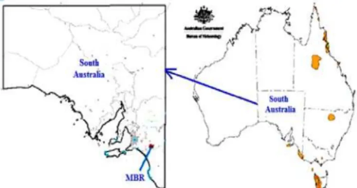
The historical monthly rainfall data was obtained from the Australian Bureau of Meteorology website. As a case study of South Australia, Mount Bold Reservoir (MBR) rainfall station has been chosen. Figure 1 shows the location details of the rainfall station considered in this study. Seasonal spring (September-October- November) rainfall was obtained from monthly rainfall data from January 1957 to December 2013 (www.bom.gov.au/climate/data/). The monthly values of Nino3, Nino3.4, Nino4 and SOI were used as the representation of ENSO climate predictor variables. A measure of IOD is the Dipole Mode Index (DMI) from the Indian Ocean and SAM climate index from the Southern Ocean were considered. ENSO, IOD and SAM indices were obtained from Climate Explorer website http://climexp.knmi.nl/. A robust multivariate non-linear Artificial Neural Network (ANN) modelling technique will be used as a new technique to accomplish the goal of this study. In order to compare the forecast skill of non-linear ANN models, traditional Multiple Linear Regression (MR) linear models were used as a benchmark.

Fig. 1. Map showing the study area with selected location as a case study (Source: www.bom.gov.au).

B. Artificial Neural Networks

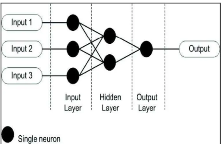
The Artificial Neural Network (ANN) approach is a non-linear statistical technique that has become popular among scientists as an alternative technique for predicting and modelling complicated time series, weather phenomena and climate variables (Mekanik et al., 2013). ANN has been used in many hydrological and meteorological applications; it has also been used for many cases of rainfall forecasting [24-26]. The parameters for ANN modelling are basically network topology, neurons characteristics, training and learning rules. A typical architecture and working layout of an artificial neural network (ANN) is shown in the figure 2.

in a MLP since they provide the nonlinearity between the input and output sets.

Fig. 2. Typical architecture and working layout of an artificial neural network (ANN).

Mathematically, the network illustrated in figure 2 can be expressed by using the following equation:

Where, Yt is the output of the network, xi is the input to the network, wi and wj are the weights between neurons of the input and hidden layer and between hidden layer and output respectively; f1 and f2are the activation functions for the hidden layer and output layer respectively. In this study f1 is considered tansigmoid function which is a nonlinear function and f2 is considered the linear purelin function. The ANN models were trained based on Levenberg-Marquardt algorithm. Number of hidden neurons was chosen based the on trial and error procedures considering the different number of hidden nodes.

C. Multiple Regression Modelling

Multiple Regression (MR) is a linear statistical modelling technique that predicts a dependent or predictant variable based on the several other independent or predictor variables through the least square method. MR model can be presented by using the following general equation:

Where,

Y= Dependent variable (spring rainfall)

X1= First independent variable or predictor (i.e. ENSO representative)

X2= Second independent variable or predictor (i.e. SAM, IOD representatives)

b1= Coefficient of first independent variable, X1 b2= Coefficient of second independent variable, X2 a= Constant or intercept

c= Error

The models were evaluated using Pearson correlation (R), root mean square error (RMSE), and index of agreement (d), which is widely used for the evaluation of prediction model. The optimum value of d is 1 is considered the better

model meaning that all the modelled values fit the observations [27]. The correlations which are statistically significant at 1 and 5% levels were considered in this study.

III. RESULTS AND DISCUSSIONS

This study attempts to model the seasonal spring rainfall which includes September, October and November (S-O-N). For this purpose, from December to August month’s Nino3, Nino3.4, Nino4, SOI, DMI and SAM climate predictor’s variables have been selected to be used in the non-linear ANN and linear MR modelling of seasonal spring rainfall (S-O-N). Thus, the single linear correlations of these months’ (December to August) climate variables with Mount Bold Reservoir (MBR) rainfall were calculated and the months with highest significant correlation were chosen to be used in the modelling which is shown in table I. It can be seen that not all the lags have significant relationship with rainfall; the maximum correlation of 0.44 is achieved for DMI-August. For different indices different months have significant relationship with rainfall, however July and August months are having the highest correlation with rainfall. It was observed that the maximum three months’ (June, July and August) lagged SOI, DMI and SAM climate predictors have significant correlation with spring rainfall.

TABLE I

SIMPLE LINEAR CORRELATION OF SEASONAL SPRING RAINFALL AND DIFFERENT LAGGED-TIME INFLUENCES OF INDIVIDUAL CLIMATE PREDICTORS (CORRELATIONS AT EITHER 1 OR 5% SIGNIFICANT LEVELS ARE

SHOWN WITH ASTERISK)

Month Pearson correlation with individual climate predictors

DMI SOI SAM

Dec --- --- ---

Jan --- --- ---

Feb --- --- ---

Mar --- --- ---

Apr --- --- ---

May --- --- ---

June --- --- -0.33*

July -0.38** 0.33* ---

Aug -0.44* --- ---

used to forecast seasonal rainfall with correlation 0.56 which is the improvement of linear MR model by 44% with the combination of maximum two climate predictors. Attempts have been made to use all the possible combined lags as predictors in MR modelling, but most of the combined-lagged predictor’s model was not statistically significant. Therefore, those insignificant models were not reliable in rainfall forecasting. Even though some of the lags of the predictors were not linearly correlated with the rainfall, however for non-linear ANN modeling all the lagged indices were used as predictors (Dec. to Aug.). The reason behind of taking all these lags due to the concept of ANN which is capable of finding the nonlinear relationship between the predictors and rainfall. Table II shows the result of non-linear ANN modeling on both training-validation and testing set using the combination of two as well as multiple climate predictor’s model to figure out the best combination of the forecasting model. The number of hidden neurons giving the least error, maximum correlation as well as maximum data agreements between observed and modelled rainfall was 4.

TABLE II

COMPARISON BETWEEN THE CORRELATIONS OF SEASONAL SPRING RAINFALL WITH LINEAR AND NON-LINEAR MODELS Combine

d models

Correlation Training-Validatio

n

Testin

g Training-Validatio n

Testin g

Linear Regression

model Non-linear ANN model

DMI-SAM 0.46 0.56 0.62 0.82

SOI-SAM 0.45 0.34 0.70 0.41

DMI-SOI-SAM Model is not able to explain the multiple combination of

variables

0.75 0.93

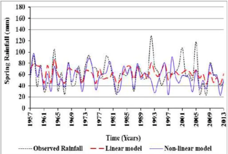
Multivariate non-linear ANN models are showing much higher correlations and statistical performances for both the combination of two and three climate predictors’ models. The correlation in ANN models are significantly higher than the maximum correlation found in MR models, which was 0.56. However using ANN approach the correlations were improved significantly using combination of two climate predictors which is found 0.82, the improvement of ANN model was observed by 46%. Further analyses with the non-linear ANN model was carried out by using three climate predictors (i.e. DMI-SOI-SAM), which was the basic input limitations in linear models. The results demonstrated further improvement of the forecasting ability of the multivariate ANN methods and the correlation was found up to 0.93, which is a significant improvement (by 66%) over the correlation achieved by the best liner regression model incorporating two predictors. Figure 3 shows the comparisons of observed and predicted rainfalls using linear MR and non-linear ANN models. It can be seen that the MR models is modeling around the mean of the series and is not capable of capturing the peaks and minimum values. On the other hand ANN is smoothly fitting the series capturing

most of the peaks and minimum values.

Fig. 3. Comparison between non-linear ANN model with linear model’s output for spring rainfall, (1957-2008=training-validation period, 2009-2013=testing period)

The Index of agreement (d) an additional criterion has been chosen for model comparison and for the better assessment of the model’s performance (Willmott, 1981). It is seen from table III that non-linear ANN revealed the least error and better fitted model regarding RMSE and ‘d’.

TABLE III

EVALUATION OF MODEL PERFORMANCE USING ‘RMSE’ AND ‘d’ VALUES FOR THE BEST MODELS

Models Model Performance

Training-Validation Testing Training-Validation Testing

Linear Regression

RMSE d

DMI-SAM 20.91 11.95 0.59 0.70

SOI-SAM 21.00 13.36 0.56 0.46

DMI- SOI-SAM

--- --- --- ---

Non-linear

ANN DMI-_SAM 16.35 9.04 0.72 0.81

SOI-SAM 15.82 14.64 0.61 0.59

DMI- SOI-SAM

14.06 8.04 0.67 0.93

Therefore, depending upon the correlation and model’s RMSE and d values, ANN models output with the multiple combinations such as DMI-SOI-SAM is the better predictors of SA’s seasonal rainfall. The second most reliable ANN models output is obtained using DMI-SAM combinations. Therefore, it seems that DMI and SAM is more reliable rainfall predictors than other indices affecting South Australian seasonal rainfalls significantly.

IV. CONCLUSIONS

lagged DMI-ENSO-SAM climate combinations. Previous studies were focusing on finding the effect of these climate indices individually on SA’s rainfalls and were unable to achieve the rainfall predictability with good statistical correlations. ANN models have shown to be an effective, general-purpose approach for pattern recognition, classification, clustering, and especially time series prediction with a high degree of accuracy. This study elaborated the improvement of the generalization ability of complex relationships between rainfall and climate predictors by using the multi-variate non-linear ANN modelling approach in predicting the seasonal rainfall in South Australia.

The traditional linear MR model using combined predictors (DMI-SAM) was found to provide the maximum correlation of 0.56, which is an improvement of model correlations by 44% compared to linear models’ performances using single predictor. The attained correlations of ANN models are significantly higher than the maximum correlation found in MR models (R= 0.56). Using ANN approach the correlations were improved significantly; with the combination of two climate predictors (DMI-SAM) the maximum correlation found was 0.82 (an improvement of 46% compared to MR model using two predictors) and with the combination of three predictors (DMI-SOI-SAM) the maximum correlation achieved was 0.93 (an improvement of 66% compared to MR model using two predictors). ANN with combined-lagged climate predictors was able to model the observed rainfall in a way that the models can predict the pattern of rainfalls several months in advance with very good accuracy (least error and model correlation up to 0.93). Therefore, depending upon the correlation as well as other model performances evaluation parameters such as RMSE and d values, ANN model output with the multiple combinations of predictors (DMI-SOI-SAM) is the best model for the predictions of SA’s seasonal rainfall compared to any other available technique/model. This study concluded that non-linear artificial intelligence modelling technique is able to provide higher correlations and lower error to forecast rainfall compared to linear methods and it would be a suitable prediction tool for the prediction of South Australian spring rainfall. There is a need to further investigate this method on other rainfall stations in this region to generalize the forecasting model which will be covered in future studies.

REFERENCES

[1] Shukla, R. P., Tripathi, K. C., Pandey, A. C., & Das, I. M. L. “Prediction of Indian summer monsoon rainfall using Niño indices: A neural network approach,” Atmospheric Research, Vol. 102 No. 1-2,

pp. 99-109, 2011.

[2] Anwar, M. R., Rodriguez, D., Liu, D. L., Power, S., O’leary G. J. “Quality and potential utility of ENSO-based forecasts of spring rainfall and wheat yield in south-eastern Australia,” Australian Journal of Agricultural Research, vol. 59, pp. 112–126, 2008.

[3] Peel, M. C., T. A. McMahon, and Finlayson, B. L. “Variability of Annual Precipitation and Its Relationship to the El Nino-Southern Oscillation,” Journal of Climate, vol. 15, no. 5, pp. 545-551, 2002.

[4] Yilmaz, A.G., Hossain, I. and Perera, B.J.C. “Effect of climate change and variability on extreme rainfall intensity–frequency–duration relationships: a case study of Melbourne,” Hydrology Earth System Sciences, vol. 18, pp. 4065-4076, 2014.

[5] Mekanik, F. and Imteaz, M. A. “Forecasting Victorian spring rainfall using ENSO and IOD: A comparison of linear multiple regression and nonlinear ANN,” in 2nd International Conference on Uncertainty Reasoning and Knowledge Engineering, Jakarta, August 2012, pp.

1-5.

[6] Risbey, J. S., Pook, M. J., McIntosh, P. C., Wheeler, M. C., Hendon, H. H. “On the remote drivers of rainfall variability in Australia,”

Monthly Weather Review, vol. 137, no. 10, pp. 3233-3253, 2009.

[7] Power, S., Casey, T., Folland, C., Colman, A. and Mehta, V. “Inter-decadal modulation of the impact of ENSO on Australia,” Climate Dynamics, vol. 15, no. 5, pp. 319-324, 1999.

[8] Verdon, D. C., and Franks, S. W. “Indian Ocean sea surface temperature variability and winter rainfall: Eastern Australia,” Water Resources Research, vo. 41, no. 9, pp. 1-10, 2005.

[9] Chowdhury, R. K., Beecham, S. “Influence of SOI, DMI and Niño3.4 on South Australian rainfall,” Stochastic Environmental Research and Risk Assessment, vol. 27, no. 8, pp. 1909–1920, 2013.

[10] Kirono, D. G. C., Chiew, F. H. S., Kent, D. M. “Identification of best predictors for forecasting seasonal rainfall and runoff in Australia,”

Hydrological Processes, vol. 24, no. 10, pp. 1237-1247, 2010.

[11] Meneghini, B., Simmonds, I., Smith, I. N. “Association between Australian rainfall and the Southern Annular Mode,” International Journal of Climatology, vol. 27, no. 1, pp. 109-121, 2007.

[12] Mekanik, F., Imteaz, M. A., Gato-Trinidad, S. and El-Mahdi, A. “Multiple regression and Artificial Neural Network for long-term rainfall forecasting using large scale climate modes,” Journal of Hydrology, Vol. 503, pp. 11-21, 2013.

[13] Mekanik, F. and Imteaz, M. A. “Capability of Artificial Neural Networks for predicting long-term seasonal rainfalls in east Australia,” in 20th International Congress on Modelling and Simulation (MODSIM), Adelaide, December 2013, pp. 2674-2680.

[14] Abbot, J. & Marohasy, J. “Application of artificial neural networks to rainfall forecasting in Queensland, Australia,” Advances in Atmospheric Sciences, vol. 29, no. 4, pp. 717-730, 2012.

[15] Kiem, A. S., and Verdon-Kidd, D. C. “Climatic drivers of Victorian streamflow: Is ENSO the dominant influence?,” Australian Journal of Water Resources, vo. 13, no. 1, pp. 17-29, 2009.

[16] Murphy, B. F. & Timbal, B. “A review of recent climate variability and climate change in southeastern Australia,” International Journal of Climatology, vol. 28, pp. 859-879, 2008.

[17] Verdon, D. C., Wyatt, A. M., Kiem, A. S., Franks, S. W. “Multidecadal variability of rainfall and streamflow: Eastern Australia,” Water Resources Research, vol. 40, no. 10, paper number

W10201, 2004.

[18] Li, F., L. E. Chambers, and Nicholls, N. “Relationships between rainfall in the southwest of Western Australia and near-global patterns of sea-surface temperature and mean sea-level pressure variability,”

Australian Meteorological Magazine, vol. 54, pp. 23-33, 2005.

[19] Ummenhofer, C. C., Sen Gupta, A., Pook, M. J., England, M. H. “Anomalous rainfall over southwest Western Australia forced by Indian Ocean sea surface temperatures,” Journal of Climate, vol. 21,

pp. 5113-5134, 2008.

[20] Tozer, C. R. “Utilising Insights into Rainfall Patterns and Climate Drivers to Inform Seasonal Rainfall Forecasting in South Australia,”

PhD thesis, 2014.

[21] Cai, W., van Rensch, P., Cowan, T., Hendon, H. H. “Teleconnection pathways of ENSO and the IOD and the mechanisms for impacts on Australian rainfall,” Journal of Climate, vol. 24, no. 15, pp.

3910-3923, 2011.

[22] Nicholls, N. “Local and remote causes of the southern Australian autumn-winter rainfall decline, 1958–2007,” Climate Dynamics, vol.

34, no. 6, pp. 835-845, 2010.

[23] Schepen, A., Wang, Q. J., Robertson, D. “Evidence for using lagged climate indices to forecast Australian seasonal rainfall,” Journal of Climate, vol. 25, no. 4, pp. 1230-1246, 2012.

[24] Mekanik, F., Lee, T. S., & Imteaz, M. A. “Rainfall modeling using Artificial Neural Network for a mountainous region in west Iran,” in

Proceedings of the 19th International Congress on Modelling and Simulation ( MODSIM), Perth, Australia, 12–16 December 2011.

[25] Hsu, K., Gupta, H. V., & Sorooshian, S. “Artificial neural network modeling of the rainfall-runoff process,” Water Resources Research,

vol. 31, no. 10, pp. 2517-2530, 1995.

[26] Yilmaz, A. G., Imteaz, M. A. and Jenkins, G. “Catchment flow estimation using Artificial Neural Networks in the mountainous Euphrates Basin,” Journal of Hydrology, vol. 410, pp. 134-140, 2011.

[27] Willmott, C. J. “On the validation of models,” Physical Geography,