FINAL VERSION
Coimbra, Danilo Barbosa
C634m Multidimensional projections for the visual
exploration of multimedia data / Danilo
Barbosa Coimbra; orientador Fernando Vieira Paulovich (ICMC-USP, Brasil); orientador Alexandru Cristian Telea (RUG, Holanda). – São Carlos – SP, 2016.
236 p.
Tese (Doutorado - Programa de Pós-Graduação em Ciências de Computação e Matemática Computacional) – Instituto de Ciências Matemáticas e de Computação,
Universidade de São Paulo, 2016.
1. information visualization. 2. multidimensional projection. 3. multimedia visualization.
VERSÃO REVISADA
First and foremost, I would like to thank my supervisors, Alex Telea and Fernando Paulovich. Alex, thanksfor the long meetings discussing technical and sometimes non-technical subjects. I am truly amazed by the speed of your thoughts and how you can explain their complexity so easily to your students. Also, I wonder how you can preserve your enthusiasm and your good mood in your everyday life, even after a hard working day. Fernando, thanks for thecountless meetingsdiscussing ideasand life, they wereessential to keep memotivated during this period. Also, you showed to me that we can enjoy different life styles, even when working alot. To both, thanks oncemorefor theguidanceand supervision, you havehelped me to reach personal and professional levelsthat wereonly possible in my most optimistic dreams. My dear family: Mom and Dad, I know how hard you both fight to give me this opportunity, thank you. Káand Hugo, thanksfor thekind wordswhen listening to my complaints during this time, and also for going out and have fun with me when I needed to rest my mind. Many thanksto my relativesfrom Patos deMinas, Cuiabá, and Rondonópolisto always encouragemewith my PhD work, and my apologiesfor thetimeI wasabsent.
Maiti-Roliudi, my Brazilian group of roommateswhich I am very proud to be part of: Gabriel, JoséAugusto, Tácito, Maycon, Flávio, Ricardo, Cássio, Léo and Fernando, thanks for all the pleasant moments when drinking, playing, traveling, mailing, and talking about work, politics, soccer, and relationships.
Many thanks to theWinschoterdiep friends, whom I shared many international dinners, talking, drinking, and many otherswonderful moments together, especially: Sven, Alex, Laura F., Nico, Camila, Victor, Antonia, Laura K., Juan, Octavio, Emilia, Stephan, Efthymis, Jelle, Thomas, and Rixt. I am very glad that I got to know all of you.
Thanksto the Brazilian friendsI met in Groningen for thevery relaxing timetogether and the Turkish friends to treat meso nicely and helpful when I had just arrived there. Enrico, I am thankful and glad to haveknown you during this time aswell.
Rafael, aspecial friend, but also acinephile, agamer, asinger, ageek,... Thanks for all thetime since themaster degree, in special our time in Groningen, you and Priscilahelped mea lot there(“Happinessis only real if shared”).
useful (or not) ideas while drinking coffee, and momentsof making fun of each others inside the office. Thanks go to the SVCG research group in Groningen, that treat me kindly and helped me to improve my research skills. Many thanks to the5thfloor JBI friends, for exploring thecity,
countries and restaurants, and spending great moments together. Also, I would liketo acknowl-edge the research funding provided by the Brazilian agencies FAPESP(grant 2011/17925-1), CNPq (grant 156580/2011-0), and theresearch project CAPES/NUFFIC 028/11.
Carol, for believing in memorethan I usually do, giving mesupport in hard times and sharing so many great momentstogether: Thanksa lot.
COIMBRA, D. B.. Multidimensional projections for the visual exploration of multimedia data. 2016. 236f. Thesis(DoctorateCandidate Program in Computer Scienceand Computatio-nal Mathematics(ICMC-USP) and of PhD (RUG), in accordancewith theinternatioComputatio-nal academic agreement for PhD double degreeagreement for PhD double degree signed between ICMC-USP and RUG) – Instituto de Ciências Matemáticas e deComputação (ICMC/USP), São Carlos – SP.
O advento contínuo de novas tecnologias tem criado um tipo rico e crescente de fontes de informação disponíveis para análise einvestigação. Nestecontexto, aanálisededados multidi-mensional éconsideravelmenteimportantequando selidacom grandesecomplexosconjuntos dedados. Dentreaspossibilidadesao analisar esses tiposde dados, aaplicação detécnicasde visualização podeauxiliar o usuário aencontrar eentender ospadrões, tendênciase estabelecer novas metas. Alguns exemplosdeaplicaçõesdevisualização deanálisededadosmultidimen-sionais vão declassificação deimagens, nuvens semânticadepalavras, eanálisedegruposde coleção dedocumentos, àexploração deconteúdo multimídia.
Estateseapresentaváriosmétodosdevisualização paraexplorar deformainterativaconjuntosde dadosmultidimensionaisquevisam deusuáriosespecializadosaoscasuais, fazendo uso deambas representações estáticas edinâmicascriadas por projeçõesmultidimensionais. Primeiramente, apresentamos uma técnica de projeção multidimensional que preserva fielmente distância e que podelidar com qualquer tipo de dadoscom alta-dimensionalidade, demonstrando cenários de aplicações em ambos os casos de multimídia e coleções de documentos de texto. Em seguida, abordamos atarefadeinterpretar asprojeções em 2D, calculando erros devizinhança. Posteriormente, apresentamos um conjunto de visualizações interativas que visam ajudar os usuárioscomessastarefas, revelando aqualidadedeumaprojeçãoem3D, aplicadasemdiferentes cenáriosdealtadimensionalidade. Napartefinal, discutimosduasabordagensdiferentes para obter percepçõessobredadosmultimídia, em particular vídeosde futebol. Enquanto aprimeira abordagem utiliza projeções multidimensionais, a segunda faz uso de uma eficiente metáfora visual para auxiliar usuários não especialistasem navegar eobter conhecimento em partidas de futebol.
COIMBRA, D. B.. Multidimensional projections for the visual exploration of multimedia data. 2016. 236f. Thesis (Doctorate Candidate Program in Computer Science and Compu-tational Mathematics (ICMC-USP) and of PhD (RUG), in accordance with the international academic agreement for PhD doubledegreeagreement for PhD doubledegreesigned between ICMC-USP and RUG) – Instituto de Ciências Matemáticas ede Computação (ICMC/USP), São Carlos – SP.
The continuously advent of new technologies havemadea rich and growing type of information sourcesavailableto analysesand investigation. In thiscontext, multidimensional data analysis is considerably important when dealing with such large and complex datasets. Among the possibilities when analyzing such kind of data, applying visualization techniques can help the user find and understand patters, trends and establish new goals. Some applicationsexamples of visualization of multidimensional dataanalysisgoesfrom image classification, semantic word clouds, cluster analysisof document collection to exploration of multimediacontent.
This thesis presents several visualization methods to interactively explore multidimensional datasets aimed from specialized to casual users, by making use of both static and dynamic representations created by multidimensional projections. Firstly, we present a multidimen-sional projection technique which faithfully preserves distance and can handle any type of high-dimensional data, demonstrating applications scenariosin both multimediaand text docu-ments collections. Next, we address the task of interpreting projections in 2D, by calculating neighborhood errors. Hereafter, we present a set of interactive visualizations that aim to help users with these tasks by revealing the quality of a projection in 3D, applied in different high dimensional scenarios. In thefinal part, weaddress two different approaches to get insight into multimediadata, in special soccer sport videos. While the first make use of multidimensional projections, thesecond usesefficient visual metaphor to help non-specialist usersin browsing and getting insightsin soccer matches.
COIMBRA, D. B.. Multidimensional projections for the visual exploration of multimedia data. 2016. 236f. Thesis(DoctorateCandidate Program in Computer Scienceand Computatio-nal Mathematics(ICMC-USP) and of PhD (RUG), in accordancewith theinternatioComputatio-nal academic agreement for PhD double degreeagreement for PhD double degree signed between ICMC-USP and RUG) – Instituto de Ciências Matemáticas e deComputação (ICMC/USP), São Carlos – SP.
De voortdurendeopmars van nieuwe technologieën hebben een rijk type van informatiebronnen beschikbaar gesteld voor analyse en investigatie. In deze context, multidimensionale dataanalyse is zeer belangrijk wanneer men moet handelen met grote en complexe dataverzamelingen. Tussen de mogelijkheden voor de analyse van dergelijke daa visualisatietechnieken kunnen gebruikers helpen om relevante patronen en trends te vinden en analyseren. Voorbeelden van multidimensionaledataanalyseomvatten beeldclassificatie, semantische ’word clouds’, en clusteranalyses van documentverzamelingen en exploratievan multimediaverzamelingen. Dit proefschrift presenteert verschillendevisualisatiemethodes voor deinteractieveexploratie van multidimensionaledataverzamelingen voor beide gespecialiseerdeen gewone gebruikers, gebaseerd op statische en dynamische representaties gebouwd met multidimensionaleprojecties. We presenteren eerst een multidimensionaleprojectietechniek dieafstanden goed bewaart voor alle types multidimensionale gegevens, met toepassingen in multimedia en text-document verzamelingen. Verder analyseren wij de taak van projectieinterpretatie in 2D gebaseerd op lokale fouten. Verder presenteren wij een groep interactieve visualisaties die de gebruiker in staat stelt om 3D projecties te interpreteren, voor verschillende hoogdimensionale scenario’s. Alslaatst presenteren wij tweeaanpakken om inzicht tekrijgen in multimediagegevens, zoals sport-videos, gebaseerd op multidimensionaleprojecties en ook bijpassendevisuelemetaforen om non-specialistischegebruikers in staat te stellen om voetbalwedstrijden door tebladeren om inzicht tevergaderen.
Figure1 – Exampleof aSPLOM (irisdataset) (WARD; GRINSTEIN; KEIM, 2010). . 52
Figure2 – ExamplePCP visualizationsusing theparvis toolkit (LEDERMAN, 2012). . 54
Figure3 – Examples of PCPvisualizations. . . 55
Figure4 – Examples of radial layout: DataMeadow (ELMQVIST; STASKO; TSIGAS, 2007). SampleDataRosevisualization for a university student databaseof a computer science department. . . 56
Figure5 – Tablelensexample. (a) Zoomed in tablewith text and bar charts. (b) Zoomed out table. (c) Table sorted and grouped on first three columns. (d) Table hierarchy visualized with atreemap. Imagesgenerated with theTableVision tool (TELEA, 2006). . . 57
Figure6 – Comparison of table(a) vs (b) PCPvisualization layouts. Image taken from (TELEA, 2014). . . 58
Figure7 – VisDB (KEIM; KRIEGEL, 1994). Color coding rangesfrom yellow for those data items that better satisfy a posed query to green, blue, red, and almost black for thosefurther away from it. . . 59
Figure8 – Conceptual representation of multidimensional projections for reducing a datatableto a2D scatterplot. . . 61
Figure9 – The top-right window presents the initial point cloud projection generated by LoCH from an imagedataset collected from theinternet (FADEL et al., 2015). The larger image has its thumbnail image instances corresponding with thesamepoint location. . . 65
Figure10 – Comparing projection quality with stress scatterplots. The x axismaps the distanced in theinput high-dimensional space. The y axis maps thedistance d in theembedding low-dimensional space. Imagetaken from (PAULOVICH et al., 2011). . . 66
Figure11 – Visualization of a collection of news using theProjCloud tool (PAULOVICH et al., 2012). . . 68
Figure12 – Visualization of a single tennismatch in TenniVis (POLK et al., 2014). . . . 75
Figure13 – Visual Storylines(CHEN; LU; HU, 2012) . . . 77
freely handling thepointsin aiterativeprocess. c) Remaining instancesare interpolated, taking into account thegeometry given by this initial placement, projecting thewholedataset. . . 83
Figure16 – Dataflow-likepipelinepresenting the components of LAMP. . . 84
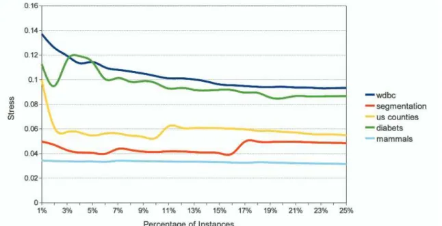
Figure17 – The stress quality metric of LAMP as a function of the number of control points. These range from 1% to 25% of the total point count. Experiments doneon fivedataset (described separately in Table1 for detailsabout thedata sets). . . 88
Figure18 – Boxplots comparing stress of ten techniques, including LAMP. . . 90
Figure19 – Boxplots comparing computational timesof ten techniques, including LAMP. 90
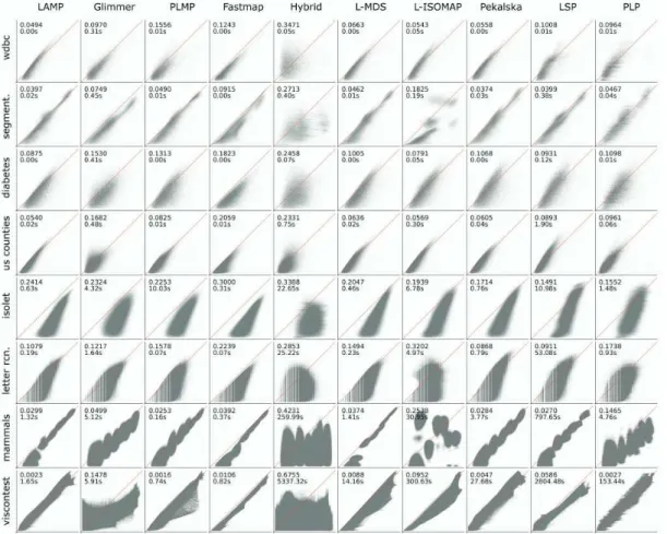
Figure20 – Scatterplots original-distance × projected-distance of ten techniques, includ-ing LAMP. . . 91
Figure21 – LAMP, LSP, Pekalska and PLMPprojections when the user manipulated the control points. . . 93
Figure22 – LAMP projection when varying the percentageof nearest control points. . . 93
Figure23 – LAMP projectionsfrom neighborhoodscomputed in the visual space. From left to right, the result of using 75% to 5% percent of the nearest control points. 94
Figure24 – PLP projection using 2D distances (visual space) with the control points’ layout shown in Figure21b (Silh = 0:4411). . . 95
Figure25 – LAMP and PLPneighborhood preservation. . . 95
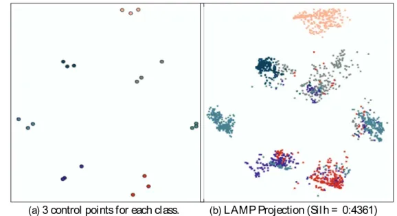
Figure26 – LAMP Projection (neighborhood in R2) using only 3 control points per class
(21 in total, against 137 needed to executePLP). . . 96
Figure27 – Description of an interactive system that uses LAMP to correlate different datasets that do not haveexplicit relation among instances. . . 96
Figure28 – Prototypesystem correlating imageand music.. . . 98
Figure29 – Application exploration of text documents. . . 100
Figure30 – Aggregate error view showing three detail levels: (a) a = 1;b = 1. (b) a = 5;b = 5. (c) a = 20;b = 20 pixels (seeSec. 4.4.2).. . . 109
Figure31 – False neighborsview (seeSec. 4.4.3).. . . 112
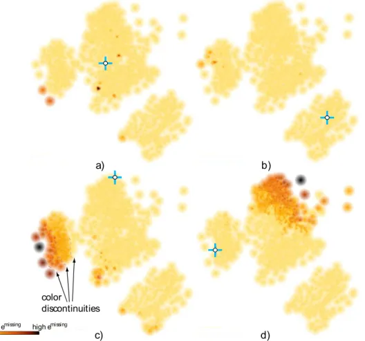
Figure32 – Missing neighbors view for four selected points (indicated by markers). See Sec. 4.4.4. . . 114
Figure33 – Missing neighbors finder view for four selected points. Selectionsareindi-cated by markers(see Sec. 4.4.5). . . 116
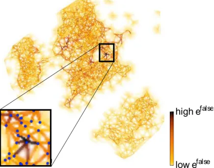
emissingG . Bottom images add edge bundles to indicate the most important
missing point-pairs. . . 120
Figure36 – Comparing projections. (a) LAMP(blue) and LSP(red) points. (b) Bundles show corresponding point groups in thetwo projections (seeSec. 4.4.7). . . 121
Figure37 – Global comparison of LAMP, LSP, PLMP, and Pekalskaprojections for the Segmentation dataset (see Sec. 4.5.4) . . . 127
Figure38 – LAMPalgorithm, Freefoto dataset, different neighbor percentagesper row (seealso Fig. 39). . . 128
Figure39 – LSPtechnique, Freefoto dataset, different numbers of control pointsper row (comparewith Fig. 38) . . . 130
Figure40 – Applications– LSP technique, Freefoto dataset, different numbersof neigh-bors. Bundles show most important missing neighneigh-bors. . . 131
Figure41 – Onealgorithm (LAMP), different datasets. Top row: falseneighbors. Bottom row: missing neighbors. . . 132
Figure42 – ISOMAPprojection, Corel dataset, finding missing group membersfor dif-ferent numbers of neighbors. . . 133
Figure43 – Shift between two LSPprojections, News dataset, for different numbersof force-directed iterations. . . 133
Figure44 – Scatterplot (a) and biplot (b) comparison. Green dots represent theinstances, or observations, and axesrepresent variables(GREENACRE, 2010). . . 142
Figure45 – Document dataset shown by a3D scatterplot.. . . 145
Figure46 – Adding curved biplot axesto the 3D projection in Fig. 45. . . 146
Figure47 – FBDR projection with labels and ticks. . . 147
Figure48 – Axislegends. Two clicks in the left view will align variables 0 and 6 with the screen x and y axesrespectively, leading to theright view. . . 148
Figure49 – Legend for viewpoint shown in Fig. 48 right.(a) Viewpoint sphere; (b) Matrix-plot view; (c) Transfer functions for color and luminance of the viewpoint sphere. . . 151
Figure50 – Selected viewpoint best showing scatterplot of variables 2 and 6. . . 152
Figure51 – Selecting thebest projection among threeDR techniques (FBDR, ISOMAP, LAMP) using biplot axes and axis legends. SeeSec. 5.4.1.. . . 155
Figure52 – Explaining, in terms of variables, the shapeof the 3D LAMPprojection of 10-variatemultifield simulation dataset (seeSec.5.4.2). . . 157
Figure53 – Visualization of 19-variate imagesegmentation dataset using 3D projections (a,b,d) and 2D projections (c,e). SeeSec. 5.4.3.. . . 160
Figure56 – Vertical rotation of shortest biplot axis(variable’3:inv’) and corresponding
aggregated error and falseneighbors views, synthetic dataset. . . 166
Figure57 – Best and worst viewpoints for the longest and shortest biplot axes, and corresponding false-neighbors and aggregated error views, real-world wine dataset. . . 168
Figure58 – Pipelineof theconstruction of our visual summarization. . . 178
Figure59 – Example of the visual outcome created by our technique. The skims with icons (1,3,4,7) represent events detected using themetadata. The other skims (2,5,6) were detected using only theaudio data. . . 181
Figure60 – Visualization constructed from audio highlightsonly. In thisrepresentation thematch is summarized according to the narrator’semotion and audience excitement.. . . 182
Figure61 – Visualization constructed from metadatainformation only.. . . 183
Figure62 – Visualization using audio and metadata information with different levels of detail. Themost important eventsarecaptured, someonly by themetadata (substitutions) and some only by theaudio (thegoal chances). . . 184
Figure63 – Dynamics of finalists in theknockout stageof the 2014 World Cup. . . 185
Figure64 – Visualization of dynamics of 2014 World Cup final match in six different languages. Different culturesdefine different views of a match. Our visual metaphor can beused to easily verify and analyzecultural aspects. . . 186
Figure65 – Statistics of users’ feedback gathered viausability questionnaires.. . . 189
Figure66 – Construction of a multidimensional dataset from avideo collection.. . . 192
Figure67 – Dataset design for scenario 1. . . 194
Figure68 – Scenario 1. (a) Point cloud. (b) Point cloud with 40% transparency. . . 194
Figure69 – Scenario 1. (a) points color coded by timestamp. (b) pointscolor coded by timestamp with 40% transparency. . . 195
Figure70 – Scenario 1. (a) points color coded by loudness. (b) color coded by loudness with 40% transparency. . . 196
Figure71 – Scenario 1. (a) points color coded by event types, with time and loudness axesoutlined. (b) pointscolor coded by events with 40% transparency. . . . 197
Figure72 – Scenario 1. (a) points color coded by match_id. (b) points color coded by match_id with 40% transparency. . . 197
Figure73 – Scenario 2 with 7 attributes per observation (fiveloudness, event_type, and match_id) . . . 199
Figure76 – Scenario 2. (a) pointscolor coded by timestamp. (b) pointscolor coded by timestamp with 40% transparency. . . 201
Figure77 – Scenario 2. (a) Pointscolored by match_id. Orange and bluepoints represent silent events. (b) Zoom-in on thehigh-loudnessoutliers. . . 202
Figure78 – Scenario 2. Dataprojected in 3D using fiveloudness dimensions. . . 202
Figure79 – Scenario 2. Dataprojected in 3D using five loudnessdimensions and times-tamp. Color codes timestimes-tamp. . . 203
Figure80 – Scenario 3 with 10 loudness and onetimestamp dimensions per observation, colored by event_type. . . 204
Figure81 – Scenario 3. (a) points projected using 10 loudnessdimensions. (b) sameplot, color coded by event_type, and rendered with 40% transparency. . . 205
Figure82 – Biplotsof Scenario 3 showing correlations of goalswith loudnessand vari-ability of theloudness patterns. . . 205
Table1 – Datasetsused in thecomparisons. . . 90
1 INTRODUCTION . . . 25
1.1 M ultidimensional data . . . 27
1.2 Visualizing multidimensional data . . . 27
1.3 M ultidimensional projections . . . 29
1.4 M ultimedia data . . . 29
1.5 Research questions . . . 31
2 RELATED WORK . . . 33
2.1 Introduction . . . 33
2.2 M ultidimensional data in context . . . 34
2.2.1 Taxonomies of data . . . 34
2.2.2 M ultidimensional data . . . 37
2.2.3 M ultidimensional data analysis challenges. . . 39
2.3 M ultidimensional Data Analysis. . . 41
2.3.1 Statistical Approaches . . . 43
2.3.2 Frequent Pattern M ining . . . 45
2.3.3 Classi cation . . . 46
2.3.4 Clustering . . . 47
2.4 M ultidimensional Data Visualization . . . 49
2.4.1 Axis-Based M ethods . . . 50
2.4.2 Space Filing Approaches . . . 58
2.4.3 M ultidimensional Projections . . . 60
2.4.4 Other Approaches . . . 69
2.5 Exploring M ultidimensional M ultimedia Data . . . 70
2.5.1 Video analysis steps. . . 71
2.5.2 Analysis and presentation of video content . . . 73
2.6 Conclusion . . . 79
3 LOCAL AFFINE M ULTIDIM ENSIONAL PROJECTION . . . 81
3.1 Introduction . . . 81
3.2 Technique Description . . . 84
3.2.1 A ne M apping Computation from Control Points . . . 85
3.4.1 Application 1: Correlating images and audio data . . . 96
3.4.2 Application 2: Document analysis . . . 99
3.5 Discussion. . . 100
3.6 Conclusion . . . 101
4 VISUAL ANALYSIS OF DIM ENSIONALITY REDUCTION QUAL-ITY FOR PARAM ETERIZED PROJECTIONS . . . 103
4.1 Introduction . . . 104
4.2 Related Work . . . 105
4.3 Explanation goals . . . 107
4.4 Proposed visualizations. . . 108
4.4.1 Distance preservation error . . . 108
4.4.2 Visualizing aggregated error . . . 108
4.4.3 Visualizing false neighbors . . . 111
4.4.4 Visualizing missing neighbors . . . 113
4.4.5 M issing neighbors nder . . . 115
4.4.6 Group analysis . . . 118
4.4.7 Comparing projections . . . 120
4.4.8 Proposed work ow . . . 122
4.4.8.1 Step 1 . . . 122
4.4.8.2 Step 2 . . . 122
4.4.8.3 Step 3 . . . 122
4.4.8.4 Step 4 . . . 123
4.5 Applications . . . 123
4.5.1 Description of Datasets . . . 123
4.5.2 Projection Techniques . . . 124
4.5.3 Projection parameters . . . 125
4.5.4 Overview comparison . . . 126
4.5.5 Parameter analysis . . . 126
4.6 Discussion. . . 134
4.7 Conclusions . . . 137
5 EXPLAINING 3D DIM ENSIONALITY REDUCTION PLOTS . . . 139
5.1 Introduction . . . 139
5.2 Related Work . . . 141
5.2.1 Explaining projections. . . 141
5.3 Explanatory visualizations . . . 145
5.4 Applications . . . 153
5.4.1 Wine dataset: Finding good DR projections . . . 154
5.4.2 M ulti eld dataset: Explaining projection shapes . . . 156
5.4.3 Segmentation dataset . . . 158
5.4.4 Software dataset: Finding meaningful clusters . . . 161
5.4.5 Axis alignment vs projection quality . . . 162
5.5 Discussion. . . 167
5.6 Conclusion . . . 170
6 THE SHAPE OF THE GAM E . . . 173
6.1 Introduction . . . 173
6.2 Related Work . . . 176
6.3 User-Centric Approach: Videoplayer-style Sports Video Sumarization177
6.3.1 Detection of audio highlights . . . 178
6.3.2 Detection of metadata highlights. . . 179
6.3.3 Constructing the visual representation . . . 179
6.4 User-Centric Approach: Results and Evaluation . . . 181
6.4.1 Datasets . . . 181
6.4.2 Visual exploration . . . 182
6.4.3 User Evaluation . . . 187
6.5 Data-Centric Approach: Sports Video Exploration with M ultidimen-sional Projections . . . 189
6.5.1 M ultidimensional Dataset Construction . . . 190
6.5.2 Visual exploration of the multidimensional multimedia data . . . 193
6.5.2.1 Scenario 1: Using low-dimensional scatterplots. . . 193
6.5.2.2 Scenario 2: Increasing the number of dimensions . . . 198
6.5.2.3 Scenario 3: Further increasing dimensionality . . . 203
6.6 Discussion. . . 206
6.7 Conclusions . . . 208
7 DISCUSSION AND CONCLUSIONS . . . 211
7.1 Future work. . . 215
CHAPTER
1
INTRODUCTION
In the last decade, the informational world has witnessed a major shift in structure, operation, and focus. Thisshift can be explained by the improvement and convergence of alarge and hybrid number of technical developments. Theadvent of faster, cheaper, and easier to deploy and usesensor technologies, such asvideo cameras, GPSdevices, medical body signal meters, proximity sensors, and laser scanners have made a rich and growing typeof information sources available to analysisand investigation. Theseparateadvent of cheap and fast storage space for data has madeit possibleto gather immenseamounts of dataof various types for thesamegoals of analysis and investigation. Thedevelopment of web-based communication technologies such asweb and cloud computing and software-as-a-servicehasdramatically increased both the range and bandwidth of data-processing functionality available to stakeholders ranging from large corporations to casual users.
Theabovedevelopments, which areoften known under thegeneric nameof ‘big data’, have opened many types of applications and investigations which were, until recent times, either thought to behardly possible, or elseconfined to therealm of anarrow set of technology-intensive organizations. Nowadays, big data applications such asfinding best-purchased products, most-relevant news articles and blog discussions, trends and outliers in shopping or travel of large groups of individuals, key topics in healthcare and lifestyle, and the evolution of stock portfolios under various market, social, and political factors, are available to both specialized corporate professionals and end users.
to the speed of change of data that isto be investigated, and is a by-product of the decreasing acquisition and storagecosts, and theincreasing simplicity and throughput of datasensors. As such, velocity can be seen as a multiplier for the volume factor, which in turn increases the challenges and needs for efficient, effective, and scalableanalysis and interpretations techniques and tools. Finally, variety refers to the increasing range of types of data that we can acquire, store, and wish to analyze. These rangefrom classical continuoussignal measurements, such astemperature, pressure, speed, velocity, altitude, and heartbeat (delivered by typical analogue-to-digital convertersand sensors) to text documents(mined from blogs, Twitter accounts, RSS feeds, and web-crawling tools); structured relational attributed graphs (mined e.g. from open-sourcesoftware repositories such asCVS, Subversion, and Git); and multimediadatainvolving collectionsof text, metadata, video, and audio streams(mined from surveillance cameras, live TV broadcasts, or web sitessuch as YouTube, Facebook, or Instagram).
Critical to an efficient and effectiveuse of big datais theavailability of equally efficient and effectivetechnologies to extract so-called actionable insight (KPMG International Coopera-tive.,2014;Mercer Marsh & McLellan,2014). Actionable insight can be generically defined as higher-level knowledge, extracted from ‘raw’ big datacollections, which enablesorganizationsto take actions that optimizeactivities such as sales, marketing, product optimization, and reducing cost and turnover times. Clearly, thethreecharacterizing aspectsof big data (volume, velocity, and variety) posevariouschallengesto extracting such actionableinsight in efficient and effective manners.
1.1 M ultidimensional data
The above-mentioned aspects of big data variety can be, technically, captured by the concept of a multidimensional dataset. Two elements are key to the description of such a dataset, as follows. First, an observation (also called sample, instance, or datapoint) comprises a set of measurements that pertain to the same entity. Examples are the video stream, audio stream, subtitles, textual descriptions, and metadatathat jointly describean uploaded video on YouTube or aTV broadcast of amovieor sportsmatch; or the files, folders, commit logs, change requests, quality metrics, and bug reports that jointly characterizea softwareproject stored in a softwarerepository such asSubversion or Git. Secondly, as implied by theabovedefinition, each observation is characterized by anumber of measurements(also called attributes, variables, or dimensions). In our examplesthesearethecharacteristics of thevideo, audio, text, and metadata that describe an uploaded video; or theprogramming language, source code, and number of type of reported bugs or filed changerequeststhat describea softwareproject.
In technical terms, multidimensional datasets can be modeled as a set of m observations, each onebeing regarded aspoint in an n-dimensional space. Whileelegant, generic, and compact, this datamodel creates several challenges from the perspectiveof extracting actionableinsights. Arguably the largest such challenge relatesto theinability of humansto depict spaceshaving more than 3 or, at best, 4 dimensions. Indeed, humans live and act in athree-dimensional space; assuch, understanding how databehavesin spaceshaving considerably moredimensionsishard, if not even impossible.
1.2 Visualizing multidimensional data
Oneimportant question to consider is why we would need to depict, or visualize, such high dimensional spaces. It can be argued that, after all, one could analyze high-dimensional datasets automatically, by running appropriatedatamining or pattern detection toolsand tech-niques, without the need to explicitly visualize the high-dimensional data. While this is true, the abovereasoning omits aso-called boostrapping problem: To beableto design an effective pattern detection or data mining algorithm, onehasto understand which patterns are relevant for thehigher-level application-dependent goalsat hand. Subsequently, in order to understand the relationships between such patterns and goals, one has to be able to visualize the patterns and their underlying ground-truth evidence to detect their characteristics which can, next, be encoded into automatic data mining or pattern searching algorithms. Separately, to be able to validate, fine tune, and improvetheaforementioned datamining algorithms, one hasto beable to correlatetheir behavior with theunderlying dataat hand and availableground-truth evidence. As such, at thecore – or better said, at theinception – of thedesign of datamining algorithms for multidimensional datasets is theability of humans to directly investigatesuch datasets.
fields of science. At a high level data visualization is concerned with the creation of 2D and 3D depictions of all kinds and types of data collections, or datasets, with a focus on datasets which are naturally represented by spatial shapes, such as 2D images, 3D volumetric scans, and theresults of 2D and 3D measurementsand simulationsof physical processessuch as heat dissipation, mechanical deformation, or fluid flow (SCHROEDER; MARTIN; LORENSEN,
2006; TELEA,2014). At a more specific level, information visualization is concerned with thecreation of 2D and 3D depictions of datasets which do not have anatural representation in physical spaceand/or whosedimensionality is far higher than three, such as graphs, networks, relational data tables, or our multidimensional datasets consisting of multimedia or software measurementsintroduced earlier (WARD; GRINSTEIN; KEIM,2010;MUNZNER,2015). At an even morespecific level, visual analytics refines both dataand information visualization by adding customized workflows, typically based on interactivetechniques, to analyzethedepicted data with theaims of forming, (dis)proving, and refining hypotheses – aprocess globally known under the name of ‘sensemaking’ (THOMAS; COOK,2005;KEIM et al.,2010). At aglobal level, all above-mentioned visualization techniqueshave thesameaims– making theinvisible (data) visible, and supporting activities such as confirming the known and discovering the unknown (in thedata).
Central to the design (and success) of a data visualization application is the ability of mapping the essential aspects of the dataset(s) under study to recognizable 2D and/or 3D shapes, colors, and patterns. If such patterns arecarefully chosen, users can (a) easily recognize them, even in the presence of considerable noise and variability, and (b) next map them back to phenomenapresent in theoriginal data, by aprocessknown as‘inversemapping’ (TELEA,
2014). Much work hasbeen dedicated to thestudy of which so-called visual encodings (of data) best servespecific data analysistasksfor specific kindsof datasets(TUFTE,2001). Thiswork hasgiven riseto awealth of specific methods and visualization subfieldssuch as scalar, vector, and tensor visualization (SCHROEDER; MARTIN; LORENSEN,2006); graph and network drawing (Di Battistaet al.,1999); and information visualization (MUNZNER,2015).
1.3 M ultidimensional projections
A different solution to the visualization of multidimensional data is proposed by the so-called multidimensional projection methods. These methods are also known under various other names, such as dimensionality reduction and multidimensional scaling. In a nutshell, such methodstakea dataset having hundreds or even thousandsof dimensions per observation, and construct a new dataset having the same number of observations but only two or three dimensions. Key to theworking of projection methods is their aim to preservetheso-called data structure in the resulting low-dimensional space. This takes the form or e.g. preserving distances between pairsof observations or preserving the neighborhoods of observations. If such goals can beachieved efficiently and effectively, theuserscan employ the resulting low-dimensional projection asa ‘proxy’ to study the invisiblehigh-dimensional spaces. For instance, tasks such asfinding outliers, groupsof highly-related observations, correlated dimensions, trendsin the dimensions’ values can all be performed on the low-dimensional space, which is typically displayed as acolor-coded scatterplot of observations.
In the last decade, awealth of multidimensional projection methods has been developed. Current methods, and their corresponding implementations, are very successful in computing projectionsof datasetshaving a largenumber of observations, each having tensdimensionsor more, at near-interactive rates, and with a good preservation of relevant quality metrics such as distancesor neighborhoods of observations. Additionally, most such methodscan bereadily used by developers and end usersin alargely black-box fashion, i.e., without having to know or understand theintricaciesof their implementations. However, projection-based visualizations are significantly hampered by their abstract nature: In thetypical case, they deliver a2D scatterplot where each observation isencoded as apoint. Whilethis allows oneto tell whether thedataset under study contains outliers, or groups of related observations, it doesnot tell users why such structuresappear in the data. For instance, we can easily locate an outlier observation in a 2D scatterplot created by amultidimensional projection, but wedo not know which attribute(s) of the respectiveobservation makethat point so different from therest. Similarly, wemay beable to easily see that aset of observationsconsistsof threegroups of well-separated points, but we do not know which attribute(s) make the points in a group belong together. Altogether, these aspectssignificantly decreasetheusability and acceptability of projection techniques for large classesof non-specialist userssuch as businessand market analysts, let alonecasual end users.
1.4 M ultimedia data
∙ Prevalence: Multimediadataareof increasing availability and importance in all contexts wherebig dataplaysarole. It isavailable at low or even zero costs, being provided at high volume, velocity, and variety on social media channelssuch asYouTube, Facebook, the world wideweb, or morespecialized movieor TV collections;
∙ Complexity: Multimediadataare by excellencehighly variate, in the sense of containing a (large) range of attributesof different types. These include video and imagedescriptors suchase.g. SIFT andSURFfeatures(LOWE,1999), imagemoments(PROKOP; REEVES,
1992), color and brightnesshistograms(SEZGIN; SANKUR,2004), and featuresextracted from face recognition (ZHAO et al.,2003); audio descriptorssuch aspitch, volume, and speech-to-text descriptors (AYADI; KAMEL; KARRAY,2011); and metadata descriptors such askeywords extracted from provided subtitles, user comments, or categorical ratings and classifications of videos. Altogether, the above provide a rich high-dimensional collection of attributesof various types that characterizes multimedia data – and therefore an explicit challengeto multidimensional datavisualization;
∙ Reach: Multimediadata hasaclearly wide reach to extremely various typesof users being interested in highly different goals and having highly different skills and expectations. These range from professional surveillance analysts and coaches of sports teams, who have thetraining and timerequired to interpret highly detailed and sophisticated analyses, to casual end userssuch asteenagers browsing video collectionsor sportsfanswatching seriesof soccer matches. While the input dataisidentical in all thesecases, the techniques required to satisfy theneeds of these user groups clearly haveto beof different types.
1.5 Research questions
Having introduced the generic challengesof visual exploration of multidimensional data, and themorespecific challengesof exploring multimediadata, wecan now formulateour two key research questions:
Question 1: How can we design ways to interactively exploremultidimensional projections that convey to users insights on the semantics of the patterns perceived in the projection space, in termsof aspects of thehigh-dimensional data?
Question 2: How can wedesign ways to interactively explore multidimensional data extracted from multimedia datasets so as to support a wide range of tasks for different types of users ranging fromprofessionalsto casual users?
Theabovetwoquestionsarerelated at several levels. First, effectiveand efficient solutions to Question 1 may servethebasisof designing effectiveand efficient solutions(tools) that satisfy thegoalsposed by theusers listed under Question 2. Secondly, specific goalsand requirements of theusers under Question 2 can form test scenarios to validate, or show thelimitations of, the methodsdesigned to solveQuestion 1. Thirdly, multimediadataformsby itself arich, complex, and easily available corpus of information that serves to test methods designed to solve both Questions1 and 2.
In linewith the abovetwo coupled research questions, the structure of thisthesisisas follows.
In Chapter2, wediscussrelated work in theareasof (visual) analysisof multidimensional dataand themorespecific analysis goalsof multimediadata.
Chapter3explores the use of projection techniques for the visual depiction of large multidimensional datasets. To thisend, wepresent anovel multidimensional projection technique which competes favorably, or even exceeds, desirable features of state-of-the-art projection techniques such as generality, computational scalability, precision in preserving inter-point distances, algorithmic robustness, and – last but not least – the ability to control the shape of theresulting projection by interactiveplacement of asmall number of selected datapoints. We demonstrate the application of our proposed technique by two use cases involving the joint exploration of audio-and-video multimediacollections and the exploration of collections of text documents.
high-dimensional datastructure, areaffected by parametersof the projection techniques being used. Weintroduce several metrics to quantify the quality and variability of a projection, and show how such metrics can be visually depicted in intuitiveand easily usable ways. By this, we makethefirst step into explaining multidimensional projections to their typical end users. We demonstrate our proposed techniques for a widerange of multidimensional datasets and existing projection techniques.
Chapter5addresses the task of explaining 3D multidimensional projections in terms of the attributes, or dimensions, of the projected high-dimensional datasets. Specifically, we present a number of interactive exploration and explanation mechanismsthat inform userson the meaning of the visible data structures in a 3D projection in terms of the underlying high-dimensional variables, and let usersbrowsethe space of possibleviewpoints of a3D projection to find viewpoints from which specific variable-groups can be best analyzed. This makes the second step in our quest towards explaining multidimensional projections to their typical end users. We demonstrate our proposed techniques for a range of multidimensional datasets and projection techniques, and also show theadded-valueof using 3D projections, annotated by our explanatory mechanisms, ascompared to thebetter-known 2D projections.
CHAPTER
2
RELATED WORK
Abstract: Multidimensional datasets pose numerous challenges in terms of efficiently and ef-fectively analyzing them to extract useful and usable insights for problem solving. Several of these challenges stem from the difficulty of capturing and explaining patterns caused by the values of multiple attributes sampled over many observations, and from thefact that it is hard for humansto form an intuitivedepiction of high-dimensional dataspaces. In thischapter wepresent a taxonomy of multidimensional data and overview the different analysis and visualization methodsproposed for exploring such data, with a focus on multidimensional projection methods. Separately, we overview existing methods for the visual exploration of large multimedia data collections, with afocus on the multidimensional natureof theinvolved data. We conclude that multidimensional projections can beefficient and effectivetechniquesto usein the construction of visual exploration tools for multimedia datasets.
2.1 Introduction
2.2 M ultidimensional data in context
Beforestarting theanalysis process, it is essential to haveagood understanding of the kind of datathat isbeing analyzed. Therefore, thefirst step in theanalysis of dataisto get clarity about the data’s intrinsic nature, meaning, structure, and type. Characterizing the nature and meaning of databy, for instance, capturing the variability of theseaspects into aclassification or taxonomy, is avery challenging endeavor (MUNZNER,2015). Indeed, the samedataset can be regarded from multipleperspectives, depending on thetype of questionsor analysisthat wewant to address. Assuch, whilehaving agood understanding of datanatureand meaning is definitely important for solving a concrete data-related problem, there are few universal guidelines to be applied in this process. In contrast, characterizing the data structure and type by means of taxonomies is auseful and effectiveinstrument to guideresearcherstowardsspecific classes of analysisand visualization techniquessuited for their concretedatasets(SCHROEDER; MARTIN; LORENSEN,2006;SHNEIDERMAN,1996).
2.2.1 Taxonomies of data
Several taxonomies have been proposed for classifying data in terms of structure and type. With respect to the visual exploration (or visualization) options that such taxonomies associate to different datasets, we note the classification of data in terms of spatial vs non-spatial (MUNZNER,2015): Spatial data is seen as the value of a function f whose domain D is a (typically compact) subset of R2or R3. Data values, or samples f (xi), are recorded
at sample points xi ∈D. Depending on the distribution of the sample points xi over D, we
distinguish between different types of dataset sampling strategies, or grids, such asuniform or regular, rectilinear, structured, and unstructured (TELEA,2014). Different types of gridstrade off implementation simplicity and low storage costs against flexibility to place sample points at desired locations over D to achieve an optimal capture of the shape of f with a minimal number of samples. Non-spatial dataisseen asthevalueof afunction f whosedomain D isnot a (compact) subset of a continuous spacesuch asR2or R3. Implementation-wise, non-spatial data
also consistsof anumber of data values f (xi) recorded at anumber of points xi∈D. However,
in contrast to spatial data, the points xi can not beregarded as asampling of acontinuous space–
thereis simply no databetween thepointsxi. Assuch, thepointsxi wheredatais recorded are
typically called datapointsor observations, rather than samplepoints.
A further refinement of spatial data taxonomy regards thetypeof values of thefunction f , or therangeRof f . Such values f (xi) are also called dataattributes. Attributes aretypically
classified according to theoperations that R permits. In decreasing order of sophistication, the following attributetypesarecommonly identified (MUNZNER,2015;TELEA,2014;HANSEN; JOHNSON,2005):1
1 Attribute taxonomies bear an interesting, though not further exploited similarity (to our knowledge), with
∙ quantitative: Quantitativeattributes, also called continuousor ratio attributes, are defined over ranges R that allow operations such as addition, subtraction, and multiplication by a real number. Most commonly, such attributes are real values, i.e. R⊂ R. Spatial datahaving quantitativeattributesisfrequently met in thecontext of so-called scientific visualization (scivis) datasets. Exampleshereof areheight fields, grayscaleor color images, CT or MRI scans, and 2D and 3D vector fieldscreated by computational flow dynamic (CFD) simulations(HANSEN; JOHNSON,2005). A key characteristic of spatial datasets having quantitative attributes is that these datasets naturally allow interpolation of data values. In detail, for any point x located in the dataset domain D, we can estimate the interpolated valueof the function f (x) asafunction of thedatavalues, or samples, f (xi)
at samplepointsxi∈D located at points xi closeto x. Interpolation isacrucial capability
for supporting operations such as reconstruction (re-creating a piecewise continuous, version of f over D from the samples f (xi)), resampling, and smoothing. In turn, such
operations addresstaskssuch as datasimplification and aggregation, which support the visual exploration of very largedatasets.
∙ integral: Integral attributes, sometimes also called discrete attributes, are defined over rangesRthat allow operationssuch asaddition and subtraction, but not multiplication by a real number. Most commonly, such attributes are domains R⊂Z. Non-spatial datahaving integral attributes is frequently met in thecontext of so-called information visualization (infovis) datasets. Examples hereof are tableswhose cellsrepresent counts, like number of personsin a census (MUNZNER,2015). In contrast to quantitative datasets, integral datasets do not (formally speaking) admit interpolation. Indeed, even if this is technically possible, interpolation of integral values would typically createreal values, which thus are outside of thedomain R⊂Z.
∙ ordinal: Ordinal attributesaredefined over rangesRthat allow operationssuch asordering, i.e. definetherelations < , > , and = . Examplesof such attributes are ordered sequences of ranks of observations, such as Likert 5-point scales used to assess the quality of aproduct, e.g. R = { very poor, poor, neutral, good, very good} , or scales used to quantify the acceptancelikelihood of a scientific publication submitted for review, e.g. R= { definitely reject, possibly reject, borderline, possibly accept, definitely accept} . Ordinal attributes typically do not allow interpolation.
∙ categorical: Categorical, or nominal, attributes are defined over any set R. The only operation allowed by such attributes is, thus, checking for identity or equality of two elements. Examples of such attributes are types of elements, such as gender (male or female) or vehicle type (car, plane, train, or ship). Categorical attributes can be further organized in hierarchiesor taxonomies, based on theperceived similarity of datavalues.
When thisispossible, categorical attributesalso allow computing thedistance, or similarity, between data values. As distance is an integral or quantitative value type, this allows mapping categorical attributes to data types that allow more powerful operations, thus support awider rangeof analyses and explorations.
∙ text: Text attributes are defined over the set of all possible text strings generated by a given letter alphabet, or over a more restricted set of phrases or words captured by agiven dictionary. Formally speaking, text attributes can beseen aseither ordinal (sincestrings admit ordering e.g. in terms of lexicographic order) or categorical (since we can easily tell when two strings are identical or not). Moreover, distances can becomputed over text attributes, e.g. in termsof theLevenshtein metric (LEVENSHTEIN,1966). However, in many practical applications, text attributes attempt to capture moreinvolved information than what string comparison, lexicographic order, and Levenshtein distances can model. For instance, typical text analysisand mining applications need to avail of morecomplex metrics that capture the semantic similarity of text fragments. When such metrics can be computed from text attributes, we can reducesuch attributes to (sets of) quantitative, ordinal, and categorical derived attributes.
∙ relational: Relational attributes are defined over sets of data points in D. Their range R is thus the set of all possible subsets of elements in D, or the power set of D. In many fields, such attributes are known as graphs or networks. Here, the nodes represent data pointsin D, and edges capture the relations between these data points which are part of R. Graphscan befurther specialized into directed and undirected, cyclic or acyclic, and trees or hierarchies. Graphs are ubiquitous in many information visualization subfields, such as software visualization (softvis), where they capture the structureand dependencies of software systems (DIEHL,2010); and geographical visualization (geovis) (DYKES; MACEACHREN; KRAAK,2005), where they capture the structure of road or similar transportation networks. Thevisual exploration of graphsformsthefocusof thespecialized subfieldsof graph visualization and graph drawing (Di Battista et al.,1999). Relational attributes form aseparate case as compared to the earlier discussed attributetypes (quanti-tative, integral, ordinal, categorical, and text): Indeed, whilethese earlier attributetypes describea property solely associated to a datapoint or observation xi, relational attributes
describeproperties associated to sets of (minimally two) such datapoints { xi} .
1999;HERMAN; CON; MARSHALL,2000). Multidimensional datasets including relational attributes forms asub-field of interest of graph visualization, which proposes specific methods that aim to emphasizetherelational natureof the data and also visually encode several attributes per node and/or edge (DIEHL; TELEA,2013;WATTENBERG,2006;PRETORIUS; WIJK,
2006). Overall, the nesting of attribute typesindicated above allows using visual exploration and analysis methods defined for theless ‘powerful’ attributetypesto be applied to more powerful attributetypes, but not conversely.
Datasetshavingquantitativeattributesdefined at datapointssampled over spatial domains aresometimesalso called continuousdatasets, asthey allow interpolation, asexplained earlier. In contrast, datasetshaving (1) quantitativeattributesdefined over non-spatial domains, and also (2) datasetshaving any attributes besides quantitativeones, aresometimescalled discrete datasets, as they do not allow interpolation, either because of the lack of a distance metric between samplepoints(case (1) above), or becauseof the lack of necessary operations for interpolation such as multiplication with a real-valued number (case(2) above). To strengthen thedifference between continuous and discrete datasets, the latter aresometimes also called inherently discrete datasets(TELEA,2014). This underlinesthedifferencebetween adiscretedataset containing quantitative attributes, obtained by the sampling of a continuoussignal over a spatial domain, which naturally admits interpolation to apiecewise-continuousresult; and adiscretedataset of types (1) or (2), which does not admit interpolation, for thereasons outlined above.
Other taxonomiesof, or related to, data used in visualization have been proposed. For instance, Shneiderman proposes ataxonomy of visual exploration tasks by the datatypebeing involved in the respective task (SHNEIDERMAN, 1996). Seven data types are recognized: one-, two-, and three-dimensional datasets (thedimension herebeing roughly equivalent to the dimensionality of our set D introduced at the beginning of Sec.2.2.1); temporal datasets; trees; networks; and multidimensional data. However, thetaxonomy isnot further refined in depth up to alevel whereone can decideon visualization methods best suited for a given datatype. Also, multidimensional datais discussed only briefly. Chan proposes ataxonomy of visualization tech-niques for multivariatedata, along thelinesproposed by Keim and Kriegel (KEIM; KRIEGEL,
1996;KEIM,1997) in geometric, icon-based, pixel-oriented, hierarchical, graph-based and hy-brid techniques. However, this work does not outline an explicit taxonomy for multidimensional dataitself.
2.2.2 M ultidimensional data
Following the dataset model presented above (a function f : D → R), we can further distinguish between datasets which record a single-valued attributeper point and datasets which record multi-valued attributes per point. Examples of the first category, for spatial datasets, arescalar-valued datasets or scalar fields (R⊂R); 2D and 3D vector-valued datasets or vector fields (R⊂R2and R⊂ R3, respectively); and color images (R⊂ R3
idea, weobtain thecaseof multidimensional datasets whereR⊂Rn, whereeach datapoint has
n real-valued attributes. Examples hereof include numerical simulations where, at each data point, one records several physical quantities, such as velocity, pressure, temperature, and matter density.
Multidimensional datasets arealso ubiquitous in thecaseof non-spatial datasets. Prob-ably the best known example of such datasets are data tables. In a data table, we can see each row as a data point or observation xi. Each column of the table, thus, records the
val-ues of adifferent attribute over all observations. Hence, a table having m rowsand n columns recordsmobservationseach having n attributes, or an n-dimensional attribute(SHNEIDERMAN,
1996). In our functional notation introduced in Sec.2.2.1, such adatatablecan bethought as a function f : { 1;:::;m} → Rn, whereRisthedomain of definition of thevaluesof adatatablecell.
Variabletypes: Within therealm of multidimensional data, wecan distinguish two subcases, based on the existing dependency relations between attributes. Consider, for instance, a m-column data table where the last k < m m-columns represent the output of a simulation and the first m− k columnsrepresent thecorresponding simulation inputs. Wesay, in other words, that the last k columns depend on the first m− k columns. This allows classifying attributes, also called variables, into dependent and independent ones. Related to this, traditional statistics refers to attributes as variates, with their complexity associated with univariate, bivariate and multivariatedata, as afunction on thenumber k of dependent variables(HAIR et al.,2006). In thevisualization field, however, theterms ‘multidimensional’ and ’multivariate’ are often used interchangeably to denoteadataset where, for each datapoint or observation, wehavemore than oneattributevalue(thus, m> 1). For instance, someauthorsrelatetheabovetwo termsto the dependent vs independent natureof attributes, by using the term ‘multivariate’ when we have several dependent variables(k > 1) and ‘multidimensional’ when wehaveseveral independent variables (m− k > 1) (SANTOS; BRODLIE,2004). In contrast, other authors use the terms ‘multivariate’ (TELEA,2014), ‘multidimensional’ (KEIM,2002;SHNEIDERMAN,1996), or ‘multivariables’ (SANTOS; BRODLIE,2004) to refer to both independent and dependent
vari-ables. As aconsequenceof theaboveterminology, values of observations are also known under different names, such as data-point values, observation values, dimensions, attributes, variables, and features(MUNZNER,2015).
or observation is described by several scalar-valued attributes. Vector fields, in contrast, are a subset of vector-valued data, where, at each point or observation x∈Rin thedomain of definition, wecan defineaso-called tangent vector, i.e. avector that leadsusfrom x to another point located inside R. Examples of vector fields are color images (m = 3 scalar attributes, R⊂ R2) and
flow fields in three-dimensional computational flow dynamics (m= 3, R⊂R3). In contrast, a
general datatablehaving threecolumnsrepresents, technically speaking, thesamedataset (m= 3 attributes), but isnot avector field, sincethereisno domain Rhaving theaforementioned tangent vector property. A separate distinction between vector-valued dataand multivariate data refers to theinterpretation of thedataattributes. In vector-valued datasets, them attributesrecorded per observation may be related, but can be studied equally well independently on each other, like in the case of a data table recording the age, salary, and profession of a set of individuals. In contrast, in a multivariatedataset, the samemattributes areintrinsically related, so they should be (normally) studied together, likein thecase of an image recording thered, green, and blue componentsof each pixel.
As the focus of the work in this thesis concerns the analysis of data having multiple attribute values per observation (m > 1), but without making a specific distinction between dependent and independent variables, and without making any assumptions on the nature of thedomain of definition R of thesevariables, nor on theexisting and/or important relationships between individual attributes, theterminology wehave adopted is that of multidimensional data. This terminology is themorecommon onebeing found in information visualization literature, and it also reflects the names of several important visualization methods in our context (e.g., multidimensional projections). Separately, wewill next use thetermsvariables, attributes, and dimensions to refer to the values of observations, in linewith thebest suited term for the specific discussion context. Finally, when mentioning multidimensional data, our focuswill implicitly be on datasetshaving ahigh number of dimensionsper observation (tens up to thousands), rather than multidimensional datahaving a low number of dimensions, such as2D or 3D vector fields.
2.2.3 M ultidimensional data analysis challenges
Multidimensional dataoffers someof thelargest challengesto data mining, dataanalysis, and dataexploration, and is one of thetopicsof theso-called ‘grand challenges’ in information visualization and visual analytics (THOMAS; COOK,2005;KEIM et al.,2010). Thedifficulty of understanding (phenomena described by) multidimensional datais caused by several aspects:
asinglereal-valued variable f : R → R. Analyzing such afunction isrelatively easy, by using e.g. itsfirst and second-order derivativesto e.g. reason about its rate of changeand local extrema. In contrast, consider a function of ten real-valued variables f : R10→ R.
Analyzing such a function is considerably more complex, as there exist a much larger family of first and second-order partial derivatives.
∙ Abstract nature: Low-dimensional data such as 2D or 3D fields can be relatively easy understood by directly plotting the recorded values by using a rangeof classical visual-ization methods. For discrete datasets, these methods include scatterplots, height plots, bar charts, and histograms. For data admitting interpolation, other specialized methods exist, such as height plots, contour plots, streamlines, and hedgehog plots. Such methods are well known and well proven in the domain of scientific visualization (HANSEN; JOHNSON,2005;SCHROEDER; MARTIN; LORENSEN,2006;TELEA,2014). The key advantageof being able to directly plot low-dimensional data is that we can identify and reason about complex patternsby simply seeing them, and without needing potentially complex waysto automatically find and quantify them. For instance, it isrelatively easy for moderately-trained end users to spot the presence of vortices, sources, and sinks in 2D vector fields, even though automatic detection thereof isstill acomplex problem (KOLAR,
2007). In contrast, humansdo not haveadirect intuition of spacesof dimensionality higher than 3. As such, directly understanding high-dimensional datasets is considerably harder, as wehaveto somehow project them into thelow-dimensional (2D or 3D) spacesweare ableto seeand reason about.
∙ Discontinuousnature: Many multidimensional datasetsinvolvedataattributeswhichdo not (easily) admit interpolation. Ordinal and categorical attributes areprimeexamples hereof (Sec.2.2.1). Assuch, wecannot createsmooth, continuous, representationsof such datasets with thesame easeas wecan, for example, when dealing with quantitative attributes. This creates several challenges even for low-dimensional data. For example, consider a 3D scalar volume, such as aCT or MRI scan. Astheunderlying datafrom which this dataset was constructed (viasampling) is inherently continuous, we can usevarious interpolation techniques to create smooth, continuous, and easy to understand representationsthereof, such as volume-rendered visualizations (LICHTENBELT; CRANE; NAQVI,1998). In contrast, consider adatatablehaving three columns, all containing quantitativeattributes. We can visualize these data by means of a 3D scatterplot, which would generate a 3D point cloud. As there is no continuity (no information is plotted between the points), understanding such a point cloud ismuch harder than understanding theearlier 3D scalar volumefield.
dataset having onemillion samplepoints which record the samples of afunction f : R → R We can easily construct a view of such a dataset, e.g. in terms of a classical graph y = f (x), and explorethegraph by classical interaction techniques such as zooming and panning. In contrast, consider a 100-dimensional scalar dataset having 10000 sample points. While the amount of data are the sameasfor thefirst case, understanding this100-dimensional dataset isconsiderably harder. This is due mainly to the fact that, for this dataset, understanding a single data point meansreasoning about 100 values. In contrast, understanding a singledatapoint for theearlier 1D dataset involves understanding a single data value. The problem compounds itself when aiming to perform morecomplex analyses. For instance, finding thedistance between two data points involves, in the 1D scalar dataset case, comparing two data values; doing the same for the 100-dimensional dataset involves comparing 200 data values. This inherent problem caused by the number of attributesin multidimensional data issometimesreferred to asthe ‘curseof dimensionality’ (BELLMAN,1961;YI et al.,2005). Such understanding challenges involving high-dimensional datasets will be discussed in more detail in Sec.2.4in the context of visual dataexploration.
2.3 M ultidimensional Data Analysis
Given our focus on multidimensional data exploration, we next discuss methods and techniques aimed to support various types of analyses of such data. These techniques will form thebasis of thevisual exploration, or visualization, techniques for multidimensional data discussed next in Sec.2.4.
To unify thediscussion, wefirst introduceseveral notationsto refinethedescription, first introduced in Sec.2.2, of amultidimensional dataset. Wemodel such adataset asacollection D = { xi} of mdatapoints, or observationsxi, which areidentified by their index of ID 1 ≤ i ≤ m.
Each observation xi is a tuple xi = (x1i;:::;xni) of n attributes, or variables xij, 1 ≤ j ≤ n. The
number of variables n givesthedimensionality of D . We denote thevalues of the jthvariable
over all mpointsof D by thevector xj= (xj
1;:::;xmj ). Wefurther assumethat all elementsof any
xj belong to thesamedomain – or, in other words, that all n variableshave well-defined types.
Thesecan be, formally speaking, any of thetypesdiscussed earlier in Sec.2.2.1, i.e., quantitative, integral, ordinal, categorical, text, or relations. However, in our discussion (and theremainder of this thesis) wewill focus mainly on quantitative, integral, ordinal, and categorical attributes, as thesetypeslargely cover most typical applicationsinvolving multidimensional data. In particular, we do not assume that all attributes are only of the quantitative type, which admits the useful property of interpolation (Sec. 2.2.1). Separately, wedo not assumethat different variables have the sameattributetypes.
daily, either by privatecompanies, governments or even casual users, it is evident that weneed mechanismsand toolsto extract useful information from thisdataexplosion. In thiscontext, data mining, also known as Knowledge Discovery from Data, or KDD for short, isa rapidly growing research-and-applications domain. Theaims of KDD techniquesand tools arethediscovery of useful information in largeand complex datasets; the identification of novel and useful patterns that – without the application of KDD methods – would otherwise remain unknown; and the creation of prediction models to discover trendsin those datasets (PANG-NING et al.,2006). KDD techniques and tools span the entire spectrum of user involvement, ranging from fully automatic to user-supervised techniques and finally ending with techniques where the data exploration is controlled and driven in detail by theuser.
Datamining processesaretypically integrated in pipelines, or setsof cascaded operations, where theraw input data isgradually transformed to yield the extracted knowledge of interest at theend. Such preprocessing operations havebeen classified by Han et al. in thefollowing four categories (HAN; KAMBER; PEI,2011):
∙ Data cleaning aims to remove noise and inconsistencies present in the input data. In our terminology, this step aims to make the dataset D a faithful representation of the underlying phenomenon it triesto sample;
∙ Data integration merges data from multiple acquisition sources into a coherent dataset. Thisinvolves, for instance, joining variables xj acquired from different sources and/or by
different sampling processes to createthefinal set of dimensions that characterizes D . ∙ Data transformation transforms or consolidates data to support the application of data
mining techniques. Transformation involves, for instance, filtering and resampling of the various dimensionsxj.
∙ Data reduction reduces data size. This can take the form of reducing the number of observations xi or the number of dimensions xj. In both cases, data reduction aims to
increasethescalability of theKDD methodswhich are subsequently applied to theinput dataset D .
Asalready implied by thepipelineconcept mentioned above, thefour typesof datapreprocessing operations are not mutually exclusive, but can be applied jointly in the analysis of specific datasets. Separately, wenotethesimilarity of such dataprocessing pipelineswith thewell-known concept of visualization pipelines used to describedata visualization processes (SCHROEDER; MARTIN; LORENSEN,2006;TELEA,2014): The transformation of datafrom itsraw input form into the high-level results, or insights, delivered by the KDD pipeline, is similar to the effect of thedataimporting, filtering, and mapping steps of thevisualization pipeline.
reduced by either reducing the number of dimensionsxj or thenumber of observationsxi. The
first typeof technique– dimensionality reduction – will beextensively discussed in Section2.4, given itsstrong integration with datavisualization techniques. Thesecond typeof technique– dataaggregation – is discussed next.
In our context, we denote by data aggregation the (wide) spectrum of techniques that attempt to reduce the number of observations xi present in a dataset D , to create a reduced
dataset D′ which preserves the essence of the phenomena of interest captured by the original
dataset D (PANG-NING et al.,2006). In thissense, dataaggregation can beseen asaprocess of eliminating observations by finding similarly-valued observations xi∈D and next replacing
subsets of such similar-valueobservations{ xi} by a singlesubsample, or representativex′i. This
way, undesirableaspects captured by D , such as outliers or acquisition noise, will beeliminated. Separately, the resulting aggregated dataset D′ will now capture only the stable,
statistically-relevant, structurespresent in thephenomenon sampled by theinput dataset D . A final advantage of dataaggregation techniquesisthat they reducethe amount of data that needsto be treated – either by subsequent data-analysis techniques or otherwise by data visualization techniques – and thereby increase the scalability of KDD pipelines. However, data aggregation techniques comewith an important (implicit) challenge: By eliminating observations, such techniquesmay eliminate actual features of interest from the underlying phenomenon. A well-known instance of this problem is theelimination of small-scale variationsin thedata, which can beseen as either noiseor small-scaledetail, depending on their context.
Many data mining techniques have proven to be very successful in the context of analyzing multidimensional datasets. Following Wang et al. (WANG; YANG,2010) and Pang et al. (PANG-NING et al.,2006), we identify four types of such techniques: frequent pattern mining, clustering, classification, and statistical analysis. These four types of techniques are discussed next.
2.3.1 Statistical Approaches
Statistical approaches arearguably the oldest and simplest typesof dataanalysis tech-niques for multidimensional datasets. Many such techtech-niques essentially aim to reducethesize and/or complexity of a given input dataset D to a compact representation entailing a few fig-ures that characterize the involved dimensions xj. In this respect, several techniques can be
applied (PANG-NING et al.,2006). Meansor medianscan be calculated for each dimension xj
if one wants to characterize each such dimension by a single scalar value representing ameasure of thelikelihood of theobservations xi. For instance, themean, or centroid, of theobservations
xi∈D ⊂Rnis given by
X = (x1;:::;xn)∈Rn; (2.1)
where xj is the mean of dimension xj of D . Besides the mean xj of a dimension xj, other