ACPD
15, 35547–35589, 2015DMS in the Canadian Arctic
E. L. Mungall et al.
Title Page
Abstract Introduction
Conclusions References
Tables Figures
◭ ◮
◭ ◮
Back Close
Full Screen / Esc
Printer-friendly Version Interactive Discussion
Discussion
P
a
per
|
Discussion
P
a
per
|
Discussion
P
a
per
|
Discussion
P
a
per
|
Atmos. Chem. Phys. Discuss., 15, 35547–35589, 2015 www.atmos-chem-phys-discuss.net/15/35547/2015/ doi:10.5194/acpd-15-35547-2015
© Author(s) 2015. CC Attribution 3.0 License.
This discussion paper is/has been under review for the journal Atmospheric Chemistry and Physics (ACP). Please refer to the corresponding final paper in ACP if available.
Summertime sources of dimethyl sulfide
in the Canadian Arctic Archipelago and
Ba
ffi
n Bay
E. L. Mungall1, B. Croft2, M. Lizotte3, J. L. Thomas4, J. G. Murphy1,
M. Levasseur3, R. V. Martin2, J. J. B. Wentzell5, J. Liggio5, and J. P. D. Abbatt1
1
Department of Chemistry, University of Toronto, Toronto, Canada 2
Department of Physics and Atmospheric Science, Dalhousie University, Halifax, Canada 3
Québec-Océan, Department of Biology, Université Laval, Québec, Canada 4
Sorbonne Universités, UPMC Univ. Paris 06, Université Versailles St-Quentin, CNRS/INSU, LATMOS-IPSL, Paris, France
5
Air Quality Processes Research Section, Environment Canada, Toronto, Ontario, Canada
Received: 1 December 2015 – Accepted: 4 December 2015 – Published: 16 December 2015
Correspondence to: J. Abbatt ([email protected])
ACPD
15, 35547–35589, 2015DMS in the Canadian Arctic
E. L. Mungall et al.
Title Page
Abstract Introduction
Conclusions References
Tables Figures
◭ ◮
◭ ◮
Back Close
Full Screen / Esc
Printer-friendly Version Interactive Discussion
Discussion
P
a
per
|
Discussion
P
a
per
|
Discussion
P
a
per
|
Discussion
P
a
per
|
Abstract
Dimethyl sulfide (DMS) plays a major role in the global sulfur cycle. In addition, its atmospheric oxidation products contribute to the formation and growth of atmospheric aerosol particles, thereby influencing cloud condensation nuclei (CCN) populations and thus cloud formation. The pristine summertime Arctic atmosphere is a CCN-limited
5
regime, and is thus very susceptible to the influence of DMS. However, atmospheric DMS mixing ratios have only rarely been measured in the summertime Arctic. Dur-ing July–August 2014, we conducted the first high time resolution (10 Hz) DMS mix-ing ratio measurements for the Eastern Canadian Archipelago and Baffin Bay as one component of the Network on Climate and Aerosols: Addressing Key Uncertainties
10
in Remote Canadian Environments (NETCARE). DMS mixing ratios ranged from be-low the detection limit of 4 to 1155 pptv (median 186 pptv). A set of transfer veloc-ity parameterizations from the literature coupled with our atmospheric and coincident seawater DMS measurements yielded air-sea DMS flux estimates ranging from 0.02– 12 µmol m−2d−1, the first published for this region in summer. Airmass trajectory
anal-15
ysis using FLEXPART-WRF and chemical transport modeling using GEOS-Chem indi-cated that local sources (Lancaster Sound and Baffin Bay) were the dominant contrib-utors to the DMS measured along the 21 day ship track, with episodic transport from the Hudson Bay System. After adjusting GEOS-Chem oceanic DMS values in the re-gion to match measurements, GEOS-Chem reproduced the major features of the
mea-20
sured time series, but remained biased low overall (median 67 pptv). We investigated non-marine sources that might contribute to this bias, such as DMS emissions from lakes, biomass burning, melt ponds and coastal tundra. While the local marine sources of DMS dominated overall, our results suggest that non-local and possibly non-marine sources episodically contributed strongly to the observed summertime Arctic DMS
mix-25
ACPD
15, 35547–35589, 2015DMS in the Canadian Arctic
E. L. Mungall et al.
Title Page
Abstract Introduction
Conclusions References
Tables Figures
◭ ◮
◭ ◮
Back Close
Full Screen / Esc
Printer-friendly Version Interactive Discussion
Discussion
P
a
per
|
Discussion
P
a
per
|
Discussion
P
a
per
|
Discussion
P
a
per
|
1 Introduction
Despite the established importance of oceanic emissions of biogenic sulfur in the form of dimethyl sulfide (DMS) to aerosol formation and growth in the marine boundary layer (e.g. Charlson et al., 1987; Leaitch et al., 2013), key uncertainties remain about oceanic DMS concentrations and the air-sea flux of DMS (Tesdal et al., 2015). DMS emissions
5
are responsible for about 15 % of the tropospheric sulfur budget globally, and up to 100 % in the most remote areas (Bates et al., 1992). DMS is relatively insoluble, so after being produced by micro-organisms in surface waters it escapes to the atmosphere where it is oxidized to sulfuric acid and methane sulfonic acid (MSA). These oxidation products can then participate in new particle formation (Pirjola et al., 1999; Chen et al.,
10
2015) or condense upon existing particles, causing them to grow larger. The influence of DMS emissions on aerosol concentrations is important since aerosols modify the climate directly by scattering and absorbing radiation, and indirectly by modifying cloud radiative properties by acting as seeds for cloud droplet formation (Charlson et al., 1987; Twomey, 1977; Albrecht, 1989). Both composition and size affect the ability of
15
an aerosol particle to act as a cloud condensation nucleus (CCN), with bigger and more water soluble aerosol particles preferentially activating as CCN. The condensation of the water-soluble products of DMS oxidation on atmospheric aerosol particles thus makes them better CCN through both the composition and size effects.
Through a combination of limited local sources and efficient scavenging mechanisms
20
(Browse et al., 2012) the summer Arctic atmosphere contains very few CCN. At low CCN levels the radiative balance as determined by cloud cover is very sensitive to CCN number. Sea ice cover in the summer Arctic is in rapid decline (e.g. Tilling et al., 2015). With the decline in sea ice comes an enhanced potential for sea–air exchange of compounds such as DMS that may affect aerosol populations in the Arctic. In general,
25
ACPD
15, 35547–35589, 2015DMS in the Canadian Arctic
E. L. Mungall et al.
Title Page
Abstract Introduction
Conclusions References
Tables Figures
◭ ◮
◭ ◮
Back Close
Full Screen / Esc
Printer-friendly Version Interactive Discussion
Discussion
P
a
per
|
Discussion
P
a
per
|
Discussion
P
a
per
|
Discussion
P
a
per
|
be associated with increased trapping of outgoing radiation (Mauritsen et al., 2011). In order to predict future changes in CCN number, we need to understand the influence of sea–air exchange on aerosols in the summer Arctic.
Quantifying present-day atmospheric DMS (henceforth referred to as DMSg) pro-vides an important benchmark for interpreting future measurements. Currently, only
5
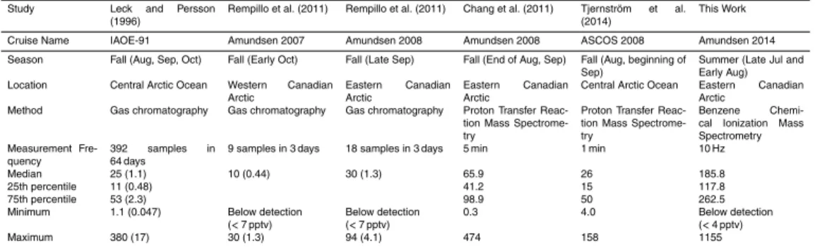
a few snapshots of DMSg in the Arctic exist from a handful of ship-board studies con-ducted over the last twenty years, none of which captured the most biologically pro-ductive time of June and July (Leck and Persson, 1996; Rempillo et al., 2011; Chang et al., 2011; Tjernström et al., 2014). The data span great distances in time and space and provide only a fragmented picture of tropospheric DMS levels in the Arctic.
Under-10
standing present-day sources of DMS is also relevant for predicting how these sources may change in a future climate. The goals of this study are (1) to present ship-board DMSg measurements taken in the Canadian Arctic during July and August 2014, and (2) to identify sources for the measured DMSg.
The intermediate lifetime of DMSg against OH oxidation of 1–2 days means that
15
whether it travels far before being oxidized or remains in the same area depends strongly on atmospheric transport patterns. Atmospheric transport mixes DMSgwithin the region, effectively smoothing out atmospheric concentration inhomogeneities due to inhomogeneity in the surface water DMS (referred to henceforth as DMSsw).
Trans-port can also bring DMSg from regions further afield. For example, a study by Nilsson
20
and Leck (2002) highlighted the importance of transport in bringing DMSgfrom regions of open water to regions covered by sea ice within the Arctic.
Despite the potential for an important role for atmospheric transport, few source apportionment studies for sulfur in the Arctic have been carried out. Previous work has focused almost exclusively on the aerosol phase. A common assumption that all
25
methane sulfonic acid (MSA) in the aerosol phase arises from oxidation of marine biogenic DMSg (Sharma et al., 2012). However, Hopke et al. (1995) suggested that
wet-ACPD
15, 35547–35589, 2015DMS in the Canadian Arctic
E. L. Mungall et al.
Title Page
Abstract Introduction
Conclusions References
Tables Figures
◭ ◮
◭ ◮
Back Close
Full Screen / Esc
Printer-friendly Version Interactive Discussion
Discussion
P
a
per
|
Discussion
P
a
per
|
Discussion
P
a
per
|
Discussion
P
a
per
|
lands and lakes are less important than oceanic emissions (Bates et al., 1992; Watts, 2000). However, these studies are based on very few or even no measurements in the Canadian North, and the fluxes for the Canadian tundra and boreal forest, which cover a very large surface area, are highly unconstrained. Much of the Arctic Ocean is in close proximity to land and is more subject to terrestrial influence than the open ocean
5
in other regions of the world (Macdonald et al., 2015).
Sources of DMSg other than seawater are not typically included in chemical trans-port and climate models, despite evidence in the literature for several other sources of DMSg. For example, significant levels of DMS have been measured in Canadian lakes (Sharma et al., 1999a; Richards et al., 1994). DMS emissions have also been
10
observed from various continental sources such as lichens (Gries et al., 1994), crops such as corn (Bates et al., 1992), wetlands (Nriagu et al., 1987), and biomass burning (Meinardi et al., 2003; Akagi et al., 2011). Terrestrial plants can be an important source of DMS as demonstrated by DMS levels in the hundreds of pptv range measured from creosote bush in Arizona and from trees and soils in the Amazonian rain forest
(Jar-15
dine et al., 2010, 2014). One previous study based on sulfur isotopes from Greenland included pooled biogenic continental and volcanic sources (as their isotopic signatures are not easily distinguishable) and estimated this continental component to be 44 % (Patris et al., 2002). In addition to the possibility of a continental source, melt ponds have been suggested as a potentially important source of DMS to the atmosphere
20
(Levasseur, 2013). These fresh or brackish ponds form from snow melt on top of the sea ice in spring and summer, and have been observed to have an extremely large areal extent, covering 30 % of the sea ice on average in midsummer with up to 90 % coverage in some regions (Rosel and Kaleschke, 2012). Here we present sensitivity studies to examine the potential importance of these alternative sources of DMSg.
25
Section 2 outlines our measurement methodology. Section 3 presents the measured DMSg time series along 3 weeks of the cruise. Section 3 also includes concurrent
measurements of DMSswand the calculated DMS air-sea flux estimates for the region.
ACPD
15, 35547–35589, 2015DMS in the Canadian Arctic
E. L. Mungall et al.
Title Page
Abstract Introduction
Conclusions References
Tables Figures
◭ ◮
◭ ◮
Back Close
Full Screen / Esc
Printer-friendly Version Interactive Discussion
Discussion
P
a
per
|
Discussion
P
a
per
|
Discussion
P
a
per
|
Discussion
P
a
per
|
dispersion model to interpret these measurements. Section 4 includes an examination of source regions for the measured DMSg and sensitivity studies related to possible
terrestrial sources.
2 Methods
2.1 Measurements
5
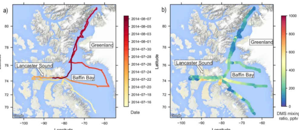
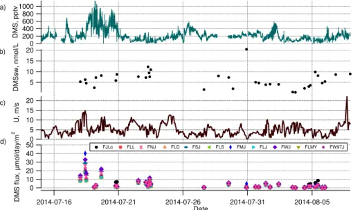
Measurements of DMS were made during the first leg of the CCGS Amundsen summer campaign under the aegis of NETCARE (Network on Climate and Aerosols: Address-ing Uncertainties in Remote Canadian Environments). The research cruise started in Quebec City on 8 July 2014 and ended in Kugluktuk on 14 August 2014. Measure-ments were made in Baffin Bay, Lancaster Sound and Nares Strait. The ship track is
10
shown in Fig. 1a.
2.1.1 DMS mixing ratios
DMSg measurements were made using a high resolution time of flight chemical
ion-ization mass spectrometer (HR-ToF-CIMS, Aerodyne). The instrument was housed in a container on the foredeck. The inlet was placed on a tower 9.44 m above the deck
15
at the bow, which was itself nominally 6.6 m a.s.l. (in total ca. 16 m a.s.l.). A diaphragm pump pulled air at 30 standard L min−1 through a 25 m long, 9.53 mm inner diameter PFA line heated to 50◦C (Clayborn Labs). Flow rate through the line was controlled by a critical orifice. The flow was subsampled and pulled to the instrument inlet through another critical orifice restricting the flow to 2 standard L min−1. The flow through the
20
sealed 210Po source of the HR-ToF-CIMS, also controlled at 2 standard L min−1 by a critical orifice, was supplied by a zero air generator (Parker Balston, Model HPZA-18000, followed by a Carbon Scrubber P/N B06-0263) via a mass flow controller sup-plying 2.4 standard L min−1. The zero air generator also supplied 9.8 sccm (controlled by a mass flow controller) through a bubbler filled with benzene, which was added to
ACPD
15, 35547–35589, 2015DMS in the Canadian Arctic
E. L. Mungall et al.
Title Page
Abstract Introduction
Conclusions References
Tables Figures
◭ ◮
◭ ◮
Back Close
Full Screen / Esc
Printer-friendly Version Interactive Discussion
Discussion
P
a
per
|
Discussion
P
a
per
|
Discussion
P
a
per
|
Discussion
P
a
per
|
the flow through the radioactive source to provide the reagent ion. The excess went to exhaust. Figure S1 in the Supplement shows a flow schematic.
The use of benzene cations as a reagent ion for chemical ionization mass spec-trometry was first proposed by Allgood et al. (1990). This reagent ion was successfully applied to the shipboard detection of DMS by the group of Tim Bertram at UCSD (Kim
5
et al., 2015). The ionization mechanism that prevails is the transfer of charge from a benzene cation to an analyte ion which has an ionization energy lower than that of benzene (Allgood et al., 1990). Due to space constraints on board the ship, a zero air generator was used instead of cylinder nitrogen to produce our reagent ion flows. The use of zero air introduced other potential reagent ions to the mass spectrum (O+2, NO+,
10
C6H+7, and H2O·H3O+, shown in Fig. S2 in the Supplement). To investigate the effect
of this more complicated reagent ion source, calibration experiments were carried out in the laboratory prior to the campaign for both air and N2at different sample flow
rela-tive humidities and under different CIMS voltage configurations. The calibration curves for DMS (detected as CH3SCH+3) showed a linear response under all conditions. We
15
found that the sensitivity of the instrument to DMS did not depend on relative humidity, and for operating conditions in the field averaged about 80 cps pptv−1
with detection limits below 4 pptv due to the background being in the 2–3 pptv range.
Background spectra were collected in the field by overflowing the inlet with zero air from the zero air generator as shown in Fig. S1. The high mass resolution of the
in-20
strument eliminated concern about isobaric interferences as indicated in Fig. S3 in the Supplement. Mass spectra were collected at 10 Hz. One point calibrations were performed nearly every day by overflowing the inlet with zero air and adding a known amount of DMS from a standards cylinder using a mass flow controller (499±5 %
ppb, Apel-Reimer). Peak fitting was performed using the Tofware software package
25
ACPD
15, 35547–35589, 2015DMS in the Canadian Arctic
E. L. Mungall et al.
Title Page
Abstract Introduction
Conclusions References
Tables Figures
◭ ◮
◭ ◮
Back Close
Full Screen / Esc
Printer-friendly Version Interactive Discussion
Discussion
P
a
per
|
Discussion
P
a
per
|
Discussion
P
a
per
|
Discussion
P
a
per
|
filtered such that values were removed when the ship was moving (speed over ground greater than 2 m s−1) and the wind direction was not within±90◦of the bow. This was
intended to remove artifacts that might have occurred due to enhanced DMS flux in the ship’s wake. This removed less than 12 % of data points.
2.1.2 Surface seawater DMS concentrations
5
Seawater concentrations of DMS were determined following procedures described by Scarratt et al. (2000) and modified in Lizotte et al. (2012) using purging, cryotrapping and sulfur-specific gas chromatography. Briefly, seawater was gently collected directly from 12 L Niskin bottles in gas-tight 24 mL serum vials, allowing the water to overflow. Subsamples of DMS were withdrawn from the 24 mL serum vials within minutes of
10
collection and sparged using an in line purge and trap system with a Varian 3800 gas chromatograph (GC) equipped with a pulsed flame photometric detector (PFPD). The GC was calibrated with injections of a 100 nM solution of hydrolyzed DMSP (Research Plus Inc.). The full dataset will be presented separately (M. Lizotte et al., personal communication, 2015).
15
2.1.3 Meteorological data
Basic meteorological measurements were made from a purpose built tower on the ship’s foredeck. Air temperature (8.2 m above deck), wind speed and direction (9.4 m above deck) and barometric pressure (1.5 m above deck) were measured using, re-spectively, a shielded temperature and relative humidity probe (Vaisala™HMP45C212),
20
wind monitor (RM Young 05103) and pressure transducer (RM Young™61205V). Sen-sors were scanned every 2 s and saved as 2 min averages to a micrologger (Campbell Scientific™model CR3000). Platform relative wind was post-processed to true wind fol-lowing Smith et al. (1999). Navigation data (ship position, speed over ground, course over ground and heading) necessary for the conversion were available from the ship’s
25
sen-ACPD
15, 35547–35589, 2015DMS in the Canadian Arctic
E. L. Mungall et al.
Title Page
Abstract Introduction
Conclusions References
Tables Figures
◭ ◮
◭ ◮
Back Close
Full Screen / Esc
Printer-friendly Version Interactive Discussion
Discussion
P
a
per
|
Discussion
P
a
per
|
Discussion
P
a
per
|
Discussion
P
a
per
|
sors were serviced or when the platform relative wind was beyond±90◦from the ship’s
bow were screened from the meteorological data set. Screened periods accounted for less than 20 % of total data but up to 45 % in some regions.
2.1.4 Sea surface temperature and salinity
Sea surface temperature (SST) was measured with the ship’s Inboard Shiptrack Water
5
System, Seabird/Seapoint measurement system. There were no continuous salinity measurements. An average salinity value of 29.7 PSU was used for all calculations since the calculated transfer velocities had very low sensitivity to changes in salinity for our study region.
2.2 Modeling
10
2.2.1 FLEXPART-WRF
A Lagrangian particle dispersion model based on FLEXPART (Stohl et al., 2005), FLEXPART-WRF (Brioude et al., 2013, website: flexpart.eu/wiki/FpLimitedareaWrf), was used to study the origin of air sampled by the ship. The model is driven by mete-orology from the Weather Research and Forecasting (WRF) Model (Skamarock et al.,
15
2005) and was run in backward mode to study the emissions source regions and trans-port pathways influencing ship-based DMS measurements. Specific details are in an-other publication arising from the NETCARE Amundsen campaign (Wentworth et al., 2015).
2.2.2 GEOS-Chem
20
The GEOS-Chem chemical transport model (http://www.geos-chem.org) was used to interpret the atmospheric measurements. We used GEOS-Chem version 9-02 at 2◦×2.5◦ resolution with 47 vertical layers between the surface and 0.01 hPa. The
Administra-ACPD
15, 35547–35589, 2015DMS in the Canadian Arctic
E. L. Mungall et al.
Title Page
Abstract Introduction
Conclusions References
Tables Figures
◭ ◮
◭ ◮
Back Close
Full Screen / Esc
Printer-friendly Version Interactive Discussion
Discussion
P
a
per
|
Discussion
P
a
per
|
Discussion
P
a
per
|
Discussion
P
a
per
|
tion (NASA) Global Modeling and Assimilation Office (GMAO) Goddard Earth Observ-ing System version 5.7.2 (GEOS-FP) assimilated meteorology product, which includes both hourly surface fields and 3 hourly 3-D fields. Our simulations used 2014 meteorol-ogy and allowed a 2 month spin-up prior to the simulation of July and August 2014.
The GEOS-Chem model includes a detailed oxidant-aerosol tropospheric chemistry
5
mechanism as originally described by Bey et al. (2001). Simulated aerosol species include sulphate-nitrate-ammonium (Park et al., 2004, 2006), carbonaceous aerosols (Park et al., 2003; Liao et al., 2007), dust (Fairlie et al., 2007, 2010) and sea salt (Alexander et al., 2005). The sulphate-nitrate-ammonium chemistry uses the ISOR-ROPIA II thermodynamic model (Fountoukis and Nenes, 2007), which partitions
am-10
monia and nitric acid between the gas and aerosol phases. The model includes natural and anthropogenic sources of SO2 and NH3 (Fisher et al., 2011b). DMS emissions
are based on the Liss and Merlivat (1986) sea–air flux formulation and oceanic DMS concentrations from Lana et al. (2011). In our simulations, DMS emissions occurred only in the fraction of the grid box that is covered by sea water and also free of sea
15
ice. Biomass burning emissions are from the Quick Fire Emissions Dataset (QFED2) (Darmenov and da Silva, 2013), which provides daily open fire emissions at 0.1◦
×0.1◦.
Oxidation of SO2occurs in clouds by reaction with H2O2and O3and in the gas phase
with OH (Alexander et al., 2009) and DMS oxidation occurs by reaction with OH and NO3.
20
The GEOS-Chem model has been extensively applied to study the Arctic including for aerosol acidity (Wentworth et al., 2015; Fisher et al., 2011a), carbonaceous aerosol (Wang et al., 2011), aerosol number (Croft et al., 2015), aerosol absorption (Breider et al., 2014), and mercury (Fisher et al., 2012).
2.2.3 Seawater DMS values in GEOS-Chem
25
The DMSsw values used in the standard GEOS-Chem are monthly means from the
ACPD
15, 35547–35589, 2015DMS in the Canadian Arctic
E. L. Mungall et al.
Title Page
Abstract Introduction
Conclusions References
Tables Figures
◭ ◮
◭ ◮
Back Close
Full Screen / Esc
Printer-friendly Version Interactive Discussion
Discussion
P
a
per
|
Discussion
P
a
per
|
Discussion
P
a
per
|
Discussion
P
a
per
|
predicts values of DMSsw below 5 nM in this region, while the values measured on board the ship during the campaign were often between 5–10 nM and occasionally higher. Therefore, we used the measured values as input in GEOS-Chem in lieu of the Lana et al. (2011) values for the study region. The measured values were interpolated using the DIVA web application (http://gher-diva.phys.ulg.ac.be/web-vis/diva.html) and
5
a static field was used for July and August.
To our knowledge, there exist no measurements of DMSsw in the Hudson Bay Sys-tem (comprising Hudson Bay, Foxe Basin and the Hudson Strait; referred to as HBS hereafter). In order the assess the potential importance of this source region to DMSg further north, we used primary productivity as a proxy for DMSsw for lack of better
10
options. To the best of our knowledge, no accepted proxy for DMSsw exists, and the development of such a proxy, while extremely valuable, is beyond the scope of this work. The work of Ferland et al. (2011) found that the waters of Hudson Strait are as productive as those of the North Water (Northern Baffin Bay), while Hudson Bay and Foxe Basin are about a quarter as productive. For our simulation we set the DMSsw in
15
Hudson Strait to be equal to that measured in the North Water, and the DMSswin
Hud-son Bay and Foxe Basin to a quarter of that value. The values chosen here for DMSsw represent what we believe to be a plausible scenario. In the absence of measurements, it is not possible to further constrain what the DMSsw values might be in the Hudson
Bay System.
20
2.3 Flux estimate calculations
Concurrent measurements of DMS in the atmosphere and seawater along the ship track allow us to estimate the air-sea flux of DMS. The flux is defined as the rate of transfer of a gas across a surface, in this case the surface of the ocean. For liquid-gas surfaces, the flux is described by Eq. (1),
25
F =−KW Cg/KH−Cl
ACPD
15, 35547–35589, 2015DMS in the Canadian Arctic
E. L. Mungall et al.
Title Page
Abstract Introduction
Conclusions References
Tables Figures
◭ ◮
◭ ◮
Back Close
Full Screen / Esc
Printer-friendly Version Interactive Discussion
Discussion
P
a
per
|
Discussion
P
a
per
|
Discussion
P
a
per
|
Discussion
P
a
per
|
whereCgand Cl are the concentrations of the chemical species of interest in the gas
phase and liquid phase respectively,KW is the transfer velocity, and KH is the
dimen-sionless gas over liquid form of the Henry’s law constant (Johnson, 2010). The transfer velocityKW is described by Eq. (2),
KW=
1
ka
+KH
kw
−1
(2)
5
whereKW is composed of the single phase transfer velocities for both the water-side
(kw) and the air-side (ka), representing the rates of transfer in each phase.
The transfer velocity for each phase encapsulates the physical processes controlling the flux in that phase. For soluble gases, the air-side processes play a more important role, and become increasingly relevant with increasing solubility, while insoluble gases
10
exhibit exclusively water-side control (Wanninkhof et al., 2009). Air-sea fluxes are con-trolled by many different factors, which has led to the development of a proliferation of transfer velocity parameterizations, each addressing different issues. Some are physi-cally based, i.e. attempt to mathematiphysi-cally describe the processes at play, while others are developed by fitting experimental or field data. It is not clear whether
parameteriza-15
tions developed based on measurements of the flux of a given gas can be applied to other gases. For example, bubbles contribute less to the DMS flux than they do to the CO2flux, due to the limited solubility of carbon dioxide in water, and so
parameteriza-tions developed for CO2 might be expected to overestimate the DMS flux (Blomquist
et al., 2006).
20
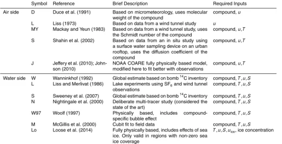
We used multiple transfer velocity parameterizations from the literature together with our measurements of atmospheric DMS mixing ratios, seawater DMS concentrations and wind speed to calculate fluxes. We compared these parameterizations to attempt to clarify the impact of the choice of parameterization on calculated fluxes. These pa-rameterizations are summarized in Table 1 and are referred to by acronyms of the form
25
parameteri-ACPD
15, 35547–35589, 2015DMS in the Canadian Arctic
E. L. Mungall et al.
Title Page
Abstract Introduction
Conclusions References
Tables Figures
◭ ◮
◭ ◮
Back Close
Full Screen / Esc
Printer-friendly Version Interactive Discussion
Discussion
P
a
per
|
Discussion
P
a
per
|
Discussion
P
a
per
|
Discussion
P
a
per
|
zation using the air-side parameterization of Jeffery et al. (2010) and the water-side parameterization of Liss and Merlivat (1986) is referred to as FJLM. The acronyms referring to the various parameterizations are listed in Table 1. Johnson implemented a wide variety (Table 1 provides details) of both air-side and water-side parameteri-zations (Johnson, 2010), all of which require only wind speed, air temperature, and
5
salinity as inputs. The relationship of the transfer velocity arising from each parameter-ization with wind speed for the conditions encountered during the cruise is shown in Fig. S4 in the Supplement. Loose et al. (2014) recently published a parameterization specific to the seasonal ice zone, incorporating ice-specific physical processes. This parameterization was used to calculate the water-side transfer velocity whenever the
10
ship was in the marginal ice zone, using estimated sea ice coverage and ice speeds. Sea ice cover near the ship’s location was estimated at a 0.5◦×0.5◦ resolution by
plotting the ship’s course at hourly resolution on daily ice charts obtained from the Canadian Ice Service (http://www.ec.gc.ca/glaces-ice/). These estimates were cross-referenced with daily photos taken aboard the ship to ensure accuracy. Estimates were
15
made on a scale from 1–10, with no fractional values. Ice speed was estimated using the relationship to wind speed found by (Cole et al., 2014),uice=0.019uair.
Fluxes were calculated according to Eq. (1) as the transfer velocity multiplied by the difference in concentration between the atmosphere and the ocean. Atmospheric con-centrations were calculated from measured mixing ratios using measured atmospheric
20
temperature and pressure and divided by the Henry’s law constant for DMS at the in situ temperature. Fluxes estimated by all transfer velocity parameterizations that did not explicitly include the effect of sea ice were multiplied by the fraction of open water in order to account for the capping effect of sea ice (Loose et al., 2014).
3 DMS mixing ratio observations and estimated fluxes
25
ACPD
15, 35547–35589, 2015DMS in the Canadian Arctic
E. L. Mungall et al.
Title Page
Abstract Introduction
Conclusions References
Tables Figures
◭ ◮
◭ ◮
Back Close
Full Screen / Esc
Printer-friendly Version Interactive Discussion
Discussion
P
a
per
|
Discussion
P
a
per
|
Discussion
P
a
per
|
Discussion
P
a
per
|
(July). These summertime measurements exceed previous measurements made in late summer and early fall by a factor of 3–10 (Table 2). This is consistent with the expectation of higher biological productivity in the summer than in other seasons (Lev-asseur, 2013). The time series shows high temporal variability. In particular, three episodes of elevated DMSg mixing ratios with values of 400 pptv or above occurred
5
along the ship track on 18–20 July, 26 July and 1–2 August. Two episodes of much lower DMSg mixing ratios with values below 100 pptv occurred on 22–23 July and 5 August. Comparing these measurements to those made in other regions of the world ocean indicates that our values are on the same order (hundreds of pptv) as measure-ments made at high latitudes under bloom conditions in the Southern Ocean (Bell et al.,
10
2015), the North Atlantic (Bell et al., 2013), and the North West Pacific (Tanimoto et al., 2013), but are higher than measurements made in the Tropical Pacific which were on the order of tens of pptv (Simpson et al., 2014).
Figure 2 presents the time series of DMS along the ship track together with the other variables needed to estimate fluxes (wind speed and seawater DMS concentrations)
15
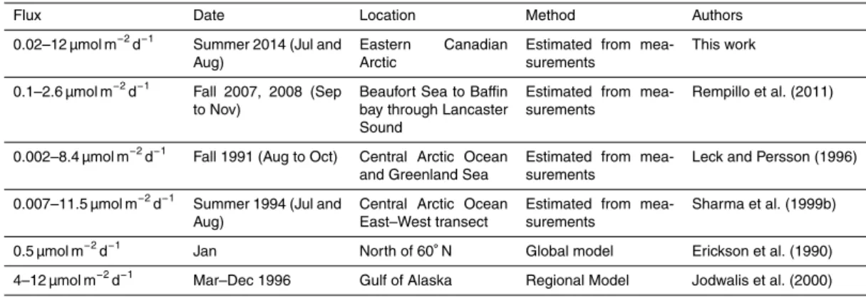
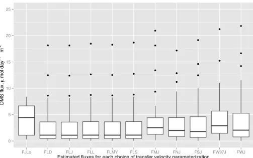
and shows the flux estimates as a time series for each transfer velocity parameter-ization used. Figure 3 shows the regional median DMS air-sea fluxes based on the ship track measurements for the Eastern Canadian Arctic summer. Previous DMS flux estimates for the Arctic are summarized in Table 3. The only other summertime esti-mate falls within the same range as in this work of ca. 0–10 µmol day−1m−2 (Sharma
20
et al., 1999b). Our values may represent an underestimate of the true regional flux, as wind speeds were low at the times when the highest DMSsw values were observed
on 23 and 31 July. It is probable that these high-DMSsw regions experienced higher wind speeds at other times, leading to a larger flux. A better constrained summer flux estimate for this region will require sampling of DMSsw at higher spatial and temporal
25
ACPD
15, 35547–35589, 2015DMS in the Canadian Arctic
E. L. Mungall et al.
Title Page
Abstract Introduction
Conclusions References
Tables Figures
◭ ◮
◭ ◮
Back Close
Full Screen / Esc
Printer-friendly Version Interactive Discussion
Discussion
P
a
per
|
Discussion
P
a
per
|
Discussion
P
a
per
|
Discussion
P
a
per
|
Figures 2 and 3 show that the choice of transfer velocity parameterization had little impact on the calculated fluxes the majority of the time, with the exception being times at which wind speeds were high (greater than 10 m s−1) during the period of 18–19 July. In particular, the choice of air-side parameterization (the difference between FLL, FLD, FLMY, FLS and FLJ in Fig. 3) had very little impact on the estimated fluxes, as shown
5
by the similarity of the medians and distributions of the fluxes estimated using these different parameterizations. Without direct flux measurements, we cannot determine which water-side transfer velocity parameterization is the most accurate. However, re-cent studies have shown that the wind speed dependence of the DMS transfer velocity is close to linear (Huebert et al., 2010; Bell et al., 2013, 2015). As a result we chose
10
to use a linear dependence of transfer velocity on wind speed in our GEOS-Chem simulations following the Liss and Merlivat (1986) parameterization.
Ultimately, more data is needed in order to evaluate which transfer velocity param-eterization is most suited to modeling DMS fluxes, and whether this varies geograph-ically. For example, the FJLo parameterization, which explicitly includes the effects of
15
sea ice in the marginal ice zone, predicts fluxes a factor of 2 larger than the other parameterizations do. This serves as a hint that accounting for the effect of sea ice on air-sea exchange in models (beyond a simple capping effect) may be important to modeling emissions of climatologically active gases such as DMS. Even without the additional consideration of regional differences such as sea ice cover, considerable
20
uncertainty concerning transfer velocity parameterizations remains. It is probable that all of the factors controlling air-sea flux are not yet understood (Johnson et al., 2011), and would in any case be very difficult to model. Accurate parameterization of sea–air fluxes is an active area of research, and advances in the field are essential to chemical transport models.
ACPD
15, 35547–35589, 2015DMS in the Canadian Arctic
E. L. Mungall et al.
Title Page
Abstract Introduction
Conclusions References
Tables Figures
◭ ◮
◭ ◮
Back Close
Full Screen / Esc
Printer-friendly Version Interactive Discussion
Discussion
P
a
per
|
Discussion
P
a
per
|
Discussion
P
a
per
|
Discussion
P
a
per
|
4 Source apportionment with GEOS-Chem and FLEXPART
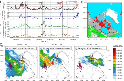
In order to explore the provenance of the air masses being sampled on the ship, we used FLEXPART-WRF backward runs as well as GEOS-Chem simulations. Figure 4 summarizes our understanding of the origins of air masses arriving at the ship track. Figure 4a shows the time series of DMSg from the GEOS-Chem simulation
superim-5
posed on the measured DMSgtime series, as well as the GEOS-Chem sea salt (a ma-rine tracer) and methyl ethyl ketone and carbon monoxide (MEK and CO, biomass burning tracers) mixing ratios. Figure 4b shows the main land cover types in the re-gion. Panel c in Fig. 4 shows examples of potential emissions sensitivity plots gener-ated using FLEXPART-WRF that indicate regions the air has passed over before being
10
sampled. Periods highlighted with a gray bar and numbered 1 through 3 were chosen as representative of three types of influence: (1) marine influence from south of the Arctic circle, (2) terrestrial influence from Northern Canada, and (3) regional marine influence from Baffin Bay. Sea salt tracer maxima indicate marine-influenced air and reflect high winds, while MEK and CO maxima indicate an influence from biomass
burn-15
ing. Biomass burning tracers provide a convenient indication of continental influence on the airmass. Figure 4 shows agreement between the sources of the air indicated by FLEXPART-WRF and by the GEOS-Chem tracers. For example, during Period 2 the MEK tracer is high and FLEXPART-WRF shows continental influence, while during Period 3 the sea salt tracer is high and FLEXPART-WRF shows marine influence.
20
4.1 Model-measurement comparison
Our GEOS-Chem simulations reproduce the major features of the measured DMSg time series, with appropriate magnitudes much of the time and an overall bias of
−67 pptv. The poorest model-measurement agreements occur on 1–2 and 6–7 August,
as shown in Figs. 5b and 4a, where GEOS-Chem overestimates DMS mixing ratios by
25
ACPD
15, 35547–35589, 2015DMS in the Canadian Arctic
E. L. Mungall et al.
Title Page
Abstract Introduction
Conclusions References
Tables Figures
◭ ◮
◭ ◮
Back Close
Full Screen / Esc
Printer-friendly Version Interactive Discussion
Discussion
P
a
per
|
Discussion
P
a
per
|
Discussion
P
a
per
|
Discussion
P
a
per
|
due to the DMSsw values for that time period being too large (given our use of a static field based on only a few measurements), to excessive GEOS wind speeds driving too large of a flux during this episode, or to errors in the parameterization used for the transfer velocity at high wind speeds. Wind speeds in our GEOS-Chem simulations are generally within a factor of 2 of the observed wind speeds along the ship track time
5
series. Overall, GEOS-Chem tended to overestimate DMSgin Baffin Bay (largely open water at the time of the campaign) and underestimate it in Lancaster Sound (where we encountered between 10–100 % ice cover). It is worth noting that the effect of sea ice on sea–air flux as hypothesized by Loose et al. (2014) is to increase the flux at low wind speeds and decrease it at high wind speeds. Implementation of this transfer velocity
10
parameterization might be expected to improve model-measurement agreement.
4.2 Local sources: Baffin Bay and Lancaster Sound
Figure 5a shows the relative contributions of various marine source regions to the GEOS-Chem simulation of the DMSg along the ship track. Nearly 90 % of the simu-lated DMS was contributed by the areas the ship was traveling through, Baffin Bay and
15
Lancaster Sound (shown in blue and purple respectively). These local emissions also contributed the majority of the highest mixing ratios observed during the campaign on 18 and 20 July. Overall, the waters of Baffin Bay and Lancaster Sound acted as a strong local source of DMSg throughout the campaign.
4.3 Transport: role of Hudson Bay System
20
Figure 5 shows that the influence of the HBS is significant on 18–19 July, contributing up to 60 % of simulated DMSg over that time period. This peak in DMS coincided with
a storm originating in lower latitudes blowing through Lancaster Sound, where the ship was located at the time. This transport pattern is visible in the FLEXPART-WRF retro-plume for Period 1 in Fig. 4c. These results suggest that DMS emissions from the HBS
25
atmo-ACPD
15, 35547–35589, 2015DMS in the Canadian Arctic
E. L. Mungall et al.
Title Page
Abstract Introduction
Conclusions References
Tables Figures
◭ ◮
◭ ◮
Back Close
Full Screen / Esc
Printer-friendly Version Interactive Discussion
Discussion
P
a
per
|
Discussion
P
a
per
|
Discussion
P
a
per
|
Discussion
P
a
per
|
sphere during episodic transport events associated with mid latitude storms traveling northward. This result depends on the assumption that the DMSsw values in the HBS are similar to levels observed at higher latitudes. However, the potential for influence from the HBS is supported by previous reports of high levels of DMS in air masses transported northward from the Hudson Bay region (Sjostedt et al., 2012).
Measure-5
ments of both DMSswand DMSg in the HBS are needed to confirm this hypothesis.
4.4 Investigation of possible missing sources
The GEOS-Chem simulated DMSgtime series fails to reproduce the peak in measured DMSg on 26 July (shown in Fig. 4a). This mismatch coincides with a minimum in the simulated marine tracer (sea salt), suggesting that a non-marine source of DMSg is
10
not being represented in the model. We expect DMSgand the sea salt tracer to covary in the model as their emissions are similarly dependent on wind speed and fraction of open ocean and their lifetimes are similarly short. It is possible that this disagreement indicates that the model does not capture the true relationship of DMSgto wind speed. However, the FLEXPART-WRF retroplumes for 26 July (an example is shown as Period
15
2 of Fig. 4c) indicate that the airmass had not traveled over very much open water be-fore reaching the ship’s location. This is supported by high levels of continental tracers (e.g. MEK, shown in the third panel of Fig. 4a) during these same periods.
The suggestion that DMSg may have a continental source is not new (Hopke et al., 1995), but it has not received very much attention. The FLEXPART-WRF PES
retro-20
plumes indicate that the continental area influencing the air masses sampled by the ship was Northern Canada (primarily, regions to the south and est of Baffin Bay, in-cluding Nunavut and the Northwest Territories). The land cover in that region is shown in Fig. 4b and is a mixture of tundra, boreal forest, wetlands and lakes. As well, there was a wide spatial extent of melt ponds to the south and west of the ship track (shown
25
ACPD
15, 35547–35589, 2015DMS in the Canadian Arctic
E. L. Mungall et al.
Title Page
Abstract Introduction
Conclusions References
Tables Figures
◭ ◮
◭ ◮
Back Close
Full Screen / Esc
Printer-friendly Version Interactive Discussion
Discussion
P
a
per
|
Discussion
P
a
per
|
Discussion
P
a
per
|
Discussion
P
a
per
|
possible. We implemented these extra emissions in the GEOS-Chem model and per-formed sensitivity tests to explore their potential contributions to DMSg at the ship
positions. These results are presented in the following subsections.
4.4.1 Emissions from melt ponds
Melt ponds form on the surface of sea ice as the snow melts. They cover much of
5
the surface of the sea ice by mid summer and have been suggested as a potentially important source of DMS to the atmosphere (Levasseur, 2013). At the time of the campaign, the sea ice regions to the west and south of our ship track, particularly in Lancaster Sound, had considerable melt pond coverage as shown in Fig. S5. The melt pond DMS source was implemented in GEOS-Chem by assuming that 50 % of sea ice
10
was covered by melt ponds and treating melt ponds as seawater in the model, that is, using the same flux parameterization as for open ocean (Liss and Merlivat, 1986). The validity of assuming the same flux parameterization applies to a shallow melt pond as to the open ocean is untested, but as discussed previously, the uncertainties associated with parameterizing transfer velocities in general are quite large, so we consider this
15
approximation reasonable for our sensitivity test. The concentration of DMSsw in the
melt ponds was set to 3 nM. This value was chosen to provide a reasonable upper limit based on measurements by Levasseur (2013).
The blue curve in Fig. 5c shows the modeled DMS contributed by the melt pond source. The melt pond contribution to the simulated DMSg time series at the ship track
20
was greatest during 18–25 July when the ship was in Lancaster Sound. The melt ponds contributed a maximum of 100 % to the total simulated DMSg at the ship position on 23 July when modeled and measured DMSg were very low. The strong contribution of the melt ponds at this time was likely due to the ship’s position at the ice edge and advection of the arriving airmass over ice-covered regions. The simulated melt
25
ACPD
15, 35547–35589, 2015DMS in the Canadian Arctic
E. L. Mungall et al.
Title Page
Abstract Introduction
Conclusions References
Tables Figures
◭ ◮
◭ ◮
Back Close
Full Screen / Esc
Printer-friendly Version Interactive Discussion
Discussion
P
a
per
|
Discussion
P
a
per
|
Discussion
P
a
per
|
Discussion
P
a
per
|
background levels of DMSg. More measurements of DMS concentrations in melt ponds and, ideally, direct measurements of DMS fluxes from melt ponds will further constrain the impact this source might have on DMSg in the Arctic summer.
4.4.2 Emissions from coastal tundra
Previous studies suggest that DMS emissions from lichens (Gries et al., 1994) and from
5
coastal tundra, particularly in regions where snow geese breed (Hines and Morrison, 1992), may be quite large. For lichens to emit reduced sulfur to the atmosphere, they require a source of sulfur. In coastal regions this can be supplied by sea spray. We im-plemented a tundra DMS source in GEOS-Chem by using the Olson Land Cover data (http://edc2.usgs.gov/glcc/globdoc2_0.php) to calculate the fraction of each
GEOS-10
Chem grid box covered by the land type “barren tundra”. We then assumed that 40 % of that tundra (to account for inland regions emitting less due to less sulfate being de-posited by sea spray) emitted DMS at a rate of 480 nM m−2h−1 (Hines and Morrison, 1992). We consider this simulation to give us an upper limit to the potential influence of tundra DMS emissions.
15
The results are presented as the brown curve in Fig. 5c. The simulated DMSg at the ship track had the largest contribution from tundra sources during 16–17 July, with a maximum contribution to the simulated DMSgat the ship position of 6 %. The percent contribution was lower than that of the melt pond source because the tundra source acted to increase simulated DMSg during times when levels were already high, but as
20
can be seen in Fig. 5c the absolute contribution of the modeled tundra source was comparable to or larger than the melt pond source contribution. Like the melt pond source, the possible tundra source reduces the overall normalized mean bias (by 14 %) and may contribute to the regional background levels of DMSg. However, neither source can account for the large unexplained peaks in the measured time series.
ACPD
15, 35547–35589, 2015DMS in the Canadian Arctic
E. L. Mungall et al.
Title Page
Abstract Introduction
Conclusions References
Tables Figures
◭ ◮
◭ ◮
Back Close
Full Screen / Esc
Printer-friendly Version Interactive Discussion
Discussion
P
a
per
|
Discussion
P
a
per
|
Discussion
P
a
per
|
Discussion
P
a
per
|
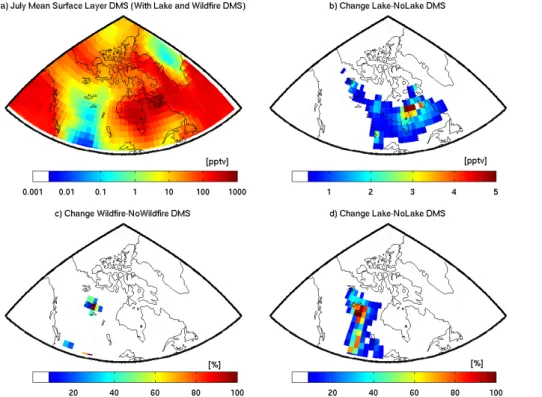
4.4.3 Emissions from lakes
To evaluate the potential contribution of DMS from lakes, the fresh water fraction in each GEOS-Chem grid box in a rectangular domain spanning 48 to 75◦N and−68 to −140◦W was calculated using the Olson Land Cover map, which has a resolution of
1 km. Based on the work of Sharma et al. (1999a), we assigned a mean value of 1 nM
5
DMS to the fresh water in that domain. We then applied the same Liss and Merlivat parameterization as was used to represent the air-water flux for the oceans to the frac-tion of the grid box with lake coverage. The same caveats apply to the use of transfer velocity parameterizations developed for the open ocean for fluxes from lakes as to the application to melt ponds as discussed above. Under these conditions, the lake source
10
was regionally important as shown in Fig. 6. It resulted in a modest increase in the absolute magnitude of DMSg in Northern Quebec and Labrador, and had negligible ef-fects elsewhere. The percent change in surface layer DMSgin the Northwest Territories was quite large due to there being no other sources of DMSgin that location in
GEOS-Chem, but the absolute values of DMSg are very small. The effect on the simulated
15
DMSg time series along our ship track in the Arctic is negligible. However, as there are so few measurements of DMS concentrations in lakes in Northern Canada, we cannot exclude the possibility that the actual lake concentrations of DMSsw are much higher
than 1 nM and that the unexplained peak in our time series is due to a lake source of DMSg. This possibility is supported by high chlorophyll-αlevels in the lakes of Northern
20
Canada (shown in Fig. S6 in the Supplement) and the fact that the measurements of DMSswin lakes that we used for this sensitivity test were made more than 15 years ago, and the high northern latitudes have warmed significantly since then (IPCC, 2013).
4.4.4 Emissions from forests and soils
Due to the paucity of measurements of DMS emissions from vegetation, boreal soils,
25
ACPD
15, 35547–35589, 2015DMS in the Canadian Arctic
E. L. Mungall et al.
Title Page
Abstract Introduction
Conclusions References
Tables Figures
◭ ◮
◭ ◮
Back Close
Full Screen / Esc
Printer-friendly Version Interactive Discussion
Discussion
P
a
per
|
Discussion
P
a
per
|
Discussion
P
a
per
|
Discussion
P
a
per
|
tracers in GEOS-Chem shown in Fig. 4a suggests that the missing DMS was being co-transported with these biomass burning tracers. The measurement-model diff er-ence and the MEK tracer have a similar peak on 26 July as shown in Fig. 4a. The FLEXPART-WRF retroplumes (e.g. Period 2 in Fig. 4) identify this time as being conti-nentally influenced.
5
DMS emissions have been reported from biomass burning (Akagi et al., 2011; Meinardi et al., 2003) and summer 2014 saw a particularly active wildfire season in Northern Canada (Blunden and Arndt, 2015). The simplest reason for the maxima in biomass burning tracers during the unexplained DMSgpeak on 26 July would be emis-sions of DMS from biomass burning that are not represented in the model. To gauge
10
the importance of this source to DMSg in the Arctic, we used the emission factor for DMS from boreal forest biomass burning reported by Akagi et al. (2011). We indexed the DMS emissions to CO emissions, such that 3.66×10⁻⁵molecules of DMS are
emit-ted for each molecule of CO emitemit-ted in GEOS-Chem. Figure 6 shows that the biomass burning sensitivity test showed that the biomass burning source of DMSg had local
15
influence only, like the modeled lake source. The reason for this is that the emission factor for DMS from boreal forest fires is not very large. As a result, this source acted to increase DMSg in the immediate vicinity of the wildfires in the Northwest Territories, but had a negligible influence on the time series and is therefore not shown in Fig. 5. The biomass burning source of DMSg was likely not sufficient to directly influence the
20
DMSg time series at the ship position, unless the emission factor used in the model is an order of magnitude too low. This seems unlikely as the emission factor we used was derived from direct measurements in a biomass burning plume originating from the boreal forest (Akagi et al., 2011), but remains a possibility as much higher DMS emissions have been measured from other types of biomass burning in other locations
25
(Meinardi et al., 2003).
Further evidence for DMSg being co-transported with biomass burning tracers is
ACPD
15, 35547–35589, 2015DMS in the Canadian Arctic
E. L. Mungall et al.
Title Page
Abstract Introduction
Conclusions References
Tables Figures
◭ ◮
◭ ◮
Back Close
Full Screen / Esc
Printer-friendly Version Interactive Discussion
Discussion
P
a
per
|
Discussion
P
a
per
|
Discussion
P
a
per
|
Discussion
P
a
per
|
to the simulated DMSg. The result of this addition is to decrease the measurement-model bias by 24 % overall, and to reduce the residual by 200 pptv during the 26 July period of interest. The time series of additional DMSg is shown as the green curve in Fig. 5c. Alternatively, the air mass observed at the ship could have passed over a strong near-land marine source, which is missing in our simulations. The region air
5
mass passed over, however, was nearly entirely ice-covered at the time, making this an unlikely explanation for the observed DMSg. These results cannot tell us anything about the nature of the continental source, but they highlight the possibility that a source linked in some way to terrestrial flora could have an important effect on DMSg in the Arctic summer.
10
Emissions of reduced sulfur species from both soils and lakes are temperature de-pendent (Bates et al., 1992), opening up the possibility that the wild fires were indirectly promoting DMS emissions. Proximity to wild fires would tend to increase the temper-ature of the soil as well as changing the quality of the air in a way that might stress biota. A mechanism whereby biomass burning increases the emission of reduced
sul-15
fur species such as DMS from soils, lakes and vegetation might yield increased emis-sions but this requires further study and we do not have any information that would allow implementation of this possible effect in our simulations.
5 Conclusions
Interpreting our recent shipboard DMSg measurements with the GEOS-Chem
chemi-20
cal transport model, we have shown that local oceanic sources can account for a large proportion (70 %) of the atmospheric surface-layer DMS measured along our ship track in the Canadian Arctic Archipelago and Baffin Bay during summer 2014, and that the ocean was acting as a strong local source of DMSg. With GEOS-Chem simulations, we have also shown that marine sources south of the Arctic Circle episodically contribute
25
ACPD
15, 35547–35589, 2015DMS in the Canadian Arctic
E. L. Mungall et al.
Title Page
Abstract Introduction
Conclusions References
Tables Figures
◭ ◮
◭ ◮
Back Close
Full Screen / Esc
Printer-friendly Version Interactive Discussion
Discussion
P
a
per
|
Discussion
P
a
per
|
Discussion
P
a
per
|
Discussion
P
a
per
|
formation from DMS has been argued convincingly in a global sense by Quinn and Bates (2011). We propose that it may also be important episodically in the Arctic, e.g. transport from the Hudson Bay System or the Northwest Territories. These origins for air at our ship track are also supported by FLEXPART-WRF retroplume analysis.
Overall, source apportionment using FLEXPART-WRF and GEOS-Chem indicate
5
that local sources dominate atmospheric DMS in the Canadian Arctic Archipelago and Baffin Bay. However, GEOS-Chem simulations show a low bias of 67 pptv over the ship track time series (from 10 to 100 % of the measured mixing ratios). We investigated sev-eral alternative sources that could act to correct this bias and presented evidence that some of these sources make a non-negligible contribution to surface layer DMS mixing
10
ratios. This included sources from tundra, forests, lakes and melt ponds. Our sensitiv-ity simulations indicated maximum contributions of 6 and 100 % from tundra and melt ponds, respectively, to our DMSgtime series at the ship position, suggesting that emis-sions of DMS from melt ponds and coastal tundra could have important local, regional effects on DMS levels. Given our confidence in marine-based DMS sources, we also
15
estimated as much as 94 % of the DMSg at the ship position could be from terrestrial sources (or another source missing from the model) during episodic transport events. These emissions may be related to changes in lake, forest and soil emissions due to the heat and stress associated with biomass burning. Flux measurements from melt ponds and the boreal forest and lakes, particularly when under stress from biomass
20
burning events, are needed to constrain this missing source.
Our findings have implications for our understanding of the sulfur cycle in the summer Arctic and how it has changed in the recent past and will continue to change in the future. For example, much of the discussion surrounding changes in Arctic DMS has focused on the loss of sea ice (Levasseur, 2013), but the loss of permafrost might also
25
ACPD
15, 35547–35589, 2015DMS in the Canadian Arctic
E. L. Mungall et al.
Title Page
Abstract Introduction
Conclusions References
Tables Figures
◭ ◮
◭ ◮
Back Close
Full Screen / Esc
Printer-friendly Version Interactive Discussion
Discussion
P
a
per
|
Discussion
P
a
per
|
Discussion
P
a
per
|
Discussion
P
a
per
|
The Supplement related to this article is available online at doi:10.5194/acpd-15-35547-2015-supplement.
Acknowledgements. The authors would like to acknowledge the financial support of NSERC for
the NETCARE project funded under the Climate Change and Atmospheric Research program. As well, we thank ArcticNet for hosting NETCARE scientists on the Amundsen, in particular
5
the help of Keith Levesque, and all of the crew and scientists aboard. Additionally, special thanks to Amir Aliabadi, Ralf Staebler, Lauren Candlish, Heather Stark, Tonya Burgers and Tim Papakyriakou for ozone sondes and meteorological data. Thanks to Michelle Kim and Tim Bertram of UCSD for invaluable discussions of ion chemistry. The authors thank K. Tavis and P. Kim for their assistance in implementation of the QFED2 database.
10
References
Akagi, S. K., Yokelson, R. J., Wiedinmyer, C., Alvarado, M. J., Reid, J. S., Karl, T., Crounse, J. D., and Wennberg, P. O.: Emission factors for open and domestic biomass burning for use in atmospheric models, Atmos. Chem. Phys., 11, 4039–4072, doi:10.5194/acp-11-4039-2011, 2011. 35551, 35568
15
Albrecht, B. A.: Aerosols, cloud microphysics, and fractional cloudiness, Science, 245, 1227– 1230, 1989. 35549
Alexander, B., Park, R. J., Jacob, D. J., Li, Q., Yantosca, R. M., Savarino, J., Lee, C., and Thiemens, M.: Sulfate formation in sea-salt aerosols: constraints from oxygen isotopes, J. Geophys. Res.-Atmos., 110, D10307, doi:10.1029/2004JD005659, 2005. 35556
20
Alexander, B., Park, R. J., Jacob, D. J., and Gong, S.: Transition metal-catalyzed oxidation of atmospheric sulfur: global implications for the sulfur budget, J. Geophys. Res.-Atmos., 114, D02309, doi:10.1029/2008JD010486, 2009. 35556
Allgood, C., Lin, Y., Ma, Y.-C., and Munson, B.: Benzene as a selective chemical ioniza-tion reagent gas, Org. Mass Spectrom., 25, 497–502, doi:10.1002/oms.1210251003, 1990.
25
35553
ACPD
15, 35547–35589, 2015DMS in the Canadian Arctic
E. L. Mungall et al.
Title Page
Abstract Introduction
Conclusions References
Tables Figures
◭ ◮
◭ ◮
Back Close
Full Screen / Esc
Printer-friendly Version Interactive Discussion
Discussion
P
a
per
|
Discussion
P
a
per
|
Discussion
P
a
per
|
Discussion
P
a
per
|
Bell, T. G., De Bruyn, W., Miller, S. D., Ward, B., Christensen, K. H., and Saltzman, E. S.: Air– sea dimethylsulfide (DMS) gas transfer in the North Atlantic: evidence for limited interfacial gas exchange at high wind speed, Atmos. Chem. Phys., 13, 11073–11087, doi:10.5194/acp-13-11073-2013, 2013. 35560, 35561
Bell, T. G., De Bruyn, W., Marandino, C. A., Miller, S. D., Law, C. S., Smith, M. J., and
Saltz-5
man, E. S.: Dimethylsulfide gas transfer coefficients from algal blooms in the Southern
Ocean, Atmos. Chem. Phys., 15, 1783–1794, doi:10.5194/acp-15-1783-2015, 2015. 35560, 35561
Bey, I., Jacob, D. J., Yantosca, R. M., Logan, J. A., Field, B. D., Fiore, A. M., Li, Q., Liu, H. Y., Mickley, L. J., and Schultz, M. G.: Global modeling of tropospheric chemistry with
as-10
similated meteorology: model description and evaluation, J. Geophys. Res., 106,23073, doi:10.1029/2001jd000807, 2001. 35556
Blomquist, B. W., Fairall, C. W., Huebert, B. J., Kieber, D. J., and Westby, G. R.: DMS sea-air transfer velocity: direct measurements by eddy covariance and parameteriza-tion based on the NOAA/COARE gas transfer model, Geophys. Res. Lett., 33, L07601,
15
doi:10.1029/2006GL025735, doi:10.1029/2006GL025735, 2006. 35558
Blunden, J. and Arndt, D. S.: State of the Climate in 2014, B. Am. Meteorol. Soc., 96, ES1– ES32, doi:10.1175/2015BAMSStateoftheClimate.1, 2015. 35568
Breider, T. J., Mickley, L. J., Jacob, D. J., Wang, Q., Fisher, J. A., Chang, R. Y.-W., and Alexander, B.: Annual distributions and sources of Arctic aerosol components,
20
aerosol optical depth, and aerosol absorption, J. Geophys. Res-Atmos., 119, 4107–4124, doi:10.1002/2013JD020996, 2014. 35556
Brioude, J., Arnold, D., Stohl, A., Cassiani, M., Morton, D., Seibert, P., Angevine, W., Evan, S., Dingwell, A., Fast, J. D., Easter, R. C., Pisso, I., Burkhart, J., and Wotawa, G.: The Lagrangian particle dispersion model FLEXPART-WRF version 3.1, Geosci. Model Dev., 6, 1889–1904,
25
doi:10.5194/gmd-6-1889-2013, 2013. 35555
Browse, J., Carslaw, K. S., Arnold, S. R., Pringle, K., and Boucher, O.: The scavenging pro-cesses controlling the seasonal cycle in Arctic sulphate and black carbon aerosol, Atmos. Chem. Phys., 12, 6775–6798, doi:10.5194/acp-12-6775-2012, 2012. 35549
Chang, R. Y.-W., Sjostedt, S. J., Pierce, J. R., Papakyriakou, T. N., Scarratt, M. G., Michaud, S.,
30
ACPD
15, 35547–35589, 2015DMS in the Canadian Arctic
E. L. Mungall et al.
Title Page
Abstract Introduction
Conclusions References
Tables Figures
◭ ◮
◭ ◮
Back Close
Full Screen / Esc
Printer-friendly Version Interactive Discussion
Discussion
P
a
per
|
Discussion
P
a
per
|
Discussion
P
a
per
|
Discussion
P
a
per
|
Charlson, R. J., Lovelock, J. E., Andreae, M. O., and Warren, S. G.: Oceanic phytoplankton, at-mospheric sulphur, cloud albedo and climate, Nature, 326, 655–661, doi:10.1038/326655a0, 1987. 35549
Chen, H., Ezell, M. J., Arquero, K. D., Varner, M. E., Dawson, M. L., Gerber, R. B., and Finlayson-Pitts, B. J.: New particle formation and growth from
methanesul-5
fonic acid, trimethylamine and water, Phys. Chem. Chem. Phys., 17, 13699—13709, doi:10.1039/C5CP00838G, 2015. 35549
Cole, S. T., Timmermans, M.-L., Toole, J. M., Krishfield, R. A., and Thwaites, F. T.: Ekman veering, internal waves, and turbulence observed under Arctic sea ice, J. Phys. Oceanogr., 44, 1306–1328, doi:10.1175/JPO-D-12-0191.1, 2014. 35559
10
Croft, B., Martin, R. V., Leaitch, W. R., Tunved, P., Breider, T. J., D’Andrea, S. D., and Pierce, J. R.: Processes controlling the seasonal cycle of Arctic aerosol number and size distributions, Atmos. Chem. Phys. Discuss., 15, 29079–29124, doi:10.5194/acpd-15-29079-2015, 2015. 35556
Darmenov, A. and da Silva, A.: The quick fire emissions dataset (QFED)–documentation of
15
versions 2.1, 2.2 and 2.4, NASA Technical Report Series on Global Modeling and Data Assimilation, NASA TM-2013-104606, 32, 183, 2013. 35556
Duce, R. A., Liss, P. S., Merrill, J. T., Atlas, E. L., Buat-Menard, P., Hicks, B. B., Miller, J. M., Pros-pero, J. M., Arimoto, R., Church, T. M., Ellis, W., Galloway, J. N., Hansen, L., Jickells, T. D., Knap, A. H., Reinhardt, K. H., Schneider, B., Soudine, A., Tokos, J. J., Tsunogai, S.,
Wol-20
last, R., and Zhou, M.: The atmospheric input of trace species to the world ocean, Global Biogeochem. Cy., 5, 193–259, doi:10.1029/91GB01778, 1991. 35581
Erickson, D. J., Ghan, S. J., and Penner, J. E.: Global ocean-to-atmosphere dimethyl sulfide flux, J. Geophys. Res.-Atmos., 95, 7543–7552, doi:10.1029/JD095iD06p07543, 1990. 35583 Fairlie, T. D., Jacob, D. J., and Park, R. J.: The impact of transpacific transport of mineral dust
25
in the United States, Atmos. Environ., 41, 1251–1266, 2007. 35556
Fairlie, T. D., Jacob, D. J., Dibb, J. E., Alexander, B., Avery, M. A., van Donkelaar, A., and Zhang, L.: Impact of mineral dust on nitrate, sulfate, and ozone in transpacific Asian pollution plumes, Atmos. Chem. Phys., 10, 3999–4012, doi:10.5194/acp-10-3999-2010, 2010. 35556 Ferland, J., Gosselin, M., and Starr, M.: Environmental control of summer primary
produc-30