Financial Sector Development, Economic Growth and Poverty
Reduction: New Evidence from Nigeria
Muhammad Yusuf DANDUME
Umaru Musa Yaradua University, Economic Department, Katsina State of Nigeria, dandumey@yahoo.com
Abstract
There is a common view that a well developed financial system will usher economic growth and further reduce the level of poverty. In late years the automaticity of this relationship in poor states such as Nigeria has been an area of considerable argument. This study attempts to examine this presuppose causal relationship between financial sector development, economic growth and poverty reduction in Nigeria. The study uses Autoregressive Distributed Lag model (ARDL) and Toda and Yamamoto No causality test, using a time series data covering the period of 1970-2011. The study includes poverty into the ongoing competing finance growth nexus hypothesis, in order to ascertain whether the poor segment of the Nigerian society have access to financial resources and also fully participate in the economic growth process in the country. Empirical results of the study reveal that financial sector development does not cause poverty reduction. This implies, increased in the supply of loan able funds due to financial sector development is not enough to ensure poverty reduction. Certain measures are important. Therefore, the results reveal, that economic growth causes financial sector growth. Implies that economic growth lead and financial sector follow. This implies that for financial sector development, economic growth is necessary, even though not sufficient for poverty reduction.
Keywords: Causality, Financial Depth, Growth, Co-Integration.
JEL Classification Codes: F21, F43.
Finansal Sektörde Gelişim, Ekonomik Büyüme, Yoksulluk Oranın Düşürülmesi: Nijerya
Örneği*
Öz
Büyüyen finansal sistem ve yoksulluğun azaltılması gelişmiş ekonomilerin en önemli özellikleri olarak karşımıza çıkmaktadır. Son yıllarda fakir ülkelerde, bu iki dinamik arasındaki ilişki tartışma konusu olmaya başlamıştır. Bu çalışma Nijerya’da finansal büyüme ve yoksulluk oranının düşürülmesi arasındaki ilişkiyi ARDL ve Toda, Yamamoto Modelleri’ni kullanarak ortaya koymayı amaçlamaktadır. 1970-2011 yılları arasındaki sürece ilişkin neden-sonuç ilişkisini ortaya
koyacak datalar mevcut değildir. Aynı zamanda çalışmada Nijerya toplumunun fakir kesiminin de finansal kaynaklara ulaşabildiği ve ülkenin ekonomik büyüme sürecine tamamıyla dahil olduğu analiz edilmektedir. Çalışmanın ampirik sonuçlarına göre finansal sektörün gelişmesi yoksulluk seviyesini düşürmemektedir. Finansal sektörün gelişimi yoksulluk seviyesinin düşürülmesine yönelik krediler alımını arttırmaktadır. Öte yandan, ekonomik büyüme beraberinde finansal büyümeyi de getirmektedir. Sonuç olarak, tek başına yoksulluk oranını azaltamasa da finansal
sektörün gelişimi için ekonomik büyüme şarttır.
Anahtar Kelimeler: Neden-Sonuç İlişkisi, Finansal Derinlik, Büyüme, Eşbütünleşme. JEL Sınıflandırma Kodları: F21, F43.
* The English title and abstract of this article has been translated into Turkish by the Editorial Board.
1. Introduction
Studies on the contribution of the financial sector to economic development focus much attention on the competing finance growth nexus. This is traced back to the seminal work of Schumpeter in (1911) who argued that a creation of credit through banking was a crucial factor of entrepreneur capabilities to drive growth. This idea sat well with many governments of Poor countries and sparked a mass of reforms in their financial sector Maduka & Onwuka, 2013). This also led to a spread of a substantial volume of studies (Otto Godly, 2012), but with much less emphasis on gaining and understanding of weather really, financial sector causes poverty reduction and whether finance growth nexus hypothesis can explain poverty reduction. Few questions appear to be resolved or largely undisputed (Odhiambo, 2010). In Nigeria, one of the salient properties of the recent economic growth performance is the reform exercise of the financial sectors. For example, the consolidation exercise in the banking sector plays a major role in the recent increase in the economic growth to the average of 7% since 2006. This apparent increase indicates that Nigerian economic growth is moving faster than the 6.5% Millennium development target goal for poverty reduction in sub-Saharan Africa (MDG, 2010). Surprisingly, despite this increased in economic growth, yet 51.6% of Nigerians were living below US$1 per day in 2004, and sharply increased to 61.2% in 2010. More so, inequality of income distribution rose from 0.429 in 2004 to 0.447 in 2010 (NBS, 2011). While the proportion of the extremely poor increased from 6.2 percent in 1980 to 29.3 percent in 1996 and then came down to 22.0 percent in 2004 before reaching 38.7% in 2010. In fact, the poor continue to be marginalized and deprived access to financial market (Yusuf, Malarvizhi & Khin, 2013). Nigeria is a veritable case for investigating to what extend does the financial sector contribute to economic growth and transforms economic growth into reduction of poverty. In fact, neglecting poverty in the studies of Nnanna (2004), Nzotta & Okerette (2009) constitute a serious measurement error of omission variable. This study contributes by adding poverty reduction in the ongoing debate on the finance-growth relationship.
1.1 The Financial Sector Development in Nigeria
The linkage between financial sector development, economic growth and poverty reduction can theoretically be established based on the two strands school of thought who emerged to explain the competing finance-growth and poverty reduction relationship. These are the financial regulation based versus financial deregulation based theoretical paradigm. According to the financial repression based theory, banking sector provide capital for economic growth and access to information to take up (Levine, 2002). On the other hand, the letter approach, pointed out that the market provides the efficient mediating role between financial sector development in one and economic growth in the other. Indeed, the unregulated financial sector was seen as the locomotive of economic development. This theory went further to explain that a sound and liquid financial market serves as engine economic growth and enable growth to transmit into poverty reduction (Levine, 2002). On the Nigeria scene the sector has passed through a various transformation from Independence to date. The era of 1950 to 1970 was the establishment era, when major commercial banks, including Central bank were established in the country. The structural Adjustment period, which was established in 1986, set the beginning of real financial sector transformational agenda. Before this time financial sector was highly repressed characterized by interest rate ceilings, selective credit expansion, control reserve requirement and various forms of direct monetary policy controls. Government owned, monopolized the banking industry with strict entrance regulation to the private sectors and regulated foreign exchange regime. However, with the implementation of Structural Adjustment Program there was a policy reversal toward the deregulation of the economy, by establishing the Nigerian deposit insurance corporation, putting in place corporate governance policies through tight supervisory institutions. Capital market was deregulated, and the indirect monetary policy instrument was introduced. The central bank took over the control of the distress banks in the country. Exchange rate reforms were put in place and this was achieved by establishing market based autonomous foreign exchange market. Reintroduction of exchange control in the 1994 but immediately after one year of its maturity, it was replaced back to the deregulated exchange regime. Similar goes to the interest rate regime which was capped in for a year and then reverses to the deregulated interest rate regime. Another major change was the deregulation of the banking sector; this was followed by the liberalization of the interest rate regime and the free entry of the banking business by the private individuals. This also led to the raised in the nominal interest rate in the country.
banking consolidation program banks are mandated by the Central Bank of Nigeria, to increase their capital based from the N2 billion amount to N250 billion. This was the aim of enhancing the availability of the loan able funds in the economy. Banking sector consolidation was to be supported with improvement in cooperating governance in terms of banking supervisory functions. The consolidation created a shift in the banking sector performance from efficient supervision to a risk based system strategy, based on the Based-11 Accord.
Referable to the overheating crisis on the financial sector emanating from the global melt down. Certain important reform measures were introduced, which includes, improving the quality of banks in role and contribution towards a sound financial sector and transforming the sector to play role toward the real sector performance. Despite all these measures put in placed the financial sector reforms and development do not translate into meaningful economic growth and poverty reduction (Yusuf et al., 2013). Instead the poverty rate in the nation continues to soar and the percent of the entire population in poverty continues to rise (NBS 2010). The relative poverty also continues to increase moving from 54.4 percent in 2004 to 69 percent in 2010 (NBS, 2010).
2. Literature Review
Theoretically, there are two strands school of thought which emerged to explain the competing finance-growth nexus. These are the banks based versus market based theoretical paradigm and the second was based on the law and finance based. According to the bank based theory, banking sector provide capital for economic growth and access to information to take up (Levine, 2002). On the other hand, the market friendly approach, pointed out that the market provides the efficient mediating role to the economic growth, in fact, the market was examined as the locomotive of economic development. This theory gave way further to demonstrate that a sound and liquid market provide higher economic growth and enable risk management and general diversification (Levine, 2002). So the finance friendly paradigm which was brought forth from the bank based approach stressed the importance of financial service provided by the financial organization. In the end, the last paradigm emphasized on the law based approach which stressed the important role of the sound system in creating growth (Upchurch, 2012).
On the empirical ground, studies in these perspectives, is divided into two dichotomies,
development. The argument that finance follows where enterprise leads are often followed in the work of Robin & Salina Martin (1992), these studies applied cross-sectional data, their studies provide pooled effects outcomes without providing details on country specific issues. Likewise, it neglected to get the dynamic effects between the two variables under investigation.
One of the outstanding studies on financial sector development and economic growth emerged from the works of Mehran (1998) who examine the progress recorded on the transformation of the financial sector of sub-saharan African countries. The findings suggest that financial sector development in Sub-Saharan African requires reforms in the area of financial supervision, financial development of the monetary operations and financial market. Marry, Chibuzo & Okelue (2012) investigate the effects as well as the relationship between financial sector development and economic development in Nigeria. The findings suggest a significant positive linkage between government consumption and trade openness. However, on the contrary the measures of financial development suggest a negative linkage with economic growth. In a related development Saibu, Nwosa & Agbeluyi (2011) investigate the effects of financial development and foreign direct investment on economic growth in Nigeria. The results indicate that there is a bidirectional causality relationship between some of the proxies of financial development and economic growth. Odeniran & Udeaja (2010) examine the relationship between financial sector development and economic growth in Nigeria, using Granger causality tests. The findings suggest bidirectional causality between financial sector development and economic growth in Nigeria.
Adam (2011) examines the impact of Ghana financial openness induced growth on poverty between 1970 and 2007. The finding suggests a positive relationship between growth and financial liberalization. On whether financial liberalization benefits the poor the findings suggest a positive relationship, but in a disproportionate manner. Therefore, on the basis of the findings they argued that credit channels are more efficient ways of addressing poverty if supported by a good policy intervention. Among the few studies supporting this argument is the study of Pradham (2010) who draw data from India and investigates the direction of the relationship between the financial sector, economic growth and poverty reduction for the period 1951-2008, through the technique of co -integration and causality test. The study finds a long run relationship running from finance to growth and poverty reduction. Odhihiambo (2009) using data from South Africa, established that economic growth granger causes financial development and, therefore, lead in the process of poverty reduction in South- Africa. Even though, the study suffers from measurement error by using granger frame work in the presence of small sample size, which consumes a lot degree of freedom, yet the study has been one of the few breakthrough studies in Africa. Ndebbio (2004) used ordinary least square regression techniques and the findings of the study provide an interesting revelation of a very weak relationship from finance to growth. This, according to him was attributed to poor and weak financial sector development in Nigeria. Alayande (2003) analyzed the patterns of inequality in Nigeria, using the regression-based approach to decompose inequality of income from sources using the Gini index. The findings of the studies suggest that geography contribute significantly in explaining poverty. The results of Alayande (2003) also show that the sector of residence alone accounted for the largest source of inequality in Nigeria. Therefore, went further to reveal that the level of education contributes significantly in explaining inequality of income. Alayande (2003) discovered that certain variables provide a little contribution such as the age and the sex of the respondents. Therefore, suggests that any policy on poverty reduction in Nigeria should give more emphasis to geographic distribution of the population. Obayelu & Awoyemi, (2012) applied regression decomposition techniques using National living standard survey data. The findings of the study attributes that household size contributes significantly to poverty.
3. Data and Methodology
3.1. Sources of Data
were source from the World development indicators. The data on Trade ration
were obtains from the World Bank Development Indicators.
Table 1: Variables and Their Source of Data
Symbol Variables Source
GDP Economic growth World Bank Development Indicators
FD Financial dept World Bank Development Indicators
RI Real interest rate World Development Indicators
TR Total value of export and
import
World Development Indicators
PO Poverty National bureau of statistics of Nigeria
Two approaches were used to ascertain the direction of influence between finance, growth and poverty nexus. The first approach involves the newly introduced ARDL approach to co- integration and causality. The second approach applied the Vector autoregressive (VAR) model with augmented lag order for the estimation of no causality Toda and Yamamoto test. The hypothesis of interest is that poverty reduction can be predicted by finance and growth interaction with the aid of certain control variables which includes interest rate, international trade and Real interest rate. However, based on the theoretical postulates a positive and significant coefficient estimate is expected. Therefore, following the work of Odhiambo (2009) and Pradhan (2010) the model is specified as follows:
0 1 3 4 5 (1)
GDPt FD RIt TRt POtKt
Where GDP is the proxy of economic growth, FD is the financial depth; RI is the real interest rate which is the deposits rate minus the inflation rate. TR= is the total value of export and import as share of nominal GDP. PO is proxy of poverty
reduction. 0 to 5 is the slopes coefficient and Kt is the error terms
ensure that risk is properly managed. The choice of this variable is due to the fact that there is the possibilities that credit to private sector my likely continue to be fixed even in situation where the deposits are rising. However, this study equally, considers certain control variables to growth and financial development which includes the real interest rate RI, which constitutes the deposits rate minus inflation rate and the trade ratio TR which measure the total volume of export and import as share of nominal GDP. However in order to integrate poverty reduction into the equation the PO which is proxy as poverty reduction is also considered. However data are obtained from the World development Indicators and Global Financial Data base for all variables.
Thus, in order to avoid the common mistake where series are often specified at
level and non-stationary, there was a suggestion that the set of series need to be stationary or differenced. But the problem with differencing of a series it takes away long run information from the time series. To address these obvious problems quite a number of techniques have been employed which includes Eangle (1987) test, Maximum likelihood of Johensen (1988) and Jehensen & Juselius (1990) tests. Thus, it should be noted that despite, their common application they are not far free from certain weakness, in fact, these techniques are found not reliable in a situation where the sample size is very small.
This study employed the newly introduced techniques by Pesaran & Pesaran (2001) the autoregressive distributed lag model (ARDL) because it can be applied irrespective whether the variables are 1(0), 1(1) or fractionally co- integrated. Similarly, it easy for the error correction model (ECM) to be established from the ARDL. The model is specified as follow:
1 1 1 1 1 1
1 0 1 1 1 1 1 1
n n n n n n
i i i i i i
i i i i i i
GDPt GDPt CPSt LQLt TRt RIt POt
1GDPt 1 2CPSt 1 3LQLt 1 4TRt 1 5RIt 1 t (2)
Where β0 is the constant and Kt is the disturbance term. However, the first part of
the equation with the summation sign stands for the error correction. While the other part of the equation with 1 to 5 represent long run relationship.
of long run co-integration and the alternative hypothesis is H1:
1 0, 2 0, 30, 40, 50
The results of the computed F- test is normally, used to determine whether there is long run co-integration by comparing the two sets of critical values extracted from the Pesaran critical tables which are based on 1(0) and 1(1). According to the decision rules if the estimated value of F- test is higher in values when compared with the upper critical values it implies co -integration. But if the F-test values fall below the lower critical values the null hypothesis of no co -integration cannot be rejected. But if it falls in between the upper and lower critical values the results is inconclusive.
Thus ARDL model is sensitive to the lag length which is selected on the basis of Scharwrtz Bayesian criteria (SBC) and Akaike information criteria (AIC). The SBC is known as parsimonious model, as based on the smallest possible lag length.
The last stage in ARDL model is the establishment of the error correction model through a simple linear transformation. This can be presented below:
1 1 1 1 1 1
1 0 1 1 1 1 1 1 (3)
n n n n n n
i i i i i i
i i i i i i
GDPt GDPt CPSt LQLt TRt RIt POt Kt
Where GDP is the proxy of economic growth, CPS represent credit to private sector to nominal GDP, while LQL represent the ratio of bank deposits liabilities to GDP; RI is the real interest rate which is the deposits rate minus the inflation rate. TR= is the total value of export and import as share of nominal GDP. PO is proxy of poverty reduction. The error correction show the level of adjustment to the long run steady equilibrium after experiencing shocks in the short run.
The stability of the model is tested through the cumulative (CUSUM) and cumulative sum of squares (CUSUMSQ) if the plots of the CUSUM and CUSUMSQ statistics remain within critical bonds of 5 percent level of sign of significance the null hypothesis of stability is achieved.
3.2. Toda and Yamamoto Approach
that the estimation of the granger causality is conducted without the additional K+1---K+d.
max max max max max max
1 1 1 1 1 1
1 0 1 1 1 1 1 1 1 (4)
K d K d K d K d K d K d
i i i i i i
i i i i i i
GDPt GDPt CPSt LQLt TRt RIt POt Kt
max max max max max max
1 1 1 1 1 1
1 0 1 1 1 1 1 1 (5)
K d K d K d K d K d K d
i i i i i i
i i i i i i
CPSt CPSt GDPt LQLt TRt RIt Pot Kt
max max max max max max
1 1 1 1 1 1
1 0 1 1 1 1 1 1 (6)
K d K d K d K d K d K d
i i i i i i
i i i i i i
LQLt LQLt GDPt CPSt TRt RIt Pot Kt
max max max max max max
1 1 1 1 1 1
1 0 1 1 1 1 1 1 (7)
K d K d K d K d K d K d
i i i i i i
i i i i i i
POt POt GDPt LQLt RTt RIt CPSt Kt
Where K is the optimal lag order d is the maximum lag order of integration of the variables in the system and Kt1 and Kt2 are the error term. The remaining series are as defined earlier in equation (2).
4. Estimation of the Results
In this section the study starts with the presentation of the results and followed by the analysis of the results. The first table provides the descriptive statistics of the sample data.
Table 2: Descriptive Statistics of the Sample Data
CPS GDP LPO LQL RI TR
Mean 13.62293 7316044 43.84286 22.99911 -2.34184 58.36589 Median 12.70096 5282712 46.3 22.32234 -3.43364 65.01609 Maximum 38.59012 51310010 69 37.6967 25.13001 97.32115 Minimum 4.699551 1064975 16.2 10.15575 -32.0573 19.6206 Std. Dev. 7.063296 10094527 16.90854 7.975687 13.37939 21.12774 Skewness 1.67857 3.876001 -0.17787 0.21803 -0.1776 -0.19541 Kurtosis 6.307768 17.10966 1.854462 1.970667 2.814356 1.805794 Jarque-Bera 38.87051 453.5578 2.517911 2.186928 0.281104 2.76301
Probability 0 0 0.28395 0.335054 0.868878 0.2512
Sum 572.1629 3.07E+08 1841.4 965.9625 -98.3571 2451.368 Sum Sq.
Dev.
2045.496 4.18E+15 11721.84 2608.075 7339.331 18301.63
Observations 42 42 42 42 42 42
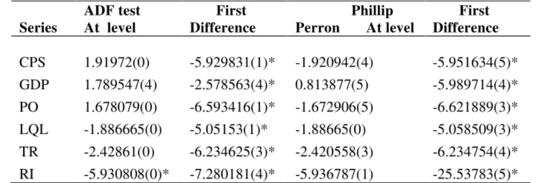
Table 3: Augmented Dickey- Fuller (ADF) Test and Phillips Perron Test for a Unit Root Tests
Series
ADF test At level
First Difference
Phillip Perron At level
First Difference
CPS 1.91972(0) -5.929831(1)* -1.920942(4) -5.951634(5)* GDP 1.789547(4) -2.578563(4)* 0.813877(5) -5.989714(4)* PO 1.678079(0) -6.593416(1)* -1.672906(5) -6.621889(3)* LQL -1.886665(0) -5.05153(1)* -1.88665(0) -5.058509(3)* TR -2.42861(0) -6.234625(3)* -2.420558(3) -6.234754(4)* RI -5.930808(0)* -7.280181(4)* -5.936787(1) -25.53783(5)*
Note * * * indicates the significance level at the 5%, 1% and 10% respectively. Numbers in bracket are the lag length
The estimated results of the Unit root test in table 3 above based on the ADF test, indicates that the null hypothesis of no unit root cannot be rejected at 5% level of significant with the exception of RI, but after taking first differencing all variable are found stationary at 5% level of significant. Thus the confirmatory Philips Perron test also suggests that all series become stationary after taking the first differencing at 5% level of significant.
Bound Test for the long Run Co-integration
Table 4: Critical Values of the Bound Test with Intercept and no Trend
10% level 5% level 1% level
1(0) 1(1) 1(0) 1(1) 1(0) 1(1) 3.247 3.773 3.993 4.533 5.754 6.483
Note** * indicates statistically significant at the 10% 5% and 1% level critical value
The critical values are extracted from Narayan table which comprised both the upper critical values and the lower critical values represented as 1(0) and 1(1) respectively.
Table 5: Estimated F- Test statistics of Joint Significant
GDP= 0.46865
and poverty reduction. However, having long run relationship does not mean causality therefore, to determine whether financial sector development causes economic growth and poverty reduction Unrestricted error correction models were estimated together with Toda and Yamamoto no causality tests. But before estimating the causality relationship the long run coefficient of poverty as a dependent variable is estimated which is presented in table 6 below.
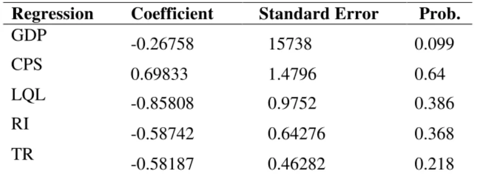
Table 6: Long Run Coefficient Poverty as a Dependent Variable
Regression Coefficient Standard Error Prob.
GDP -0.26758 15738 0.099
CPS 0.69833 1.4796 0.64
LQL -0.85808 0.9752 0.386
RI
-0.58742 0.64276 0.368
TR
-0.58187 0.46282 0.218
Notes * ** *** indicates the significance level at the 1%, 5% and 10% respectively. ARDL(1,0,0,0,0,0,1) selected based on Schwarz Bayesian Criterion
Table 6 above presents the results of the Long run relationship between poverty and Economic growth, financial development, and the instrumental variables of Interest rate and trade percentage of GDP. However, the result indicates that all the explanatory variables are not significantly impacting poverty.
Diagnostic Tests
Test Statistics * LM Version * F Version
A: Serial Correlation CHSQ (1) = 18.5265[.056] F (1, 34) = 26.8344[.056] B: Functional Form CHSQ ( 1) = 0.057956[.810] F (1, 34) = 0.046982[.830] C: Normality CHSQ ( 2) = 1.0613[.588] Not applicable
D: Heteroscadasticity CHSQ ( 1) = 8.0812[.054] F (1, 40) = 9.5300[.054] A: Lagrange multiplier test of residual serial correlation
B: Ramsey’s RESET test using the square of the fitted values
C: Based on a test of skewness and kurtosis of residuals
D: Based on the regression of squared residuals on squared fitted values
Table 7: Short Run Dynamic Vector Error Correction Model
DPOt-1
Dynamic model
DGDPt-1 Dynamic model
DCPSt-1 Dynamic model
DLQLt-1 Model
Variables Coefficient Coefficient Coefficient Coefficient
DGDPt-1 0.34049 0.056878 7.23E-108* 8.25E-10*
(-2.049) (0.25746) (2.3632) (2.4447)
DPOt-1 0.03456 6.3503403 -0.137726 -0.131949
(0.7834) (0.63649) (1.0717) (1.07609)
DLQLt-1 -0.16854 -8.31404348 0.597764
(0.2710) (1.01907) (2.71643)
DCPSt-1 -0.24468 3.845678 0.7113716*
(0.36) (1.345) (3.37778)
DTRt-1 -0.18138 9.9914797 0.296444* 0.251389
(0.137) (1.16402) (2.55193) (2.18389)
DRIt-1 -0.7625 9.361441* 0.12236* -0.026292
(0.402) (1.7911) (1.6182) (0.36604)
ECMt-1 0.058224* 0.18721* 0.570495* 0.208994*
(-0.587) (-2.51151) (-2.4182) (-2.0157)
Note * ** *** indicates the significance level at the 1%, 5% and 10% respectively. ARDL(1,0,0,0,0,0,1) selected based on Schwarz Bayesian Criterion. Numbers in bracket are the t-ratio suggesting the significant of the parameters. Coefficients with ** indicates significant at 5% level.
financial sector development is not enough to trickles down financial resources to the poor other intervening policies accompanied by good governance and equitable income distribution are important.
Figure 1: Stability Test of the Parameters
The diagram above in figure 1 above represents the stability test. Thus the straight lines represents the critical bounds at 5% level of significant the vertical line represents the values of the critical values. However, the figure test the stability of the parameters in the model and based on the results in the figure in table 1 the stability of the model is achieved, since the parallel line do not crossed and is within the 5% level of significant.
Toda-Yamamoto Granger Non- Causality Test Results
Table 8: VAR Granger Causality/Block Exogeneity Wald Test, PO as Dependent Variable
Excluded Chi-sq Prob.
GDP 13.99561 0.2029
CPS 0.683408 0.8771
LQL 1.509796 0.6800
TR 7.048445 0.0704
RI 1.970955 0.5785
All 14.54219 0.4849
Notes * ** *** indicates the significance level at the 1%, 5% and 10% respectively.
Thus, the findings of table 8 to table 13 represents the Toda & Yamamoto no causality tests results. In facts, the result table 8 of the poverty equation with dependent variable PO, the estimated coefficients of GDP, CPS, LQL, TR, RI are not significant indicating that the null hypothesis of no causality cannot be rejected. This indicates that financial sector development and economic growth
Plot of Cumulative Sum of Recursive Residuals
The straight lines represent critical bounds at 5% significance level -5
-10 -15 -20 0 5 10 15 20
have not significantly impact on poverty reduction. The findings of this study do not support the findings of the work of Odhihiambo (2009).
Table 9: VAR Granger Causality/Block Exogeneity Wald Test GDP as a Dependent Variable
Excluded Chi-sq Prob.
PO 2.492726 0.4766
CPS 0.883118 0.8295
LQL 2.363688 0.5004
TR 5.388433 0.1455
RI 1.400474* 0.0054
All 12.41527 0.6474
Note * ** *** indicates the significance level at the 1%, 5% and 10% respectively.
The results of table 9 of the economic growth equation with dependent variable GDP, the estimated coefficients of PO, CPS, LQL, TR, and are not significant. This suggests that poverty reduction, the ratio of bank deposit liabilities to GDP, trade percentage of GDP, do not significantly impact on economic growth. But the coefficient of the RI is statistically significant implies that real interest impact on economic growth.
Table 10: VAR Granger Causality/Block Exogeneity Wald Test CPS as a Dependent Variable
Excluded Chi-sq Prob
PO 0.369909 0.9464
GDP 13.63246* 0.0035
LQL 1.094464 0.7784
TR 3.071064* 0.0058
RI 0.270316* 0.0065
All 14.72064 0.4717
Note* * * indicates the significance level at the 1%, 5% and 10% respectively.
In the credit to private sector equation with dependent variable CPS, in table 10 the estimated coefficient of GDP is significantly positive. This indicates that economic growth is significant with positive value. This implies that economic growth impact on credit to private sector. The coefficients of TR and RI is statistically significant implies that trade percentage of GDP and the real interest rate impact on credit to private sector.
Table 11: VAR Granger Causality/Block Exogeneity Wald Test LQL as a Dependent Variable
Excluded Chi-sq Prob.
PO 4.118325 0.2490
GDP 10.23180* 0.0167
CPS 0.188340 0.9794
TR 9.670154* 0.0216
RI 0.526657 0.9130
All 14.21971 0.4089
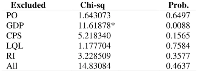
Note * ** *** indicates the significance level at the 1%, 5% and 10% respectively. Table 12: VAR Granger Causality/Block Exogeneity Wald Test TR as a
Dependent Variable
Excluded Chi-sq Prob.
PO 1.643073 0.6497
GDP 11.61878* 0.0088
CPS 5.218340 0.1565
LQL 1.177704 0.7584
RI 3.228509 0.3577
All 14.83084 0.4637
Note* * * indicates the significance level at the 1%, 5% and 10% respectively.
In the trade percentage of GDP equation as provided in table 12, with dependent variable TR, the estimated coefficient of economic growth is significantly positive. This suggests that economic growth significantly positive impact on trade as a percentage of GDP. While in the same estimated equation the coefficients of PO, CPS, LQL, RI, are not significant. Indicating that poverty, credit to private sector, the ratio of banks deposits liabilities to GDP, real interest have not significantly impact on trade percentage of GDP.
Table 13: VAR Granger Causality/Block Exogeneity Wald Test RI as a Dependent Variable
Excluded Chi-sq Prob.
LPO 6.767211 0.0797
LGDP 2.382484 0.4969
LCPS 5.846998 0.1193
LLQL 6.913989 0.0747
LTR 12.42697* 0.0061
All 14.21872 0.5089
In the real interest rate equation with dependent variable RI as presented in table 13 the estimated coefficient of TR is significantly positive. This indicates that trade as a percentage of GDP in Nigeria has a significantly positive impact on real interest rate. The general testing of Toda Yamamoto results support the findings of the studies of Odhianibo (2009), Coccorese (2008), and Odhiambo (2011) which suggest growth led financial sector follow. But do not support the study of Odhihiambo (2009) that financial development and economic growth causes poverty reduction.
5. Conclusion
This study introduces poverty reduction in the competing financial sector economic growth hypothesis in order to investigate whether financial sector development and economic growth contribute towards the eradication of poverty in Nigeria. This study contributes by employing two method of analysis, which includes, the Autoregressive distributed lag model and Toda and Yamamoto approach to no causality. The results suggest that financial sector development and economic growth do not causes poverty reduction in Nigeria. This study provide important understanding that that despite increased in the availability of loan able funds through the financial sector development the poor segment of the Nigerian population does not have access to financial resources. In the case of Nigeria this indicates that financial development alone without equitable income distribution and good governance may not be enough to address the menace of poverty. The finding of this study does not support the work of Odhianibo (2009), who purported to show that financial sector development is positively correlated with poverty reduction. The policy implication here is that financial sector development requires a backup of supporting policies of resources distribution and good governance before, it can pools the mobilized capital into productive investment and equally, channels economic growth to the poor.
References
Adams, A.M. (2012). Financial Openness Induced Growth and Poverty
Reduction. the International Journal of Applied Economics and Finance,
5(1), 75-86.
Adeyemo, A., & Alayande, T. (2003). The Impact of Government Poverty Alleviation on Entrepreneurship Development in Nigeria Readings in Development Policy and Capacity Building in Nigeria: A Book of Readings in Commemoration of the Tenth Anniversary of the Development Policy Centre.
Coccorese, P. (2008). An Investigation on the Causal Relationships Between
Banking Concentration and Economic Growth. International Review of
DFID, (2004). Financial Sector Development: A Pre-requisite for Growth and Poverty Reduction? Policy Division, Department for International Development, London (June).
Dollar, D. & Kraay, A. (2002). Growth is Good for the Poor. J. Econ. Growth, 7,
195-225.
Eggoh, J.C., Bangaké, C. & Rault, C. (2011). Energy Consumption and Economic
Growth Revisited in African Countries. Energy Policy, 39(11), 7408-7421.
Engle, R.F., & Granger, C.W. (1987). Co-Integration and Error Correction:
Representation, Estimation, and Testing. Econometrica: journal of the
Econometric Society, 251-276, Retrieve from
https://students.pomona.edu/2009/zs022009/Desktop/engle1987.pdf
Gelb, A.H. (1989). Financial Policies, Growth, and Efficiency, Policy Planning,
and Research. Working Papers, No. 202 (World Bank). Retrieve
from http://go.worldbank.org/ARQE6SFCT0
Hasan, M. (2011) Democracy and political Islam in Bangladesh, South Asia
Research, 31(2) 97-117.
Jedidi, F.K., & Mensi, S. (2011). The Trade-off between Liberalization Policy and
Financial Crises Dynamics. Asian Social Science, 7(3), 1911-2017.
Johansen, S. (1988). Statistical Analysis of Cointegration Vectors. Journal of
Economic Dynamics and Control, 12(2), 231-254.
Johansen, S. & Juselius, K. (1990). Maximum Likelihood Estimation and Inference on Co-Integration-With Applications to the Demand for Money. Oxford Bulletin of Economics and statistics, 52(2), 169-210.
Kar, M., Nazlıoğlu, Ş. & Ağır, H. (2011). Financial Development and Economic Growth Nexus in the MENA Countries: Bootstrap Panel Granger Causality
Analysis. Economic Modelling, 28(1), 685-693.
King, R.G. & Levine, R. (1993). Finance, Entrepreneurship and Growth. Journal
of monetary economics, 32(3), 513-542.
King, R.G. & Levine, R. (1993a). Finance and growth: Schumpeter might be right The quarterly journal of economics, 108(3), 717-737.
Levine, R. (2005). Finance and Growth: Theory and Evidence. Handbook of
Economic Growth, 1, 865-934.
Lucas Jr,R.E. (1988). On the Mechanics of Economic Development. Journal of
Monetary Economics, 22(1), 3-42.
Maduka, A.C. & Onwuka, K.O. (2013). Financial Market Structure and Economic
Growth: Evidence from Nigeria Data. Asian Economic and Financial
McKinnon, R.I. (1973). Money and Capital in Economic Development, Brookings Institution Press.
Mehran, H. (1998). Financial Sector Development in Sub-Saharan African
Countries, International Monetary Fund.
Mellor, J.W. (1999). Pro-Poor Growth: The Relationship between Growth in
Africa and Poverty Reduction. Abt Associates, Bethesda, MD.
Mery, O.I., Chibuzor, E.E. & Okule, U.D. (2012). Does Financial Sector Development Causes Economic Growth Empirical Evidence from Nigeria. International Journal of Current Research, 4(11), 343-49.
National Bureau of Statistics. (2010). Statistical News: Labor Force Statistics,
No.476. Abuja: The NBS Publication.
Ndebbio, J.E.U. (2004). Financial Deepening, Economic Growth, and
Development: Evidence from Selected Sub-Saharan African Countries Retrieved from http://mpra.ub.uni-muenchen.de/id/eprint/29330
Nnanna, O. (2004). Financial Sector Development and Economic Growth in
Nigeria: An Empirical Investigation. CBN Economic and Financial Review,
42(3).
Nzotta, S. & Okereke, E. (2009). Financial Deepening and Economic
Development of Nigeria: An Empirical Investigation. African Journal of
Accounting, Economics, Finance and Banking Research, Retrieve from http://papers.ssrn.com/sol3/papers.cfm?abstract_id=1534212
Obayelu, O.A. & Awoyemi, T.T. (2012). Spatial Decomposition of Income
Inequality in Rural Nigeria. Journal of Rural Development, 31(3), 271-286.
Odeniran, S.O. & Udeaja, E.A. (2010). Financial Sector Development and
Economic Growth Empirical Evidence from Nigeria. Central Bank of
Nigeria Economic and Financial Review, 48(3), 91-124.
Odhiambo, N.M. (2009). Finance-Growth-Poverty Nexus in South Africa: a
Dynamic Causality Linkage. Journal of Socio-Economics, 38(2), 320-325.
Odhiambo, N.M. (2010). Finance-Investment-Growth Nexus in South Africa: An
ARDL-Bounds Testing Procedure. Economic Change and Restructuring,
43(3), 205-219.
Odhiambo, N.M. (2011). Financial Deepening, Capital Inflows and Economic
Growth Nexus in Tanzania: A Multivariate Model. Journal of Social
Science, 28, 65-71.
Otto, G., Ekine, N.T. & Ukpere, W.I. (2012). Financial Sector Performance and
Economic Growth in Nigeria. African Journal of Business Management
Padhan, P.C. (2007). The Nexus between Stock Market and Economic Activity:
An Empirical Analysis for India. International Journal of Social Economics,
34(10), 741-753.
Pesaran, M.H., Shin, Y. & Smith, R.J. (2001). Bounds Testing Approaches to the
Analysis of Level Relationships, Journal of applied econometrics, 16(3),
289-326.
Pradhan, R.P.P. (2010). The Nexus between Finance, Growth and Poverty in
India: The Cointegration and Causality Approach. Asian Social Science,
6(9), 114.
Ravallion, M. & Datt, G. (2002). Why Has Economic Growth Been More
Pro-Poor in Some States of India than Others?, J. Dev. Econ. 68, 381-400.
Roubini, N. & Sala-i-Martin, X. (1992). Financial Repression and Economic
Growth, Journal of Development economics, 39(1), 5-30.
Saibu, I.M.O., Nwosa, P. & Agbeluyi, A.M. (2011). Financial Development,
Foreign Direct Investment and Economic Growth in Nigeria. Journal of
Emerging Trends in Economics and Management Sciences, 2(2), 146-154.
Schumpeter, J.A. (1911). The Theory of Economic Development. Reprinted 1969,
Oxford: Oxford University Press.
Shan, J. & Morris, A. (2002). Does Financial Development 'Lead' Economic
Growth? International Review of Applied Economics, 16(2), 153-168.
Shaw, E.S. (1973). Financial Deepening in Economic Development, Oxford:
Oxford University Press New York.
Toda, H.Y. & Yamamoto, T. (1995). Statistical Inference in Vector Auto
Regressions with Possibly Integrated Processes. Journal of Econometrics,
66(1), 225-250.
Upchurch, M. (2012). Persistent Economic Divergence and Institutional Dysfunction in Post-Communist Economies: An Alternative Synthesis. Competition & Change, 16(2), 112-129.
World Bank. (1989). World Development Report 1989. New York: Oxford
University Press.
World Bank. (1995). Bangladesh: From Counting the Poor to Making the Poor
Count. Poverty Reduction and Economic Management Network,
Washington: South Asia Division. WorldBank.
Yusuf, M., Malarvizhi, C. & Khin, A.A. (2013), Trade Liberalization Economic
Growth and Poverty Reduction in Nigeria, International Journal of Business