Olumuyiwa A. Lasode
oalasode@yahoo.com Department of Mechanical Engineering University of Ilorin, Ilorin. Nigeria
Mixed Convection Heat Transfer in
Rotating Vertical Elliptic Ducts
This paper presents an investigation into the solution of laminar mixed convective heat transfer in vertical elliptic ducts containing an upward flowing fluid rotating about a parallel axis. The coupled system of normalized conservation equations are solved using a power series expansion in ascending powers of rotational Rayleigh Number, Raτ – a measure of the rate of heating and rotation as the perturbation parameter. The results show the influence of rotational Rayleigh number, Raτ and modified Reynolds number, Rem on the temperature and axial velocity fields. The effect of Prandtl number, Pr, in the range 1 to 5, and eccentricity, e on the peripheral local Nusselt number are also reported. The mean Nusselt number is observed to be highest at duct eccentricity, e=0 for a given Prandtl number. However, results indicate insensitivity of peripheral local Nusselt number to Prandtl number at eccentricity, e=0.866, which is an important result to a designer of rotating vertical heat exchanger. The effect of eccentricity on the friction coefficient is also presented. The parameter space for the overall validity of the results presented is RaτRemPr≤820.
Keywords: mixed convection, rotation, elliptic ducts
Introduction
Research works (Holzworth, 1938; Morris, 1964; Morris, 1965; Morris, 1968; Davies and Morris, 1966; Morton, 1959; Faris and Viskanta, 1969; Tormcej and Nandakumar, 1986) have been carried out to study heat transfer and fluid flow in rotating and non-rotating coolant channels especially of the circular-type geometry while researches (Bello-Ochende, 1985, Bello-Ochende, 1991; Abdel- Wahed, Attia and Hifni, 1984) carried out on elliptic geometry is limited to non-rotating systems. However, recent works (Bello-Ochende and Lasode, 1995; Lasode, 2004) considered rotating elliptic geometry of horizontal orientation.
The power output from electrical machines is to some extent governed by the permissible temperature rise in the insulation surrounding the rotor conductors. Although the forced circulation of air commonly achieves cooling of these conductors over the rotor periphery, there are advantages to be gained if the heat transfer is effected through a suitable coolant flowing inside the conductors themselves especially for large electrical generating machines such as those in Hydro-Electric Power Stations.
Morris (1981) has demonstrated a number of instances in practice where the effect of rotation on the hydrodynamic and thermal characteristics of channel-type flows may have important consequences on the performance of cooling systems of prime movers. He also critically reviewed the assorted literature available on this generalized topic with a view to present it in a form, which bridges the gap between the academic researchers on the one hand, and the eventual industrial user on the other hand.
Morris (1965) conducted an investigation into the influence of rotation on the laminar asymptotic velocity and temperature fields obtained when fluid flows through a vertical tube, which rotates about a parallel axis with uniform angular velocity, subjected to uniform axial temperature gradient. He found out that rotation induced a secondary free convection flow in the plane perpendicular to the axis resulting in non-symmetrical axial velocity and temperature profiles, which modify the resistance to flow and the rate of heat transfer. The conservation equations are solved using a series expansion in ascending powers of the rotational Rayleigh number. 1
Several experimental works have been carried out to confirm the theoretical analyses of the flow process and heat transfer in rotating coolant channels of circular geometry. The earliest reported
Paper accepted December, 2006. Technical Editor: Atila P. Silva Freire.
experimental study was undertaken by Morris (1964), and reported in various forms by Davies and Morris (1965), Morris (1968). These works, which provided data for water and glycerol respectively, were originally undertaken as a study of the performance characteristics of a particular form of rotating closed-loop thermosyphon.
Bello-Ochende (1985) has conducted a numerical study of natural convection in horizontal elliptic cylinders. The method of discretization he proposed allows mesh points to fall on the cylinder boundary so that the problem of irregular boundary is avoided. He presented results for non-uniform heat flux applications at the cylinder periphery in graphical forms for heat transfer and flow regimes for some value of eccentricity and a range of Rayleigh numbers. In another research work, Bello-Ochende (1991) studied the thermal problem of transition-point heat transfer for forced laminar convection in heated horizontal elliptic ducts, using the concept of scale analysis. Results he obtained indicated that in the neighborhood of the eccentricity, e=0.866, optimum results are predicted for the generalized transition-point Nusselt number based on the major diameter and the corresponding generalized thermal entrance length for the parameter space, 0.75≤e<1.0. Abdel-Wahed et al (1984) have done an extensive experimental investigation in the area of laminar developing and fully developed flows and heat transfer in an horizontal elliptic duct. The working fluid was air and two thermal situations were considered; the first was when the duct was having uniform temperature while the other was when the wall temperature was linear. They presented hydrodynamic and thermal results.
Bello-Ochende and Lasode (1995) carried out a parameter perturbation analysis of laminar free and forced convective heat transfer in rotating horizontal elliptic ducts. They investigated the influence of Prandtl number and eccentricity on axial velocity and temperature profiles. They also studied the effect of Prandtl number and eccentricity on mean Nusselt number. Results they obtained indicated optimum heat transfer at duct eccentricity, e=0.433.
Morton (1959) did a wonderful job in his study of buoyancy force due to the earth’s gravitational field but with geometry of e=0 and a stationary tube. Morton presented radial temperature distribution, axial velocity and streamfunction, all in power series.
transfer a critical aspect ratio of 0.50 (e=0.866) is predicted and that perturbation results indicate a considerable effect of inclination on circular ducts and elliptic geometry of e=0.433 while the effect is negligible for the configuration for e=0.866.
Faris and Viskanta (1969) studied laminar combined forced and free convection heat transfer in a horizontal tube using a perturbation method. They presented approximate analytical solutions as well as average Nusselt numbers graphically for a range of Prandtl and Grashof numbers. Tormcej and Nandakumar (1986) studied mixed convective flow of a power law fluid in horizontal ducts. Lasode (2004) used parameter perturbation technique for the analysis of laminar free and forced convection in rotating horizontal elliptic cylinders.
The present study is an investigation of mixed convective heat transfer for upward flowing fluid in vertical elliptic ducts rotating about a parallel axis. A physical model for the solution of the problem is shown in Fig. 1. Particular attention is paid to the fully developed flow regime in this study where the temperature and axial velocity are far ahead of axial locations along the ducts where entry effects could be felt. The governing equations of continuity, momentum and energy transfer are solved using single parameter perturbation technique. The technique is an approximate analytic method in which the normalized axial velocity, temperature and cross-flow stream function are expanded in power series using the rotational Rayleigh number, Raτ, as the perturbation parameter. For the elliptic tubes considered, a boundary coordinate,ξ, is developed from the parametric equations of an ellipse for the solution of the normalized governing equations to be valid at any boundary location, for the Dirichlet problem.
Nomenclature
a,b = Semi – major and semi – minor axes respectively Cfr = Friction coefficient
Cp = Specific heat at constant pressure e = Eccentricity.
F (r,θ) = A function specifying the temperature distribution in the (r, θ)-plane
g = Acceleration due to gravity Gaτ = Gravitational Rayleigh number
H = Distance between the axis of rotation and tube axis i = Order of perturbation solution
K = Thermal conductivity of the fluid
Nu (θ),Num = Peripheral local and mean Nusselt number respectively
O = Tube axis.
O’ = Centre of the fixed frame of reference
p,P = Elemental fluid and pressure distribution respectively P(r,θ) = A function specifying the pressure distribution in the
(r,θ) – plane Pr = Prandtl number, u/a.
r, rb = Any radial distance from centre and to boundary, respectively
R = Dimensionless radius Raτ = Rotational Rayleigh number Rem = Modified Reynolds number Ro* = Rossby number
T, Tb = Dimensional local and dimensional bulk temperature respectively
Tw = Wall temperature
u ,v, w = Dimensional velocity in the radial, azimuthal and axial directions respectively
W, Z = Dimensionless axial velocity and distance in the z-direction respectively
Greek Symbol α = Thermal diffusivity
β = Coefficient of thermal expansion
Ω = Angular velocity of tube
ρ = Density of fluid
ξ = Boundary coordinate
λ Angle between normal to the tangent and the horizontal
εa = Axes displacement parameter
η,ηb = Dimensionless local and dimensionless bulk temperatures respectively
µυ = Dynamic and kinematic viscosities respectively
θ = Angle in degrees
στ = Axial pressure and temperature gradients respectively
ψ = Streamfunction
χ(θ) = A form of the boundary coordinate, ξ ∇2 = Laplace operator
∇4
= Bi-harmonic operator
Physical Problem and Mathematical Formulations
The physical model and the cylindrical polar coordinate (r,θ,z) system are shown in Fig.1
For the flow condition, the following assumptions should be noted.
• Flow is laminar and fully developed.
• The elliptic duct is vertical and rotates in the parallel mode.
• Heated tube is treated and the thermal conductivity of the tube material is high enough to smooth out circumferential variation in wall temperature.
• The fluid temperature distribution can be mathematically stated as,
z T
Tw= 0+τ . (1)
due to the combined assumption of fully developed flow and uniform axial heating. Equation (1) is applicable at the tube wall meaning that the wall temperature will increase uniformly in the direction of flow. At any axial location the difference in the wall temperature, Tw, and any local value of temperature in the flow will also be functionally related to the axial temperature gradient.
• With the exception of density, the fluid properties are taken to be constant with temperature.
Because distances well away from inlet influences are being considered, the pressure distribution is constrained to be of the form
( )
θ γz pr,P= + . (2)
• It is assumed that there are no chemical reactions, no heat sources within the fluid, radiation is neglected and viscous dissipation is ignored.
The following non–dimesionalization parameters are adopted for the dependent and independent variables:
= − =
− = = =
r r , r
aP T T ; w W ; a z ; a r R
r w
δ δψ µ µ δ δψ υ ν
τ η υ
Figure 1. Physical model, coordinate axes and regions of the ducts.
The normalized governing equations are as follows:
Normalized Streamfunction Equation
(
)
(
)
(
)
(
)
01 1
1 2
4
= ∂ ∂ +
∂ ∂ ∈ +
+
∂ ∂ + ∂ ∂ +
∂ ∇ ∂ + ∇
∗
θ ψ η θ
η
θ η θ θ η θ
ψ ψ ψ
τ τ
τ
, R
, R Re
Ro Ra Ra
sin R Cos R Ra , R , R
m a
. (4)
Where,
( )
ψψ 2 2
4 =∇ ∇
∇ . (5)
The Equation (5) above is a Biharmonic Operator.
Normalized Axial Velocity Equation
(
)
(
)
4 01
2
= − + ∂ ∂ +
∇ η
θ ψ
m Re ,
R W , R
W . (6)
Normalized Energy Transport Equation
(
)
(
)
02 + =
∂ ∂ +
∇ W
, R
, R Pr
θ η ψ
η (7)
The normalization procedure adopted highlights the following dimensionless groups, which parametrically govern this problem.
αυ βτ Ω
τ
4 2H a
Ra = Rotational Rayleigh Number
z v a Rem
∂ ∂ −
= ρ
ρ 2
4 3
Modified Reynolds Number
z v H
a Ro
∂ ∂ =
∗ ρ
ρ Ω
2
2
Rossby Number
αυ τ β
τ
4
a g
Ga = Gravitational Rayleigh Number
H a a =
ε Axis displacement parameter
α υ =
Pr Prandtl Number
The rotational Rayleigh number, Raτ emerges from the
centripetal buoyancy terms in the momentum equations. This is similar to the Rayleigh number encountered by Morton (1959) in the study of buoyancy force due to the earth’s gravitational field but with the gravitational acceleration replaced by the centripetal acceleration measured at the center line. The Rossby number, Ro* has its origin in the coriolis acceleration terms. The modified Reynolds number, Rem approximates to the usual through-flow Reynolds number when the buoyancy effects are not included.
Solution Technique
The normalized governing equations are solved using a series expansion in ascending powers of the rotational Rayleigh number, Raτ. This asymptotic series expansion is truncated at the
second-order, and therefore presents an approximate solution. This technique was successfully used by Morton (1959); Morris (1965) as well as Bello-Ochende and Lasode (1995). The need for the satisfaction of the boundary conditions for different polar coordinates at the boundary of the ellipse requires the consideration of the eccentricity, e, and the angular position, θ. For the derivation of the boundary coordinate, ξ, the parametric equations of an ellipse are invoked and is given as,
(
)
(
θ)
ξ 2 2
2
1 1
cos e
e −
−
= (8)
Boundary Conditions
The normalized boundary constrains are as follows:
(i) ψ,W y and η are zero when R= ξ , that is, at the boundary.
(ii) ψ,Wand η are finite at R = 0, that is at the core of the duct.
(iii)
θ ψ ψ
∂ ∂ ∂ ∂
R , R
1
are zero at R= ξ , but finite at the centre of
the elliptic duct.
The parameter perturbation technique adopted in the solution of the problem gave rise to the power series representation of the normalized governing equations which is expanded with rotational Rayleigh Number, Raτ, as follows:
(i) Stream function
... Ra Ra
Ra i i
n i
i
+ + + = ∑ =
= 2
2 0
0
ψ ψ ψ ψ
ψ τ τ τ (9)
(ii) Axial Velocity
... W Ra W Ra W W Ra
W n i i
i i
+ + + = ∑ =
= 2
2 0
0 τ τ τ
(10)
(iii) Temperature Field
... Ra Ra
Ra i i
n i
i
+ + + = ∑ =
= 2
2 0
0
η η η η
Substituting Eqs. (9), (10) and (11) into Eqs. (4), (6) and (7) respectively, it is possible upon integrating the resulting cascade of differential equations and application of the boundary constraints, to arrive at the following solutions:
Zeroth-Order Solutions
(i) Zeroth–order Streamfunction
0
0=
ψ (12)
There can be no flow in the (r,θ) – plane when Raτ=0, due to the absence of circulation or secondary flow. This corresponds to a no-heating condition.
(ii) Zeroth–order Axial Velocity
(
R)
RemW0= ξ− 2 (13)
(iii) Zeroth order Temperature
(
2 2 4)
0 3 4
16 R R
Rem
+ −
= ξ ξ
η (14)
First-Order Solutions
(i) First-order Streamfunction
(
3 2 2 4 6)
1 10 21 12
4608 R R R R
sin
Rem − + −
= θ ξ ξ ξ
ψ (15)
(ii) First-order Axial Velocity
[
6 4 2 2 3]
6 4 2 2 3 2 5 2 1 19 27 9 576 19 51 49 10 843 1 ξ ξ ξ ξ ξ ξ ξ θ τ − + − + + − − + − × = R R R Ra Re R R R R R . cos Re W m m (16)
(iii) First-order Temperature
(
)
(
)
(
)
(
)
(
)
(
)
[
4 3 2 2 4 6 8]
4 11 9 7 2 5 2 3 4 5 2 1 16 108 304 211 10 686 3 10 1 210 30 1125 175 2600 500 3000 735 1325 381 22118400 R R R R Ra . Re Ga R Pr R Pr R Pr R Pr R Pr R Pr cos Re m m + − + − × − + − + + + − − + + + − + = ξ ξ ξ ξ ξ ξ ξ ξ ξ θ η τ τ (17) Second-Order Solutions
(i) Second-order Streamfunction
The final solution contain numerical coefficients of an unwieldy nature, therefore they have been grouped within summations signs and actual values tabulated in Table 1 below.
( ) ( )
(
)
( ) ( ) ( ) ( )(
)
(
)
(
( ))
( )(
)
∑ − ∑ + ∑ + + ∑ + +∑ + = = + − + = + − + ∗ = + − + + = − = − − − − 6 0 1 2 5 1 2 7 6 0 1 2 6 1 2 4 7 0 1 2 7 1 2 1 2 7 2 2 1 2 7 73 2 2
1 2 2 1 7 1 2 1 2 2 10 424 4 10 843 1 10 21 2 4608 2 u u u u m t t t t m s s s s s m r r r
r r r
r r r r m R C Ra x . sin Re Ga R C x . cos Re Ro R Pr D C x . sin a Re R Pr D C R Pr D C sin Re ξ θ ξ θ ξ θ ε ξ ξ θ ψ τ τ (18)
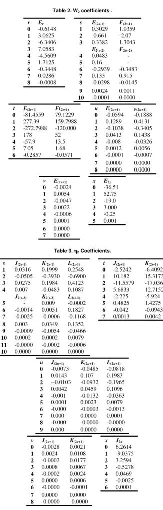
(ii) Second-order Axial Velocity (see Table 2 below for actual values of coefficients)
( ) ( ) ( )
(
)
( ) ( ) ( )(
)
( ) ( ) ( ) ( )(
)
( ) ( ) ( ) ( )(
)
( ) ( ) ( )(
)
( ) ( ) ( )(
)
( ) ( ) ∑ − ∑ + ∑ + − ∑ + + ∑ + +∑ + + ∑ = = − = + − + = + − + + = + − + + − − − − − − − − − − = − 5 0 2 5 2 4 2 7 0 1 2 7 1 2 2 8 0 1 2 8 1 2 1 2 7 3 6 0 1 2 1 6 1 2 1 2 7 2 3 1 10 4 2 2 10 2 2 2 2 1 2 2 17 1 2 1 2 7 3 8 0 2 8 2 3 10 686 3 9216 10 106 1 10 123 2 10 123 2 2 4608 2 x x x x m v v v v m * u u u u u a m t t t t m s s s s s s s s s s m r r r r m R E Ra x . Re Ga R E sin Re Ro R Pr F E Ra x . cos Re R Pr F E Ra x . cos Re Ga R Pr F E R Pr F E x . cos Re R E Re W ξ ξ θ ξ θ ε ξ θ ξ ξ θ ξ τ τ τ τ τ (19)(iii) Second-order Temperature (see Table 3 below for actual values of coefficients)
(
)
( ) ( ) ( )(
)
( ) ( ) ( ) ( )(
)
( ) ( ) ( ) ( )(
)
( ) ( ) ( ) ( ) ( )(
)
( ) ( ) ( ) ( )(
)
( ) ( ) ( ) ∑ × ∑ + × ∑ + + × − ∑ + × + ∑ + + + ∑ + + × + ∑ + + × = = − = + − + + = + − + + + = + − + + = − − − − − = − − − − − = − 6 0 2 6 2 2 4 2 2 8 0 1 2 8 1 2 1 2 4 2 9 0 1 2 9 2 1 2 1 2 1 2 7 3 7 0 1 1 2 7 1 2 1 2 2 7 2 2 12 5 3 2 12 2 3 2 3 2 3 2 4 1 3 2 19 2 1 2 1 2 1 2 7 3 9 0 2 9 2 2 2 2 7 2 10 686 3 10 373 7 10 123 2 10 123 2 10 123 2 2 10 123 2 3 x x x x m v v v v v m * u u u u u u a m t t t t m s s s s s s s s s s s s m r r r r r r m R J Ra . Re Ga R Pr K J . sin Re Ro R Pr L Pr K J . cos Re R Pr K J Ra . cos Re Ga R Pr L Pr K J R Pr L Pr K J . cos Re R Pr L K J . Re ξ ξ θ ξ θ ε ξ θ ξ ξ θ ξ η τ τ τ τ (20)The overall validity range for the solution presented is obtained by the continuation procedure suggested by Tormcej and Nandakumar (1986) in which the bisection method is incorporated.
Table 1. ψψψψ2 Coefficients.
s C(2s+1) D(2s+1) r C(2r-1) D(2r-1)
0 1.0315 3.3052 1 1.3223 4.1400
1 -2.4913 -8.1719 2 -2.0294 -7.826
2 1.9842 6.9006 C2r D2r
3 -0.6380 -2.6040 3 0.1097 5.3864
4 0.1302 0.6770 4 0.9581 -2.2647
5 -0.0182 -0.01172 5 -0.3925 0.5195
6 0.0015 0.0104 6 0.0312 -0.0545
7 0.0000 0.0003 7 -0.0015 0.0017
t C(2t+1) u C(2u+1)
0 0.0432 0 2986.08
1 -0.1125 1 -6365.03
2 0.1042 2 3800
3 -0.0451 3 -450
4 0.0117 4 30
5 -0.0015 5 -1
Table 2. W2 coefficients .
r Er s E(2s-1) F(2s-1)
0 -0.6148 1 0.3029 1.0359
1 3.0625 2 -0.661 -2.07
2 -6.3406 3 0.3382 1.3043
3 7.0583 E2(s-2) F2(s-2)
4 -4.5609 4 0.0483 -
5 1.7125 5 0.16 -
6 -0.3448 6 -0.2939 -0.3483
7 0.0286 7 0.133 0.915
8 -0.0008 8 -0.0298 -0.0145
9 0.0024 0.0011
10 -0.0001 0.0000
t E(2t+1) F(2t+1) u E(2u+1) F(2u+1)
0 -81.4559 79.1229 0 -0.0594 -0.1888
1 277.39 159.7988 1 0.1289 0.4131
2 -272.7988 -120.000 2 -0.1038 -0.3405
3 178 52 3 0.0413 0.1438
4 -57.9 13.5 4 -0.008 -0.0326
5 7.05 1.68 5 0.0012 0.0056
6 -0.2857 -0.0571 6 -0.0001 -0.0007
7 0.0000 0.0000
8 0.0000 0.0000
v E(2v+1) x E2x
0 -0.0024 0 -36.51
1 0.0054 1 52.75
2 -0.0047 2 -19.0
3 0.0022 3 3.000
4 -0.0006 4 -0.25
5 0.0001 5 0.001
6 0.0000
7 0.0000
Table 3. ηηηη2 Coefficients.
s J(2s-1) K(2s-1) L(2s-1) t J(2t+1) K(2t+1)
1 0.0316 0.1999 0.2548 0 -2.5242 -6.4092
2 -0.0505 -0.3930 -0.6900 1 10.182 15.3173
3 0.0275 0.1984 0.4123 2 -11.5579 -17.036
4 0.007 -0.0483 0.1087 3 5.6833 12.7152
J2(s-3) K2(s-3) L2(s-3) 4 -2.225 -5.924
5 - 0.009 -0.0002 5 0.4825 1.4275
6 -0.0014 0.0051 0.1827 6 -0.042 -0.0943
7 -0.0025 -0.0006 -0.1168 7 0/0013 0.0042
8 0.003 0.0349 0.1352
9 -0.0009 -0.0054 -0.0466
10 0.0002 0.0002 0.0079
11 -0.0000 -0.0002 -0.0006
10 0.0000 0.0000 0.0000
u J(2u+1) K(2u+1) L(2u+1)
0 -0.0073 -0.0485 -0.0818
1 0.0143 0.107 0.1983
2 --0.0103 -0.0932 -0.1965
3 0.0042 0.0459 0.1096
4 -0.001 -0.0132 -0.0363
5 0.0001 0.0023 0.0079
6 -0.000 -0.0003 -0.0013
7 0.000 0.0000 0.0001
8 -0.000 -0.0000 -0.0000
9 0.000 0.0000 0.0000
v J(2v+1) K(2v+1) x J2x
0 -0.0028 0.0021 0 6.2614
1 0.0024 0.0108 1 -9.0375
2 -0.0002 0.0177 2 3.2594
3 0.0008 0.0067 3 -0.5278
4 -0.0002 0.0024 4 0.0469
5 0.0000 0.0006 5 -0.0025
6 -0.0000 -0.0001 6 0.0001
7 0.0000 0.0000
8 -0.0000 -0.0000
Peripheral Local Nusselt Number
The Nusselt number is a dimensionless quantity indicative of the rate of energy convection from the surface. For the conduction referenced heat transfer with respect to the bulk temperature and considering the normal temperature gradient, we have the peripheral local Nusselt number, Nu (θ), as,
( )
θ η η ( )θ(
λ−θ)
∂ ∂
= = cos
R
Nu R x
b 2
(21)
where,
(
) (
)
( )
(
) (
)
( ) ∫ ∫ ∫ ∫ = πχ θ
πχ θ
θ θ θ η
θ θ θ η
η 2
0 0 2
0 0
RdRd , R W , R
RdRd , R W , R
b (22)
and
( )
θ ξχ = (23)
Mean Nusselt Number
The mean Nusselt Number is obtained from,
( )
θ θ ππ
d Nu Num = 2∫
0
2 1
(24)
The trapezoidal rule was used to evaluate Eq. (24) above.
Friction Coefficient
The normalized form of the friction coefficient (the parameter indicating the influence of rotation on the established resistance to flow using the Blasius friction factor) is given by:
(
)
( ) 2
2
0 0 2 2
1 4
∫ ∫ − =
πχ θ
θ π
WRdRd Re e r
Cf m (25)
Discussion of Results
Figures 2a and 2b present the typical illustrations of temperature and axial velocity perturbation components respectively, along the major diameter for e=0.433.
a) Temperature
b) Axial Velocity
Figure 2. (Continued).
The zeroth-order component is parabolic, and it is the one usually encountered in pure forced convective flows. The first- and second-order perturbation components are sinusoidal in nature. The resultant shows the effects of the first- and second-order components on the zeroth-order component. The sinusoidal nature of the first- and second-order perturbation components account for the shift in the maximum local values of the temperature and axial velocity profiles.
The effects of rotational Rayleigh number, Raτ, on the temperature and axial velocity distributions can also be noticed. The tendency for the warmer and less dense fluid to move towards the outer region of the tube’s cross-section under the influence of centripetal buoyancy is clearly shown. The centrifugal buoyancy is what is really responsible for the distortion of the temperature and axial velocity profiles. At the maximum local temperature value, the contributions of the zeroth-order, first-order and second-order are 99.23%, 0.41% and 0.36% respectively while at the maximum axial velocity value; the contributions are 99.72%, 0.25%, and 0.03% respectively. Considering the rigour involved in obtaining the second-order coefficients and its percentage contribution to the entire solution, obtaining higher order terms may not significantly alter the accuracy of the results.
However, the first- and second-order perturbation components are insignificantly small when computed along the minor diameter, and only the zeroth-order components contribute to the axial velocity and temperature distributions.
Figures 3a and 3b present the typical effect of eccentricity on the temperature and axial velocity profiles respectively along the minor diameter. The results show a sudden collapse of the maximum local value of temperature at e=0.866, almost flattens out, compared to the corresponding axial velocity profile. Moreover, it can be noticed that the axial velocity profile shows less drastic response to increase in eccentricity than the temperature field. While maximum local temperature at e=0.866 collapses to 7.1% of the corresponding local maximum value at e=0, the maximum local value of the axial velocity at e=0.866 collapses to 33.3% of the corresponding local maximum value at e=0.
a) Temperature
b) Axial Velocity
Figure 3. Effect of Eccentricity on temperature and axial velocity distributions along the minor diameter. (Raττττ=10, Rem=50, Pr=1, Ro*=1,
εεεεa=1/48, Gaττττ=1).
Figures 4a and 4b present the effect of Prandtl number, Pr, on the temperature and axial velocity profiles respectively for the range of parameter shown. The results show that increase in Prandtl number, Pr, manifests in a marked shift of the temperature profile away from the origin and marginal increase in the maximum local value while the axial velocity profile shows no observable response. This shows that axial velocity profiles are insensitive to Prandtl number in the range of Prandtl number considered, that is, Pr = 1 to 5. This may be attributable to the influence of opposing gravitational field on the upward flowing fluid.
a) Temperature
b) Axial Velocity
Figure 4. (Continued).
Figures 5a and 5b show the effect of rotational Rayleigh number, Raτ, on the temperature and axial velocity profiles respectively along the major diameter for solutions up to the second order for duct eccentricity, e=0.433. Increase in the rotational Rayleigh number, Raτ, which is the measure of heating and rotation, results in the gradual shift of the points of maximum value of the local temperature away from the origin and pronounced increase in the maximum value. The secondary flow (convective flow induced due to rotation) increases correspondingly and the temperature profiles become distinctly different from those of pure forced convection. Figure 5b indicates that as the rotational Rayleigh Number, Raτ, increases, the deformation of the axial velocity and its deviation from the parabolic nature for no-heating condition is marginal. This may also be attributable to the opposing gravitational field.
a) Temperature
b) Axial Velocity
Figure 5. Effect of rotational Rayleigh number on temperature and axial velocity distributions (Rem=20, Pr=1, Ro*=1, εεεεa,=1/48, e=0.433, Gaττττ=1).
Figures 6a and 6b show the effect of modified Reynolds number, Rem on the temperature and axial velocity profiles respectively, along the major diameter up to the second-order solution for an elliptic tube of eccentricity, e=0.433 respectively. The general lateral shifts in the temperature and axial velocity profiles away from the origin, due to the influence of heating and rotation are noticeable. There are corresponding increases in the maximum values of the local temperature and axial velocity as the modified Reynolds number increases.
a) Temperature
b) Axial Velocity
Figure 6. Effect of modified Reynolds number on temperature and axial velocity distributions (Raττττ=10, Pr=1, Ro*=1, εεεεa=1/48, e=0.433, Gaττττ=1).
a) Rotational Rayleigh number, Raτ = 5
b) Rotational Rayleigh Number, Raτ = 10
Figure 7. Effect of eccentricity on local Nusselt number (Rem=50, Pr=1, Ro*=1, εεεεa=1/48, Gaττττ=1).
Figures 8a and 8b show the plot of mean Nusselt number against duct eccentricity at rotational Rayleigh number, Raτ=5 and Raτ=10
respectively. Figure 8a indicates that mean Nusselt number is invariant with eccentricity up to e=0.433, beyond which it drops sharply. However, for Raτ=10 (Fig. 8b), mean Nusselt number
monotonically decreases with eccentricity with a change to higher gradient of decrease noticeable at e=0.6. The optimum heat transfer seems to be at e=0. The values of mean Nusselt number is higher for Raτ=10 than for Raτ=5 for each elliptic geometry considered. This
result is different from that of Bello- Ochende and Lasode (1995) in which optimum heat transfer was indicated at e=0.433 for the horizontal configuration they considered. The difference can be attributed to the effect of gravitational buoyancy included in this analysis.
a) Rotational Rayleigh Number, Raτ=5
Figure 8. Effect of eccentricity on mean Nusselt number (Rem=50, Pr=1,
Ro*=1, εεεεa=1/48, Gaττττ=1). Effect of eccentricity on mean Nusselt number (Re =50, Pr=1, Ro*
=1, εεεε=1/48, Ga=1).
b) Rotational Rayleigh Number, Raτ=10
Figure 8. (Continued).
Figures 9a, 9b and 9c show the effect of Prandtl number, Pr, on the peripheral local Nusselt number for elliptic ducts of e=0, e=0.433 and e=0.866 respectively. Figure 9a (e=0) shows reductions in peripheral local Nusselt number for all angular positions between 0ºand 360º, where the maximum value occurs for the range of Prandtl number, Pr, considered (that is, Pr = 1 to 5). Figures 9b (e=0.433) and 9c (e=0.866) show a form of cosinusoidal variation of peripheral local Nusselt number with angular positions for the range of Prandtl number, Pr, under consideration. Moreover, Fig. 9c (e=0.866) reveals that the peripheral local Nusselt number seem to be insensitive to changes in the Prandtl number, Pr. This may be an important result for designer of rotating vertical elliptic heat exchanger who would like to use any available fluid as the heat transfer fluid since the Prandtl Number is a fluid property.
a) Eccentricity, e=0
b) Eccentricity, e=0.433
Figure 9. Effect of Prandtl number on local Nusselt number (Raττττ=5, Rem=30, Ro
*
c) Eccentricity, e=0.866
Figure 9. (Continued).
Figures 10a and 10b show the effect of modified Reynolds number and eccentricity on friction coefficient respectively. From Fig. 10a, it is seen that the increase in modified Reynolds number results to a decrease in friction coefficient and that the geometry of the duct has a pronounced effect on the friction coefficient. Figure 10b shows the plot of friction coefficient against the tube eccentricity for heating, at Raτ=5 and Raτ=10, conditions. The result
indicates monotonic increase in friction coefficient for both conditions. For the elliptic ducts, the numerical values of the friction coefficient for Raτ=10 is lower compared to the values for Raτ=5
showing that heating and rotation reduce friction coefficient, though the two curves seems to merge.
Figure 10a. Effect of modified Reynolds number on friction coefficient at various eccentricity (Raττττ=5, Pr=1, Ro
*
=1, εεεεa=1/48, Gaττττ=1).
Eccentricity, e
Figure 10b. Effect of eccentricity on friction coefficient at various rotational Rayleigh number(Rem=50, Pr=1, Ro
*
=1, εεεεa=1/48, Gaττττ=1).
Conclusion
This analysis is valid for low values of rotational Rayleigh number, Raτ. At the fully developed flow region considered, it is
shown that for rotating vertical elliptic ducts, the axial velocity and temperature profiles as well as Nusselt number and friction coefficient are functions of rotational Rayleigh number, Raτ,
modified Reynolds number, Rem, and Prandtl number, Pr.
The results show that, for a vertical elliptic duct with upward flowing fluid rotating about a parallel axis, the perturbation parameter, Raτ, is responsible for the lateral shift of the temperature
and axial velocity profile away from the origin along the major diameter and its deviation from the usual parabolic profile associated with pure forced convection due to secondary flow effects and buoyancy forces. Along the minor diameter, these effects are insignificant. Axial velocity profiles are insensitive to rotational Rayleigh number, Rat and Prandtl number, Pr, changes along the major diameter. Modified Reynolds number increases manifest in increases in the maximum value of temperature and axial velocity profiles. The results also predict that the peripheral local Nusselt number is insensitive to Prandtl number changes for duct eccentricity, e=0.866. This is an important result for a designer of rotating vertical elliptic heat exchanger. For vertical elliptic ducts rotating about a parallel axis, mean Nusselt number is invariant with eccentricity up to e=0.433 for low rates of heating and rotation, and monotonically decreases with eccentricity for high heating rates. Optimum heat transfer is experienced at duct eccentricity, e=0 (circular duct).
The result is in agreement with the published works of Morris (1981) and Morris (1965) for rotating circular ducts.
References
Abdel- Wahed, R.M., Attia, A.E., and Hifni, M.A., 1984, “Experiments on Laminar flow and heat transfer in as elliptic duct”, International Journal of Heat and Mass transfer, Vol.27, No.12, pp. 2397 – 2411.
Adegun, I.K., 1992, “Analytical study of convective heat transfer in inclined elliptic ducts”, M. Eng. Thesis, University of Ilorin, Ilorin, Nigeria. Bello-Ochende, F.L and Layside, O.A., 1995, ”Convective Heat transfer in Horizontal elliptic ducts in Parallel Mode Rotation”, International Journal of Heat and Technology, Vol.3, No. 1, pp. 105-122.
Bello – Ochende, F.L., 1985, “A numerical study of Natural convection in horizontal elliptic cylinders”, Revista Brasileira de Ciencias Mecanicas, Vol.VII, No. 4, pp. 353 – 371.
Bello – Ochende, F. L., 1991, “Scale Analysis of Entrance Region Heat transfer for forced convection in elliptic cylinders”, Proceedings of the 11th ABCM Mechanical Engineering Conference, Sao Paulo, SP- Brazil.
Davies, T.H., and Morris, W.D., 1966, “Heat transfer characteristics of a closed loop rotating thermosyphon”, Proceeding of the 3rd International Heat Transfer Conference, American Institute of Chemical Engineers, Chicago, USA, Vol.2, pp. 172.
Faris, G.N., and Viskanta, R., 1969, “An analysis of laminar combined forced and free convective heat transfer in a horizontal tube”, International Journal of Heat and Mass Transfer, Vol.12, pp 1295 – 1309.
Holzworth. H., 1938, “Die Entwicklung der Holzworth - Gas Turbine, Holzworth – Gas turbinen”, G.m.b.H. Muehlmeim – Ruhr.
Lasode, O. A., 2004, “Perturbation solution to mixed convection in rotating horizontal elliptic cylinders”, AIAA Journal of Thermophysics and Heat Transfer, Vol.18, No.1, pp.79-86.
Morris, W.D., 1964, “Heat transfer characteristics of a rotating thermosyphon”, PhD Thesis, University of Wales, Swansea.
Morris, W.D., 1965, “Laminar Convection in a heated vertical tube rotating about a parallel axis”, Journal of Fluid Mechanics, Vol.21, Part 3, pp. 453 – 464.
Morris, W.D., 1968, “Terminal Laminar convection in uniformly heated rectangular duct”, Thermo and Fluid Mechanics convention, I. Mech. E., Bristol, Paper No. 4.
Morton, B. R., 1959, “Laminar convection in uniformly heated horizontal pipes at low Rayleigh Number”, Quarterly Journal of Mechanics and Applied Mathematics, Vol.XII, pp. 411 – 420.