Tax revenue reforms and income distribution in developing countries

(1)

REM WORKING PAPER SERIES

Tax Revenue Reforms and Income Distribution in Developing

Countries

Sanjeev Gupta, João Tovar Jalles

REM Working Paper 0137-2020

July 2020

REM – Research in Economics and Mathematics

Rua Miguel Lúpi 20, 1249-078 Lisboa,

Portugal

ISSN 2184-108X

Any opinions expressed are those of the authors and not those of REM. Short, up to two paragraphs can be cited provided that full credit is given to the authors.

(2)

REM – Research in Economics and Mathematics

Rua Miguel Lupi, 20 1249-078 LISBOA Portugal Telephone: +351 - 213 925 912 E-mail: rem@iseg.ulisboa.pt https://rem.rc.iseg.ulisboa.pt/ https://twitter.com/ResearchRem https://www.linkedin.com/company/researchrem/ https://www.facebook.com/researchrem/

(3)

1

Tax Revenue Reforms and Income

Distribution in Developing Countries*

Sanjeev Gupta

$

_{João Tovar Jalles}

#

June 2020

Abstract

We explore the impact of major revenue mobilization episodes on income distribution dynamics using a new “narrative” database of major policy changes in tax and revenue administration systems, covering 45 emerging and low-income countries from 2000 to 2015. Our main finding is that after a tax reform (particularly those affecting the personal income or the operation of the revenue administration), the Gini index falls and the bottom income share rises. This result does not hold for sub-Saharan Africa, calling into question the design of tax reforms implemented in the region (mostly fragile states in the sample). In general, to reduce more rapidly income inequality (and improve the income prospects of the poorest strata of the population), it would be more effective to implement tax reforms when the economy is growing relatively slowly. Finally, the smaller the government and the smaller the tax system, the larger the beneficial impact of tax reforms on income distribution. Our results are robust to a battery of sensitivity and robustness tests.

JEL: C33, C36, D63, E32, E62, H20

Keywords: income distribution; Gini; fiscal policy; impulse response functions; endogeneity;

nonlinearities; government size

*_{This work was supported by the Bill and Melinda Gates Foundation. Mr. Jalles also acknowledges support from the}

FCT (Fundação para a Ciência e a Tecnologia) [grant numbers UID/ECO/00436/2019 and UID/SOC/04521/2019]. The authors are grateful to Benedict Clements and Mark Plant for very helpful suggestions on an earlier draft. A shorter version was issued as a Center for Global Development paper (CGD Policy Paper 175, June 2020). Any remaining errors are the authors’ sole responsibility. The usual disclaimer applies.

$_{Center for Global Development. 2055 L St NW, Washington, DC 20036, United States. email:}_{sgupta@cgdev.org} #_{ISEG, University of Lisbon. REM/UECE. Rua Miguel Lupi 20, 1249-078 Lisbon, Portugal. Centre for Globalization}

and Governance and Economics for Policy, Nova School of Business and Economics, Rua Holanda 1, 2775-405 Carcavelos, Portugal. email: joaojalles@gmail.com.

(4)

2

1. Introduction

There is considerable emphasis on both emerging and low-income countries collecting more taxes from domestic sources to help achieve the Sustainable Development Goals (SDGs). This is because the resources required to finance the SDGs are huge and the ability of advanced countries to transfer resources through aid are heavily constrained by their debt-to-GDP ratio, which now exceeds 100 percent of GDP on average and are likely to increase even further following the COVID-19 crisis. The Addis Ababa Agenda for financing development pays special attention to domestic resource mobilization in emerging and low-income countries and SDG 17.1 tracks country level domestic resource mobilization efforts. However, domestic resource mobilization should not come at the cost of impoverishment of the poor or widening of income disparities.

Developing countries are on pace to collect public revenues of about $4,444 per person annually by the end of 2020, which corresponds to over $1 per person per day. This compares with $16,200 per person in richer countries (2015 data). If developing countries were to improve revenue-to-GDP by an extra 2 percentage points by the end of 2020, their annual public revenues would increase collectively by $144bn – which corresponds to more than the total amount of development aid recorded in 2016 (Oxfam, 2019).1

Generally speaking, inequality refers to the degree to which distribution of economic welfare generated in an economy differs from that of equal shares among its inhabitants (KNBS and SID, 2013). Inequality is a multifaced concept that can be reflected in terms of access to basic services, opportunities, income, among others. Our focus in this paper is on income inequality. Even though some (positive) degree of income inequality is unavoidable, and it may even stimulate investment and innovation, there is ample evidence showing that elevated levels of inequality can cause financial, political and social instability and undermine the pace and sustainability of

1_{This Oxfam calculation is based on 2000–2015 trends in population growth and domestic revenue mobilization.}

Based on conservative GDP growth projections, Oxfam calculated two scenarios for revenue increases. With those trends, they project that the average revenue-to-GDP ratio would be 24 percent and collective GDP would be around US$7.225 trillion. This would generate around $1.738 trillion in domestic revenues collectively by developing countries in 2020. With projected population of 3.913 billion people in developing countries in 2020, the $1.738 trillion in revenues would be equivalent to $1.22 per person daily revenues.

(5)

3

economic growth (Benabou, 1996; Berg and Ostry, 2017; Cingano, 2014, Ostry et al., 2014; Agnello et al., 2017).

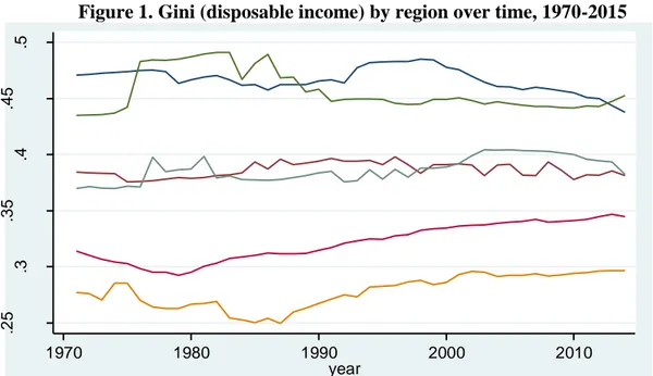
Due to high levels of income inequality around the world, many governments have made redistribution of income a major policy goal.2_{In Figure 1 we plot the median Gini coefficient on} disposable income from the Standardized World Income Inequality Database (SWIID) between 1970 and 2015 in selected geographical regions. We can observe that, at the end of the time span, sub-Saharan Africa is the region with the highest inequality.3_{While countries in Asia and the} Middle East have been relatively stable over time, there has been a rising trend in inequality in both European and North American regions.

Figure 1. Gini (disposable income) by region over time, 1970-2015

Note: blue line refers to Latin America; green line refers to Sub Saharan Africa; dark red line refers to Middle East and North Africa; grey line refers to Asia; light red line refers to North America; orange line refers to Europe. Source: SWIID

The list of underlying cyclical and structural forces affecting the level and dynamic evolution of inequality is long. These range from demographic trends to persistent cross-country differences in macroeconomic policies or different institutional settings (see e.g. Jalles and Mello, 2019). One that has been receiving growing attention is the role attributed to fiscal policy which

2_{Piketty (2014) presents a new approach to understanding the evolution of income and wealth distribution by}

examining historical evidence. According to Krugman (2014), unequal compensation and high incomes of a few individuals have led to accumulation of wealth.

3_{Gini indices are measured on a [0-100] scale with larger values denoting higher inequality.}

.2 5 .3 .3 5 .4 .4 5 .5 1970 1980 1990 2000 2010 year median_lac median_menap median_ssa median_eur median_asia median_namrc

(6)

4

shapes a country´s distribution of income and poverty (Clements et. al 2015; DeFina and Thanawala, 2004). This has made the role of government in income redistribution - in particular, the tax-benefit system – all the more relevant (Ortiz and Cummins, 2011; Rosen and Gayer, 2014).4 Governments need to strike a balance between efficiency and redistribution when designing a tax system (Clements et. al, 2015; Diamond and Mirrlees, 1971).5

Studies have shown that in many countries a substantial proportion of the poor are made poorer (or non-poor made poor) by the tax and transfer system. Higgins and Lustig (2016) find that in ten of twenty-five countries they studied at least one-quarter of the poor paid more in taxes than they received in transfers. This is because tax and transfer systems in low and middle-income countries are typically far less effective than those in OECD countries at reducing poverty and inequality (Bastagli et al., 2015). In the OECD countries, the tax and transfer systems have lowered average market income Gini by one-third (Coady et al., 2015). The relative ineffectiveness of tax and transfer systems in emerging and low-income countries is attributable to low level of revenues and poor targeting of spending programs.

As we discuss in more detail in section 2, many authors have looked at the role attributed to different taxes in affecting both economic growth and income inequality in an effort to understand taxes that make the overall revenue system pro-poor and more inclusive. The majority of these studies focus on advanced economies and many have not reached a consensus on the nature of the tax-inequality relationship (Atkinson and Leigh, 2013). Tax and revenue administration reforms are typically not randomly assigned in time and space and vary widely across developing countries, and their effects in improving income distribution, if any, are not clearly established. This paper contributes to filling this gap by analyzing the relationship between inequality and tax policy by using a new dataset that does not suffer from the limitations of cross-sectional or time units, as has been the case with other studies (e.g. Piketty and Saez, 2003). From a policy point of view, as Bird (2005) suggested, the issues related to income distribution not only are relevant to tax policy, but they also affect the minds of policy makers with regard to vertical and horizontal justice. A good understanding of the distributive impact of ordinary taxes should help in moving towards justice-oriented tax systems without sacrificing efficiency (Askari, 2011).

4_{Taxation provides resources to the government to perform critical roles such as economic stabilization, allocation}

and redistribution (Musgrave, 1959).

5_{The theory of optimal taxation looks at the tax design that seeks to maximize social welfare, an analysis that is}

(7)

5

We use a “narrative” database of major increases in government tax revenue, stemming from both improvements in revenue administration and specific tax policy measures, put together by Akitoby et al. (2019) for 45 developing economies (23 emerging and 22 low-income) during 2000 to 2015. Using this database, we estimate the dynamic short to medium-term response of income distribution proxies to different tax policy measures. An important novelty and strength of this database is the precise timing and nature of key legislative tax actions (or tax reform “shocks”) over the 15-year period. We rely on the local projection method (Jordà, 2005), which has been used to study the dynamic impact of macroeconomic shocks such as financial crises (Romer and Romer, 2017) or fiscal shocks (Jordà and Taylor, 2016). Because the short-term effects of tax reforms may differ depending on the phase of the business cycle prevailing at the time of the reform and initial conditions (such as the size of the existing tax system or general government), we also explore the role of these non-linearities in shaping the dynamic response of income distribution proxies to tax reforms6_{, using the smooth transition autoregressive model developed} by Granger and Teräsvirta (1993).

While we argue that the dataset used in the paper provides an exogenous source for tax reforms, endogeneity can still be a potentially significant concern in our framework since i) revenue mobilization efforts may not necessarily be exogenous events; and ii) several authors have found it difficult to control for the two-way causality between income and inequality in most cross-country studies. We try to address these major methodological challenges by controlling for expected economic growth at the time of revenue reforms and other possible short-term drivers of income inequality. In order to mitigate potential endogeneity concerns, we also estimate our specifications using an Instrumental Variable (IV) approach. On the one hand, to instrument revenue mobilization reforms we draw instruments from the political economy literature for the drivers of structural reforms more broadly (and not necessarily only fiscal or economic reforms in general). On the other hand, we use the growth rate of real GDP of main trading partners to instrument output growth, following Cevik and Correa-Caro (2020).

The main findings can be summarized as follows. After a general tax reform, the Gini index slowly falls, and the bottom income share slowly rises. This result is driven largely by countries

6_{See Cacciatore et al. (2016) and Duval and Furceri (2018) for examples on the nonlinear effects of reforms on}

macroeconomic variables depending on the phase of the business cycle. See IMF (2019) for the role of the fiscal stance in affecting reforms covering macroeconomic variables in developing countries.

(8)

6

outside sub-Sahara Africa. Particularly effective in improving the income distribution seems to be personal income tax (PIT) reforms and also reforms in the operation of the tax revenue administration. The results further show that the design of tax reforms has been ineffective in reducing disposable income inequality in sub-Saharan Africa; unlike other country groups, PIT reforms worsened the Gini coefficient. Our results are robust to a battery of tests including the exclusion of country fixed effects, the addition of time effects and time trends, controlling for other short-term drivers of inequality (including expectations about future growth). Conducting endogeneity robust estimations, we found stronger negative (positive) effects of tax reforms on inequality (bottom income share). We also found that in order to reduce more rapidly income inequality and improve the income prospects of the poorest strata of the population, it is more effective to implement tax reforms when the economy is growing relatively slowly. Finally, the smaller the government and the smaller the tax system, the larger the beneficial impact of tax reforms on income distribution.

The remainder of the paper is structured as follows. As background, context and motivation for our empirical analysis, Section 2 provides an overview of related literature. Section 3 presents the empirical strategy followed to study the dynamic response of income distribution proxies to revenue mobilization reforms. Section 4 presents the data and key stylized facts. Section 5 discusses the baseline empirical results, sensitivity and robustness checks. Section 6 concludes and elaborates on the policy implications.

2. Literature Review

An extensive literature is available on the determinants of income distribution.7

First and foremost, most authors tend to agree that a high degree of income inequality affects economic growth negatively (Alesina and Rodrik, 1994; Perotti, 1996; Cingano, 2014; Bourguignon, 2004; Kayizzi-Mugerwa, 2001).8_{There are several reasons for this. High inequality} is typically associated with unequal access to basic facilities and opportunities, political instability

7_{The inequality literature can be divided into two strands: the first group studies income inequality (Golding and}

Margo, 1992; Feenberg and Poterba, 1993, 2000; Frank, 2009; Atkinson et al., 2011); the other focuses on wealth inequality (Saez and Zucman, 2016; Johannesen and Zucman, 2014; Alstadsaeter et al., 2019).

8_{According to Kaldor (1995), income inequality can also be good for growth by enabling more savings and, hence,}

(9)

7

and social problems (such as crime and other conflicts and the use of illegal drugs which further worsens social inequalities) (Wilkinson and Pickett, 2010; Ortiz and Cummins, 2011). Globalization, technological change, changes in demography, unemployment and disparities in the distribution of wages and salaries are seen as the major causes of income inequality (Krugman, 2007; Kayizzi-Mugerwa, 2001; Stiglitz, 2012).

At the same time, higher taxes can generate negative consequences for growth by affecting consumption and investment decisions (Feldstein, 2012). Earlier theoretical studies on taxation show how higher taxes tend to discourage investment rates (Auerbach and Hasset, 1991) as well as labor supply of individuals (Hausman, 1985) and productivity growth, the latter adversely affecting research and development.9_{Subsequently, some authors used endogenous growth} models to simulate the effects of tax reforms on economic growth and found that a decrease in the distorting effects of the current tax structure may lead to a permanent increase in economic growth (Gale, 1996).

Much of the empirical work examining the effect of income inequality on growth argues that inequality affects growth through its effect on taxes and redistribution (Barro, 2000; Milanovic, 2002; Perotti, 1992; Persson and Tabellini, 1994). The conventional wisdom is that taxes (particularly individual and corporate) were largely motivated politically by “concerns about equity” and can help in reducing inequality and redistributing income (Burman, 2015). The general argument, based on the median voter hypothesis, is that as the ratio of median income to mean income falls the median voter will vote for higher taxes and greater redistribution.10_Therefore, greater income inequality should lead to greater progressivity.11_{Ultimately, the design of the tax} system determines its redistribution ability (Diamond and Mirrlees, 1971; Atkinson and Stiglitz, 1976; Saez, 2012).

The distribution efficiency of different taxes across countries and has been studied by e.g. Chu et al. (2000), Martinez-Vasquez et al., 2012) and Clements et. al. (2015). Some studies show that the effect of taxes on inequality and poverty is small and/or weak, more so in developing countries

9_{The main channel is that corporate and personal income taxes reduce incentives to raise supply through capital}

accumulation or productivity enhancements (Schwellnus and Arnold, 2008; Vartia, 2008; Galindo and Pombo, 2011).

10_{A small but growing number of empirical studies have examined the effect of democracy on total tax revenues and}

the composition of taxation (Aidt and Jensen, 2009; Boix, 2001; Kenny and Winner, 2006; Profeta et al., 2013).

11_{Progressive taxation was thought to be strategically important to favor a more inclusive process of economic}

development (Kaldor, 1963). How changes in tax progressivity affect income distribution has been the object of several papers at the cross-country level including Feenberg and Poterba (1993), Feldstein (1995, 1999), Piketty et al. (2014), Frey and Schaltegger (2016) and Saez (2017).

(10)

8

(e.g. Bird and Zolt, 2014). The reason as noted earlier is that in developing countries, tax-benefit systems are less developed and, therefore, potentially less redistributive, there is greater reliance on indirect taxes (compared with advanced economies), lower progressivity in direct tax schedules and less comprehensive formal social safety nets.12_{According to Prasad (2008), there are four main} reasons why developing countries rely more heavily on indirect taxes than direct taxes. First, given their low-income level, the tax base is relatively small and, as a result, indirect taxes represent an easier way to collect government revenue (Bahl and Bird, 2008; Casale, 2012). Second, the efficiency of collecting direct taxes in developing countries is often poor. Third, income tax evasion is high. Fourth, developing countries have a large informal sector which does not pay income taxes.

There are several reasons why developing countries are less capable of using the tax system to redistribute (Bastagli et al., 2015). First, income and wealth taxes play a relatively small role in their tax structure compared with advanced economies. Second, the personal income tax in developing countries is often a merely wage withholding tax.13_{The limited ability of the personal} income tax to tax effectively income from most forms of capital may suggest that it is less likely that the rich would bear significant tax liability. Third, it may be politically difficult to impose effective income tax and wealth taxes in many countries.

Despite the prevalence of redistribution as a guiding motive in the design of tax systems in developed countries, poverty and/or inequality considerations have generally been of secondary importance in developing countries´ fiscal reforms. A growing body of literature has documented the positive effect of the tax reforms of the 2000´s in reducing income inequality in Latin America (Jimenez et al., 2010; Cetrangoilo and Gomez Sabaini, 2007; Hanni et al., 2015).14_{Ideally, this} should be achieved while minimizing distortionary effects on growth caused by taxation.15

12_{In the case of Latin America, for example, incidence analysis shows that the redistributive impact of tax-benefit}

systems varies considerably from country to country, and it tends to be stronger in Argentina, Brazil and Uruguay (Brezzi and de Mello, 2016), although they are considerably less redistributive than in advanced economies. Ilaboya and Ohonba (2013) found that tax burden has a significant negative effect on income inequality in Nigeria (using household survey data).

13_{In many countries taxes on labor in the formal sector comprise over 90 percent of the total individual income tax}

revenue. In some countries, the tax law does not reach income from capital, such as capital gains. In other countries, the limitations of tax administrations may effectively exempt certain types of income from tax.

14_{This contrasts with earlier findings that taxation had a negligible effect on income inequality in Latin American}

countries in previous decades (Cornia et al., 2011).

15_{Empirically, a number of studies support the hypothesis that distortive taxes hold back growth more than others}

(Kneller et al., 1999; Gemmel et al., 2011, 2014; Johansson, 2016; Drucker et al., 2017). Corporate and personal income taxes are considered more distortionary than consumption or property taxes as shown by Arnold et al. (2011).

(11)

9

Common reforms include a shift from trade taxes to domestic sales taxes, the rationalization of income taxes and increase of its progressivity16_{, and measures to reduce budget deficits and/or} raise tax-to-GDP ratios while improving the efficiency of tax collection (IMF, 2014). Another commonly considered policy action includes the shift of the revenue mix away from corporate or personal income tax towards consumption (value-added) and property taxes, which could be growth-enhancing. Indeed, Acosta-Ormaechea and Yoo (2019) confirmed that consumption and property taxes are more growth friendly than income taxes. Similarly, McNabb and LeMay-Boucher (2014) and Drucker et al. (2017) found that reducing the share of income taxes in the revenue mix would raise GDP growth.

Most cross-country empirical studies support that direct taxes are progressive hence they are better instruments to redistribute income than indirect taxes (Obadic et al., 2014; Saez, 2010; Barnard, 2010; Weller, 2008).17_{Consumption taxes negatively affect income distribution} (Martinez-Vasquez et al., 2012; Karanfil and Ozkaya, 2013). The efficiency of consumption taxes and its role in enhancing equity was examined in a qualitative study by Correia (2007). For efficiency purposes a single rate is preferred to increase the revenue yield, combined with a well targeted transfer program (Engel et al. 1999; Okner, 1975). The more the consumption taxes contribute to the government revenue, the stronger are the effects on efficiency and welfare for the low-income earners. This view of consumption tax contrasts with the common view that these taxes are regressive.18_{This regressivity can be mitigated by having differentiated rate; lower rates} for basic goods and higher rate for luxury goods, though this complicates the tax administration and is sub-optimal (Saez, 2010). Higher VAT thresholds for registration of traders can also obviate the regressivity associated with consumption tax since the poor tend to buy more from small traders. AfDB (2010) advocates removal of tax exemptions and incentives in the Kenya tax system as they undermine tax equity and lead to revenue losses. Askari (2011), analyzing the Iranian case, finds that direct taxes affect income distribution negatively due to tax evasion while indirect taxes

16_{In the post-WWII period policymakers assigned to taxation the specific role of promoting redistribution through the}

introduction of high taxes on income (Cornia et al., 2011). Recent public debate has focused on the role of income taxes in reducing inequality (Atkinson, 2015; Piketty, 2014).

17_{The main reason is that, while consumption and property taxes are close to proportional - all individuals are subject}

to the same tax rate irrespective of their level of income -, personal income taxes are typically progressive. In developing countries in particular consumption taxes are borne by all consumers both in the formal and informal sector, while personal and corporate income taxes are usually paid by firms in the formal sector; the informal sector escapes paying income taxes.

18_{Swistak et al. (2015) analyzing value-added tax reforms in Poland found these to be regressive. According to Saez}

(12)

10

have a positive impact on income distribution. Karanfil and Ozkaya (2013) find that indirect taxes have a long run positive impact on poverty in Turkey. Saez (2016) finds that the 2013 US tax increase of the top marginal rate had a large negative effect on reported income at the top.

This paper contributes to the literature on income inequality drivers by looking specifically at the role played by tax reforms by category, which has been largely overlooked and for which there is no consensus.

3. Econometric Methodology

In order to estimate the dynamic response of income distribution proxies to tax revenue reforms, we follow the local projection method proposed by Jordà (2005) to estimate impulse-response functions. This approach has been advocated by Auerbach and Gorodnichenko (2013) and Romer and Romer (2017) as a flexible alternative to vector autoregression (autoregressive distributed lag) specifications since it does not impose dynamic restrictions. It is better suited to estimating nonlinearities in the dynamic response—such as, in our context, interactions between tax reform shocks and macroeconomic conditions. The baseline specification is:

𝑦𝑡+𝑘,𝑖 − 𝑦𝑡−1,𝑖 = 𝛼𝑖 + β𝑘𝑅𝑖,𝑡+ 𝜃𝑋𝑖,𝑡+ ε𝑖,𝑡 (1) in which y is the dependent variable of interest, namely an income distribution proxy19_{; 𝛽}

𝑘 denotes the (cumulative) response of the variable of interest in each k year after the tax revenue reform; 𝛼_𝑖 are country fixed effects, included to take account of differences in countries’ average current account balance; 𝑅_𝑖,𝑡 denotes the tax revenue reform shock in the area considered - if there are sequences of years with the same type of reform, we focus only on the first year of a given tax reform episode to improve the identification and minimize reverse causality problems (for a similar approach see Ball, Furceri, Leigh, Loungani, 2013).20_𝑋

𝑖,𝑡 is a set a of control variables including two lags of tax reform shocks, two lags of real GDP growth and two lags of the dependent variable. Equation (1) is estimated using OLS. Impulse response functions (IRFs) are then obtained by plotting the estimated 𝛽𝑘 for k= 0,1,..5 with 90 (68) percent confidence bands computed using the

19_{Since both poverty and income inequality are both aspects of income distribution, we employ as dependent variables}

both Gini measures and also income shares of the top and bottom deciles of the population.

(13)

11

standard deviations associated with the estimated coefficients 𝛽𝑘—based on robust standard errors clustered at the country level.21_{According to Sims and Zha (1999) “the conventional pointwise} bands common in the literature should be supplemented with measures of shape uncertainty”. Hence, for characterizing likelihood shape, bands that correspond to 68 percent posterior probability - or one standard deviation shock - provide a more precise estimate of the true coverage probability.22_{An important issue raised by some scholars (Piketty and Saez, 2007; Poterba, 2007)} is the potential reverse causation between economic inequality and taxation that may generate an endogeneity problem in the relationship under consideration. According to this rationale, lower degrees of economic inequality may be the contemporaneous result of a more redistributive tax structure (i.e. a tax structure imposing a large tax burden on capital relative to labor) rather than solely the cause of it. Tax revenue reforms may not be entirely exogenous shocks as they could be potentially anticipated, correlated with past changes in economic activity and implemented because of concerns about fiscal sustainability or other important developmental needs. The same is true with respect to the potential endogeneity of income in affecting inequality dynamics. These potential methodological limitations are dealt with by relying on tax data constructed to reflect the relevant tax legislation and, therefore, are exogenous to the general economic conditions and to any indirect channel that may affect the realized tax policy. Technically these limitations are addressed in Section 5 with a series of robustness checks, including the use of an Instrumental Variable (IV) approach. For tax reforms, we rely on instruments from the political economy drivers of reforms. Regarding the potential non-exogeneity of income, we follow Cevik and Correa-Caro (2020) that instrument it using the growth rate of main trading partners.

4. Data and Stylized Facts

4.1 Income Distribution

Income inequality proxies, namely the Gini index, is obtained from the Standardized World Income Inequality Database (SWIID), constructed by Solt (2009) using the UN World Income Database and the Luxembourg Income Study. Taxes determine the disposable income available

21_{Another advantage of the local projection method compared to vector autoregression (autoregressive distributed}

lag) specifications is that the computation of confidence bands does not require Monte Carlo simulations or asymptotic approximations. One limitation, however, is that confidence bands at longer horizons tend to be wider than those estimated in vector autoregression specifications.

22_{Other papers that have employed one standard deviation bands include e.g. Giordano et al. (2007), Romer and}

(14)

12

for consumption to the households and thus influence income distribution. However, the disposable income does not take into account indirect taxes (Karanfil and Ozkaya, 2013). This creates a limitation when only disposable income is considered. As a result, we look at both pre-tax-and-transfers and post-pre-tax-and-transfers Gini indices.23_{According to Poterba (2007), this also} mitigates the reverse causality problem since post-tax-and-transfers vary “mechanically” and “economically” with the fiscal system whereas the pre-tax-and-transfers measure vary solely through the endogenous responses of labor supply or the general equilibrium effect on factor prices. In fact, the SWIID provides comparable estimates for two definitions of the Gini coefficient - the first based on market income and the second net of taxes and transfers – on an annual basis. This allows us to assess income inequality before and after fiscal redistribution through tax reforms and provides comparable Gini figures across countries and over a long span of time. However, the imputation methodology to standardize observations collected from various sources makes these series subject to measurement uncertainty (Jenkins, 2015).24_{Ferreira et al. (2015) compared eight} inequality datasets25_{to conclude that “although there is much agreement across these databases,} there is also a non-trivial share of country/year cells for which substantial discrepancies exist” and that “the methodological differences […] often appear to be driven by a fundamental trade-off between a wish for broader coverage on the one hand, and for greater comparability on the other”.26

As a complement, we use the top and bottom 10 percent income shares retrieved from the World Bank´s World Development Indicators (WDI).

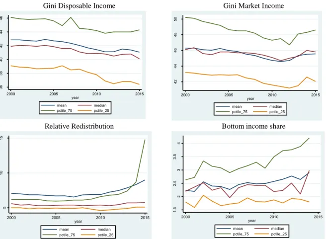
Guided by the tax reform data we focus on a panel of 45 developing countries between 2000-2015.27_{Based on this sample, Figure 2 shows the interquartile range of alternative proxies} for income distribution. We observe that over the last 15 years inequality, as measured by

23_{The Gini indicators based on disposable income cover the total market income received by all household members}

(gross earnings, self-employment income, capital income), plus the current cash transfers they receive, less income and wealth taxes, social security contributions and current transfers that they pay to other households.

24_{Multiple imputation methods are used which essentially rely on assuming that ratios between different inequality}

measures are constant, or stable, and can therefore be used to predict those variables when they are not observed (Solt, 2009).

25_{Five are microdata-based: CEPALSTAT, Income Distribution Database (IDD), LIS, PovcalNet, and}

Socio-Economic Database for Latin America and the Caribbean (SEDLAC); two are based on secondary sources: “All the Ginis” (ATG) and the World Income Inequality Database (WIID); and one is generated entirely through multiple-imputation methods: the Standardized World Income Inequality Database (SWIID).

26_{As this paper places a special emphasis on the Sub-Saharan African (SSA) region, we decided to maximize coverage.}

For instance, the WIID includes 350 inequality observations for SSA between 1960-2012 of which only five are labeled high quality, while the SWIID – which we use – includes 934 observations for this region and treats all of them as comparable in quality terms.

(15)

13

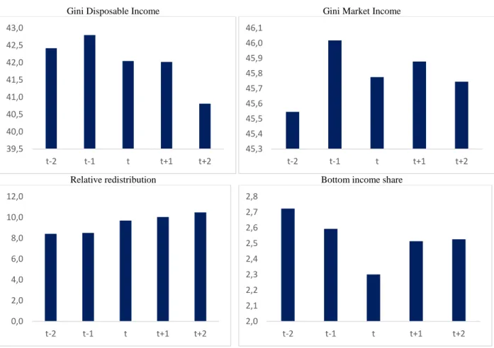
disposable income has been on a downward trend but this fact is often obscured by the fact that market Gini has been increasing since the early 2010´s. This points to a useful and powerful role of the tax-benefit redistributive systems in these countries in recent years (see bottom left panel).28 As inequality and poverty while different are related concepts and then to go hand-in--hand, in the bottom right panel, we can see that the income share of the bottom 10 percent of the population has also been on the rise.

Figure 2. Interquartile Range of Income Distribution Proxies over time, 2000-2015

Gini Disposable Income Gini Market Income

Relative Redistribution Bottom income share

Note: figure plots the average (mean), median, bottom and top quartiles (pctile_25 and pctile_75, respectively) of respective variables´ distributions. Relative redistribution measures the difference between market and disposable Gini indices. The bottom income share corresponds to the income share of the bottom 10 percent of the population. Source: SWIID and WDI.

There is significant dispersion across economies in terms of income inequality. It is essential to analyze the time series properties of the data to avoid spurious results by conducting

28_{Redistribution is typically defined as the difference between market income and disposable income inequality. Some}

authors then express it as a percentage of market income inequality.

36 38 40 42 44 46 2000 2005 2010 2015 year mean median pctile_75 pctile_25 42 44 46 48 50 2000 2005 2010 2015 year mean median pctile_75 pctile_25 5 10 15 2000 2005 2010 2015 year mean median pctile_75 pctile_25 1 .5 2 2 .5 3 3 .5 4 2000 2005 2010 2015 year mean median pctile_75 pctile_25

(16)

14

panel unit root tests. We check the stationarity of all variables by applying the Im-Pesaran-Shin (2003) procedure, which is widely used in the empirical literature dealing with non-stationary panels. The results, available upon request, indicate that the Gini indices used in the analysis are stationary after logarithmic transformation.

4.2 Tax Reforms

Countries determine the composition of their tax system by making policy changes to tax bases, tax rates and exemptions. The tax reform database put together by Akitoby et al. (2019) is now explored carefully in this paper. In identifying the episodes of large tax revenue mobilization, Akitoby et al. (2019) focused on countries with more tangible tax revenue mobilization results; (i) countries that have increased their tax-to-GDP ratios by a minimum of 0.5 percent each year for at least three consecutive years (or 1.5 percent within three years); (ii) countries with beyond average increases in their tax-to-GDP ratios; and/or (iii) countries with better tax performance compared with peers in the same income group (see original source for further details).

This tax reform database has several advantages for our own empirical purposes: it identifies the precise nature and exact timing of major tax actions in key areas of tax policy and revenue administration; identifies the precise tax reforms that underpin what otherwise looks like a gradual improvement in standard tax-to-GDP; identifies major reforms that truly led to increases in revenue, as opposed to just a long list of (small or not economically meaningful) policy changes. All these aspects of data are particularly useful for empirical analysis that seeks to identify, and then estimate, the dynamic effects of tax reform shocks. The strengths of this “narrative” tax reform database come with one limitation; because two large reforms in a given area (for example, a change in Personal Income Tax) can involve different specific actions (for example, tax introductions (“new taxes”), rate changes, threshold changes and changes to exemptions), only the average impact across major historical tax reforms can be estimated. It should be noted that the tax reform database provides no information regarding the current (or past) fiscal stance in the countries under scrutiny, which is not the purpose of this paper.

Tables 1-3 present stylized facts on reforms in the following categories: personal income tax (PIT), corporate income tax (CIT), goods and services taxes split between 3 subcategories (value added taxes (VAT), excises and general other goods and services taxes), trade taxes,

(17)

15

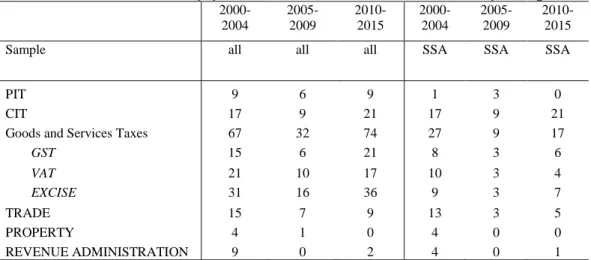
property taxes and, finally, revenue administration.29_{The vast majority of tax revenue reforms in} our sample were in the category of goods and services taxes and most reforms were implemented during the period 2010-2015 (Table 1). Exceptions are, e.g., tax reforms in the area of excises, trade or property, which were implemented more during 2000-2004. In SSA the majority of tax revenue reforms were in the area of goods and services, and during the 2000-2004 period. In the more recent period, SSA has been focusing more on CIT reforms.

Table 1. Number of country-years with tax mobilization shocks by sub-periods

2000-2004 2005-2009 2010-2015 2000-2004 2005-2009 2010-2015

Sample all all all SSA SSA SSA

PIT 9 6 9 1 3 0

CIT 17 9 21 17 9 21

Goods and Services Taxes 67 32 74 27 9 17

GST 15 6 21 8 3 6 VAT 21 10 17 10 3 4 EXCISE 31 16 36 9 3 7 TRADE 15 7 9 13 3 5 PROPERTY 4 1 0 4 0 0 REVENUE ADMINISTRATION 9 0 2 4 0 1

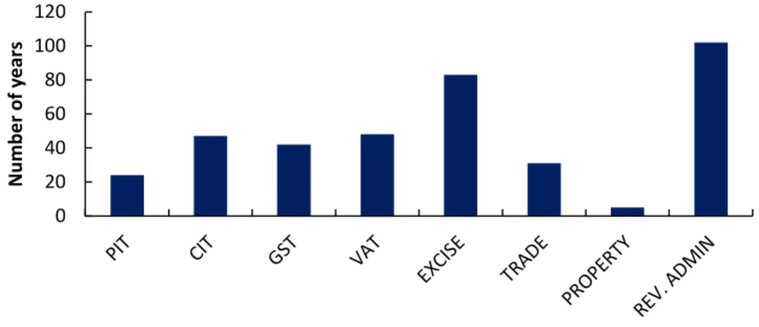
Figure 3 provides the number of years of tax reforms identified in the sample and illustrates the heterogeneity of reforms efforts by type. Excise reforms have been more frequently implemented. In general, fewer major reforms have been implemented in the areas of property taxes. Reforms in tax administration have been more the rule than the exception, acompanying a specific tax policy measure. Out of 119 years of tax reforms, only 17 correspondend to tax policy measures not acompanied by improvements in revenue administration.

29_{Revenue administration reforms includes measures in 8 distinct areas, namely: i) management, governance and HR;}

ii) large taxpayers office and segmentation; iii) IT system; iv) registration and filling; v) audit and verification; vi) management of payment obligations; vii) improving compliance; viii) customs clearance. According to Akitoby et al. (2019), hiring more qualified staff, strategic planning and monitoring performance, focusing on training and strengthening tax legislation to empower revenue collection agencies were the most commonly implemented measures (77 percent of episodes).

(18)

16

Figure 3. Number of country-years with tax revenue reforms by type (45 developing economies, 2000-2015)

In terms of geographical distribution, emerging market economies did more reforms in the area of personal income tax, value-added and excises, while low-income countries focused more on trade taxes (Table 2). As for other categories of taxes both groups are comparable and also when it comes to revenue administration reforms.

Table 2. Reform shocks by group of countries (number of tax reform country-years)

EME LIC SSA Resource-

Rich

Fragile

Number of countries 23 22 10 6 13

PIT 16 8 4 2 4

CIT 23 24 12 4 6

Goods and Services Taxes 99 74 53 14 49

GST 20 22 17 2 10 VAT 30 18 17 0 17 EXCISE 49 34 19 12 22 TRADE 10 21 21 5 15 PROPERTY 1 4 4 0 4 REVENUE ADMINISTRATION 57 45 33 7 24

Finally, tax reforms have been more frequently implemented during periods of higher economic growth—that is when the real GDP growth in each country was above its historical average(Table 3). 0 20 40 60 80 100 120 N u m b e r o f y e ar s

(19)

17

Table 3. Tax Reform shocks over the business cycle (number of tax reform country-years)

Lower economic growth Higher economic growth PIT 8 16 CIT 20 27

Goods and Services Taxes 75 98

GST 17 25 VAT 20 28 EXCISE 38 45 TRADE 10 21 PROPERTY 2 3 REVENUE ADMINISTRATION 48 54

Note: lower (higher) economic growth = real GDP growth below (above) the reforming country’s historical average.

Descriptive statistics on different income distribution proxies before and after the beginning of these tax revenue reform episodes suggest that tax reforms have on average been associated with a decrease in the Gini index based on disposable income in the years after the reform (Figure 4). The fall in the Gini index based on disposable income is larger than the one based on market income, meaning an improvement in redistribution in the years after a tax reform, reflecting both the impact of taxes and increased capacity of governments to fund transfer programs. This is consistent with an increase in the income share of the bottom 10 percent of the population. Section 4 tests whether this (unconditional) suggestive evidence holds up to more formal tests.

(20)

18

Figure 4. Evolution of income distribution proxies around Tax Revenue Reforms

Gini Disposable Income Gini Market Income

Relative redistribution Bottom income share

Note: x-axis in years; t=0 is the year of the tax reform shock.

4.3 Other Data

Real GDP comes from the IMF´s World Economic Outlook (WEO) database and tax variables from the World Bank´s World Development Indicators (WDI). Specifically, by analyzing different tax categories in percent of GDP for the sample of 45 countries in our panel we get the interquartile range dynamics depicted in Figure 5.

39,5 40,0 40,5 41,0 41,5 42,0 42,5 43,0 t-2 t-1 t t+1 t+2 45,3 45,4 45,5 45,6 45,7 45,8 45,9 46,0 46,1 t-2 t-1 t t+1 t+2 0,0 2,0 4,0 6,0 8,0 10,0 12,0 t-2 t-1 t t+1 t+2 2,0 2,1 2,2 2,3 2,4 2,5 2,6 2,7 2,8 t-2 t-1 t t+1 t+2

(21)

19

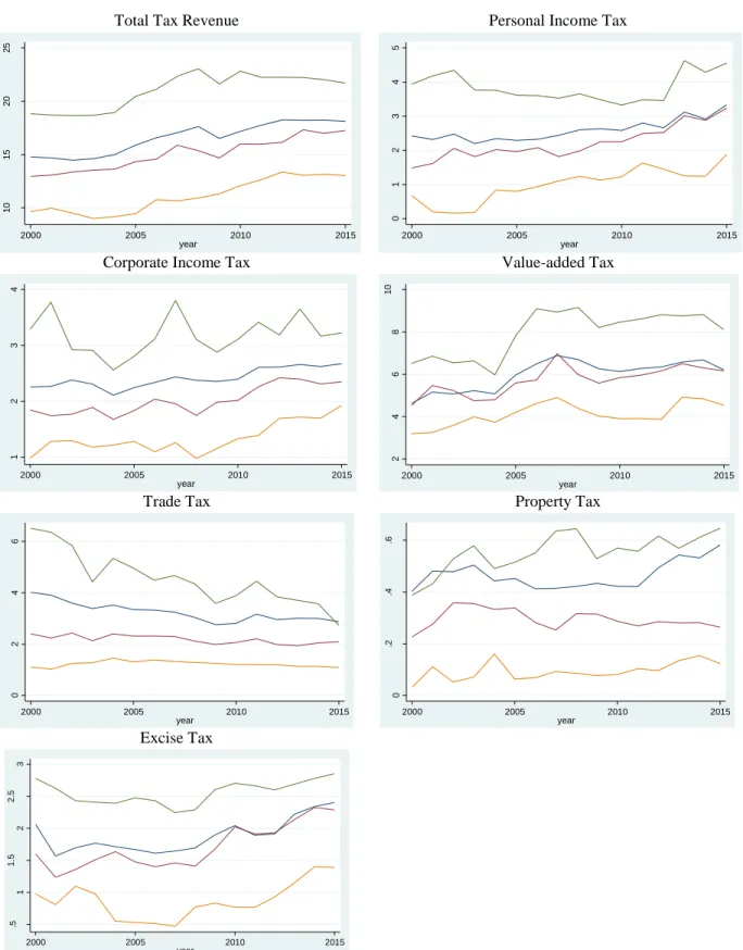
Figure 5. Composition of tax revenues (% GDP) in 45 developing countries, 2000-2015

Total Tax Revenue Personal Income Tax

Corporate Income Tax Value-added Tax

Trade Tax Property Tax

Excise Tax

Note: green line denotes the 75th_{percentile of the respective distribution; the blue line denotes the mean; the red line}

denotes the median; and the yellow line denotes the 25th_{percentile of the respective distribution. All charts expressed}

in percentage of GDP. Source: IMF WEO.

10 15 20 25 2000 2005 2010 2015 year mean median pctile_75 pctile_25 0 1 2 3 4 5 2000 2005 2010 2015 year mean median pctile_75 pctile_25 1 2 3 4 2000 2005 2010 2015 year mean median pctile_75 pctile_25 2 4 6 8 10 2000 2005 2010 2015 year mean median pctile_75 pctile_25 0 2 4 6 2000 2005 2010 2015 year mean median pctile_75 pctile_25 0 .2 .4 .6 2000 2005 2010 2015 year mean median pctile_75 pctile_25 .5 1 1 .5 2 2 .5 3 2000 2005 2010 2015 year mean median pctile_75 pctile_25

(22)

20

Note that according to the summary statistics present in Table A1 in the appendix, we will focus, in what follows, on those reforms with the largest distributional impact based on their importance measured in terms of corresponding tax shares to GDP. Taxes on goods and services, in the last year considered 2015, averaged 6 percent of GDP in the sample of countries considered. This was followed by PIT and then Trade and CIT. Lastly, property taxes accounted for a relatively small amount in GDP terms (only 0.6 percent).

5. Empirical Results

A. Baseline

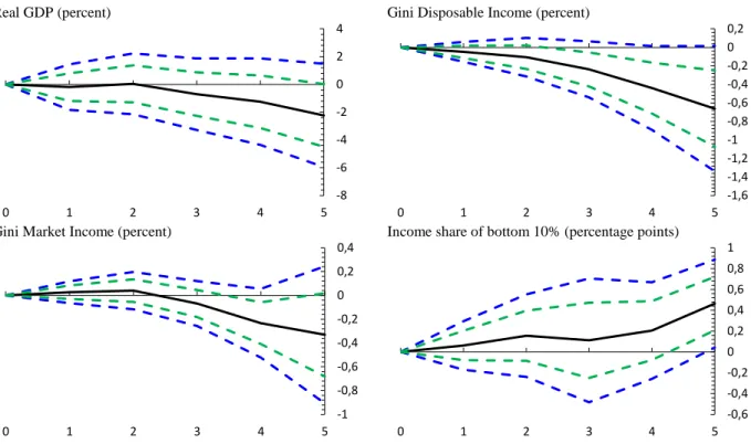
Figure 6 shows the results of estimating equation (1) for alternative dependent variables. Both the 90 and 68 percent confidence bands are shown. After a general tax revenue mobilization reform takes place real GDP growth does not seem to be initially affected, starting a decline after 2 years but the effect is not statistically different from zero even after 5 years. In contrast, it seems that inequality goes down and the effect is particularly visible when using the Gini index based on disposable income. After 5 years the Gini falls by 0.7 percent (which corresponds to one standard deviation – the situation that took place in Uruguay in 2002 or Guinea-Bissau in 2004) and this effect is statistically significant at the 90 percent confidence level. The effect is not as strong in magnitude and significance when employing the Gini index based on market income, but still the downward sloping reaction stands out. Complementary, a general tax reform can help improving the income share of the bottom 10 percent of the population by 0.5 percentage points (or two standard deviations – the situation that took place in Kyrgyzstan in 2010) after 5 years. These effects show that there is merit in using the tax system for redistribution purposes. Note however that redistribution reflects not only the impact of taxes on economic agents who have the ability to pay them but also the effect of transfer programs.

(23)

21

Figure 6. Impact of Tax Revenue Reforms on Different Variables

Real GDP (percent) Gini Disposable Income (percent)

Gini Market Income (percent) Income share of bottom 10% (percentage points)

Note: x-axis in years; t=0 is the year of the tax reform shock. Solid black lines denote the response to a tax reform shock, blue dashed lines denote 90 percent confidence bands and green dashed lines denote 68 percent confidence bands, based on standard errors clustered at country level.

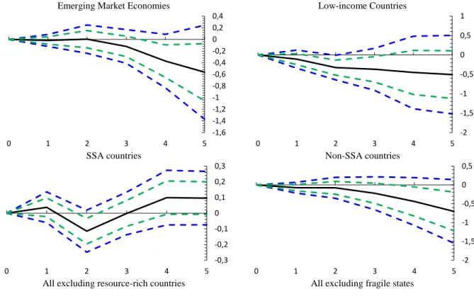
Splitting the sample of 45 countries by income group and geographical region and performing sensitivity with respect to country characteristics (such as being a fragile state30_{or a} resource-rich economy31_{) yields the results in Figure 7 for the Gini index based on disposable} income. We observe that the negative impact of tax reforms on inequality is strongest in emerging market economies possibly due to the fact that these countries´ tax system is more mature and well-established. In the middle panel, we observe that the overall sample result is being driven by countries outside of-sub-Saharan region as the effect of tax reforms in sub-Saharan African is not statistically different from zero. This potentially highlights the lack of income distribution considerations embedded in tax reforms implemented in Africa (who happen to be largely fragile states) and/or the lack of transfer programs in these countries and/or inability of tax reforms to

30_{In one of the sensitivity analyses conducted, tax reform episodes in fragile states are excluded given their rather}

unique social and economic characteristics. More recent research has shown (Baer and others, 2020) that tax reform design in fragile states should be different from that adopted in other developing countries. In our sample of 10 fragile states, 7 are in SSA.

31_{Recently, Davis (2019) tested the proposition that economies specializing in mining and oil production have high}

income inequality. He found it to be true in the case of mining but not in the case of oil production.

-8 -6 -4 -2 0 2 4 0 1 2 3 4 5 -1,6 -1,4 -1,2 -1 -0,8 -0,6 -0,4 -0,2 0 0,2 0 1 2 3 4 5 -1 -0,8 -0,6 -0,4 -0,2 0 0,2 0,4 0 1 2 3 4 5 -0,6 -0,4 -0,2 0 0,2 0,4 0,6 0,8 1 0 1 2 3 4 5

(24)

22

make a perceptible difference to tax-to-GDP ratios in these countries. Results are slightly stronger when removing either fragile states or those rich in natural resources, with a fall in the Gini index of 0.8 percent 5 years after the reform. Fragile states have extremely weak fiscal systems and resource-rich countries tend to rely less on non-resource domestic taxes. That said, all in all, outliers or specific groups of countries do not seem to be affecting greatly the result found in Figure 6.32

Figure 7. Impact of Tax Revenue Reforms on the Gini Index (Disposable Income) by Group of countries (percent)

Emerging Market Economies Low-income Countries

SSA countries Non-SSA countries

All excluding resource-rich countries All excluding fragile states

32_{We also tested whether countries – in our sample – with an IMF-supported program yielded different distributional}

effects after tax reforms compared to those not under a program. Results (not shown but available upon request) suggest that countries not under an IMF-supported program achieved larger and significant falls in disposable income Gini vis-à-vis those countries with a program (in which the dynamic effects on the Gini index are not statistically different from zero throughout the considered time horizon).

-1,6 -1,4 -1,2 -1 -0,8 -0,6 -0,4 -0,2 0 0,2 0,4 0 1 2 3 4 5 -2 -1,5 -1 -0,5 0 0,5 1 0 1 2 3 4 5 -0,3 -0,2 -0,1 0 0,1 0,2 0,3 0 1 2 3 4 5 -2 -1,5 -1 -0,5 0 0,5 0 1 2 3 4 5

(25)

23

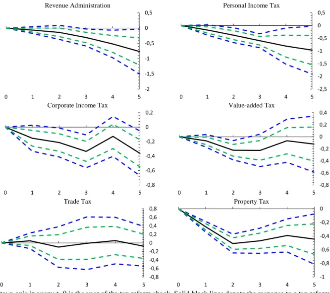
A relevant question is whether the effect of tax revenue reforms on inequality varies by tax policy instrument. To address this question, we re-estimate our main equation (1) for tax reforms in the each of the following individual tax areas: personal income tax, corporate income tax, value-added tax, trade taxes, property taxes and revenue administration reforms.33

Results suggest that reforms in all of these individual tax categories are associated with a decline in the Gini index, with the effect being larger (in absolute value) for personal income tax as one would expect, followed by revenue administration reforms which tend to improve tax compliance, property taxes and corporate income taxes (Figure 8). In particular, by conducting an independent analysis on each of the eight revenue administration categories (cf. footnote 29), results show that measures dealing with large taxpayers office and segmentation of revenue administration and customs clearance seem to be the most important in lowering the Gini index in the short run and medium-run, respectively.34

Note that our results confirm those found by Cevik and Correa-Caro (2020) for a sample of transition economies that income tax helped improve income distribution. Statistical significance of personal income tax is larger than when considering our aggregate tax reform variable (that adds up all of the reforms in all individual tax categories) because some of these individual sector reforms were implemented simultaneously. The negative impact of value-added and trade taxes is smaller and the latter also marked by a higher degree of uncertainty, as evidenced by wide confidence bands above and below zero. For SSA countries (not shown), we observe that revenue administration reforms did not have any statistically significant impact on income

33_{Other less important taxes such as excises or subsidies are omitted for reasons of parsimony but available upon}

request.

34_{Results are shown in Figure A1 in the Appendix.} -2 -1,5 -1 -0,5 0 0,5 0 1 2 3 4 5 -2 -1,5 -1 -0,5 0 0,5 0 1 2 3 4 5

(26)

24

distribution over the period under scrutiny. In contrast, it seems that in the very short-run, PIT reforms led to a worsening of the Gini index.

Figure 8. Impact of Tax Revenue Reforms on the Gini Index (Disposable Income) (percent)

Revenue Administration Personal Income Tax

B. Robustness

Sensitivity

A possible bias from estimating equation (1) using country-fixed effects is that the error term may have a non-zero expected value, due to the interaction of fixed effects and country-specific developments (Tuelings and Zubanov, 2010). This would lead to a bias of the estimates that is a

-2 -1,5 -1 -0,5 0 0,5 0 1 2 3 4 5 -2,5 -2 -1,5 -1 -0,5 0 0,5 0 1 2 3 4 5 -0,8 -0,6 -0,4 -0,2 0 0,2 0 1 2 3 4 5 -0,8 -0,6 -0,4 -0,2 0 0,2 0,4 0 1 2 3 4 5 -0,8 -0,6 -0,4 -0,2 0 0,2 0,4 0,6 0,8 0 1 2 3 4 5 -1 -0,8 -0,6 -0,4 -0,2 0 0 1 2 3 4 5

(27)

25

function of k. To address this issue, equation (1) was re-estimated by excluding country fixed effects from the analysis. Results in Figure 9 (top panel) suggest that this bias is negligible.

The baseline specification does not include year fixed effects to allow for waves of tax reforms, that is, the possibility that different types of tax policy and revenue administration reforms may occur within the same year. Indeed, in these circumstances, including time fixed effects would “partial-out” these reforms and affect the overall estimated effects of tax reforms on income distribution. To check the robustness of our results, we re-estimate equation (1) including year fixed effects. The estimated effects of tax reforms on inequality without year fixed effects are presented in Figure 9 (middle panel) and do not change the main thrust of our results.

In addition, to try and estimate the causal impact of tax reforms on income distribution proxies, it is important to control for previous trends in dynamics of the Gini index or income shares that could lead to tax reforms. The baseline specification attempts to do this by controlling for up to two lags in the dependent variable.35_{To further mitigate this concern, we re-estimate} equation (1) by including country-specific time trends as additional control variables. Results in Figure 9 (bottom panel).

Figure 9. Sensitivity: Impact of Tax Revenue Reforms

No country effects

Gini Disposable Income (percent) Income share of Bottom 10% (percentage points)

Time effects

35_{Similar results are obtained when using alternative lag parametrizations. Results for zero, one and three lags (not}

shown) confirm that previous findings are not sensitive to the choice of the number of lags.

-2 -1,5 -1 -0,5 0 0,5 0 1 2 3 4 5 -1 -0,5 0 0,5 1 1,5 0 1 2 3 4 5

(28)

26 Time trends

Controlling for additional short-term drivers of inequality

Another possible concern regarding the analysis is that the results may suffer from omitted variable bias, as reforms may be carried out because of past economic conditions or past concerns on public finances´ sustainability or at the same time as other macroeconomic policy actions that affect income distribution proxies. To address this issue, we expand the set of controls to include other variables that have been typically found to affect the evolution of inequality (see e.g. Jalles and Mello, 2019; Cevik and Correa-Caro, 2020). In particular, we include the following additional control variables: real GDP per capita; trade openness (given by the sum of exports and imports over GDP); government expenditure (% GDP); old age dependency ratio; share of value added in agriculture (% GDP). These controls are retrieved from the World Bank´s World Development Indicators. The economic rationale behind their inclusion in the augmented vector X of equation (1) is as follows. The inclusion of real GDP per capita stems from the empirical debate around the notion of the Kuznets curve – the nonlinear (U-shaped) relationship between economic development and inequality. As for the role of globalization – here proxied by trade openness – there is no consensus in the empirical literature: some argue that it benefits the poor (see e.g. Dollar and Kraay, 2004), while others show that greater openness increases inequality especially in countries with higher income levels (see e.g.

-2 -1,5 -1 -0,5 0 0,5 0 1 2 3 4 5 -0,8 -0,6 -0,4 -0,2 0 0,2 0,4 0,6 0,8 0 1 2 3 4 5 -1,5 -1 -0,5 0 0,5 0 1 2 3 4 5 -1 -0,5 0 0,5 1 0 1 2 3 4 5

(29)

27

Milanovic, 2005). There is also a literature negatively relating the size of the public sector (and its redistributive power) and income inequality. In a recent work, Guzi and Kahanec (2018) found, using a new instrumental variable approach, that much of the literature underestimates the true role of the government (measured as government expenditure over GDP) in attenuating income inequality. Deaton and Paxson (1997) found that an increase in the share of the population older than 65 tended to worsen income inequality and for this reason the age-dependency ratio is included.

Figure 10 shows the results of the augmented regression. We observe that the effect on the Gini index based on disposable income is not statistically significantly different from the baseline result in Figure 6. As for the income share of the bottom 10 percent of the population, now the impulse response is negative but statistically not different from zero in contrast with the baseline result that found some positive impact 5 years after the tax reform.

Figure 10. Additional Controls: Impact of Tax Revenue Reforms

Controlling for Growth expectations

Yet another issue is the fact that tax reforms could be implemented because of concerns regarding future evolution of economic activity. To address this issue, we control for the expected values in t-1 of future real GDP growth over periods t to t+k—that is, the time horizon over which the impulse response functions are computed. These are taken from the fall issue of the IMF World

Economic Outlook for year t-1. Figure 11 shows the results from considering growth expectations

in our baseline specification. We observe that these are in line with those presented in Figure 6. -1 -0,8 -0,6 -0,4 -0,2 0 0,2 0,4 0 1 2 3 4 5 -0,8 -0,6 -0,4 -0,2 0 0,2 0,4 0 1 2 3 4 5

(30)

28

Figure 11. The role of expectations: Impact of Tax Revenue Reforms

Dealing with endogeneity: Instrumental Variable Estimation

While the previous robustness checks go a long way toward mitigating endogeneity concerns, we still check the robustness of our results by using an Instrumental Variable (IV) approach. The literature has put forward several theories to rationalize why and when reforms (do not) happen. We focus on one broad factor examined in the literature: political institutions (see Duval, Furceri and Miethe, 2018). Specifically, we use the following set of political economy variables as external instruments which we divide in four categories: i) ideology of the governing party/ies, using a discrete variable to distinguish between left, center and right (3, 2 and 1, respectively);36_{ii) political} system, using a discrete variable for parliamentary, assembly-elected and presidential forms of governments (2, 1 and 0, respectively);37_{iii) party fragmentation, using a continuous variable} bounded between 0 (no fragmentation) and 1 (maximum fragmentation) to capture the number of political parties in the lower house of the legislative assembly;38_{iv) the strength of democratic} institutions (measured as polity IV and normalized between 0 and 1).39_{Data on these variables are} taken from the World Bank Database of Political Institutions.

36_{Right-wing governments have been associated with more market-oriented reforms (Alesina and Roubini 1992).} 37_{Persson (2002) argues that in countries with presidential forms of government, reform implementation faces less}

effective opposition than in countries with parliamentary systems.

38_{In countries where with higher political fragmentation the government may find it more difficult to implement}

reforms (Haggard and Webb, 1994; Roubini and Sachs, 1989).

39_{While democracy can hinder reforms if special interests prevail on general welfare, democratic rulers are typically}

more sensitive to the interest of the public, and so more prone to implement reforms that benefit a large share of the population (Giuliano et al., 2013).

-1,6 -1,4 -1,2 -1 -0,8 -0,6 -0,4 -0,2 0 0,2 0,4 0 1 2 3 4 5 -0,6 -0,4 -0,2 0 0,2 0,4 0,6 0,8 1 1,2 0 1 2 3 4 5

(31)

29

As mentioned earlier, concerning the potential non-exogeneity of income we follow Cevik and Correa-Caro (2020) that instrument it using the growth rate of main trading partners retrieved from the IMF´s WEO. By means of a two-stage least squares estimator, we re-estimate equation (1) using up to two lags of the four political economy instruments and/or growth rate of main trading partners as described above.40_{The results reported in Figure 12. The three different panels are} variants of the set of instruments used in the TSLS regression. We observe that the negative (positive) impact of tax reforms on inequality (income share of the bottom 10 percent) is larger in magnitude and statistical significance relative to the baseline results in Figure 6 above. This seems to point to an under-estimation in absolute value of the previous set of coefficients, now corrected with an endogeneity-robust approach. Consequently, we are also re-estimating the previous results for the individual tax categories with a TSLS approach.

Figure 12. Endogeneity: Impact of Tax Revenue Reforms

Instrumenting tax reforms with political variables

Instrumenting real GDP growth with growth of main trading partners

Instrumenting both real GDP growth and tax reforms

40_{To check the validity of our instruments and assess the strength of our identification, we rely on the}

Kleibergen-Paap (KP) and Hansen statistics. The KP statistics rejects the null that the different equations are unidentified (using Stock-Yogo critical values). The Hansen test statistics suggests that the set of instruments is valid—that is, uncorrelated with the error term.

-2,5 -2 -1,5 -1 -0,5 0 0,5 0 1 2 3 4 5 -0,6 -0,4 -0,2 0 0,2 0,4 0,6 0,8 1 0 1 2 3 4 5 -2 -1,5 -1 -0,5 0 0,5 0 1 2 3 4 5 -0,5 0 0,5 1 0 1 2 3 4 5

(32)

30

Redoing then the estimations by tax category separately, accounting for both potential endogeneity of a given reform and GDP growth, yields the results in Figure 13. We observe that the effects of revenue administration and PIT reforms on inequality are stronger (both in magnitude and statistical significance) than the baseline in Figure 7. In contrast, we now get statistical insignificance through the time horizon for both CIT and VAT. Trade reforms seem to now have a beneficial impact on income distribution from year 4 onwards – a result which was previously absent before. Finally, in the case of property taxes the impulse response remains almost unchanged.

Figure 13. Endogeneity: Impact on Gini Disposable Income from Specific Tax Revenue Reforms (percent)

Revenue administration Personal Income Tax

-3 -2,5 -2 -1,5 -1 -0,5 0 0,5 0 1 2 3 4 5 -0,5 0 0,5 1 0 1 2 3 4 5 -3 -2,5 -2 -1,5 -1 -0,5 0 0,5 0 1 2 3 4 5 -2,5 -2 -1,5 -1 -0,5 0 0 1 2 3 4 5 -0,8 -0,6 -0,4 -0,2 0 0,2 0,4 0,6 0 1 2 3 4 5 -0,6 -0,4 -0,2 0 0,2 0,4 0,6 0,8 0 1 2 3 4 5

(33)

31

C. The Role of Business Cycle conditions

To explore the role of business cycle conditions for the effect of tax reforms on inequality, the dynamic response is now allowed to vary with the state of the economy, as follows:

𝑦_{𝑖,𝑡+𝑘}− 𝑦_{𝑖,𝑡−1} = 𝛼_𝑖 + 𝛽_𝑘𝐿𝐹(𝑧_𝑖,𝑡)𝑅_𝑖,𝑡+𝛽_𝑘𝐻(1 − 𝐹(𝑧_𝑖,𝑡))𝑅_𝑖,𝑡+ θ𝑀_𝑖,𝑡+ 𝜀_𝑖,𝑡 (2) with

𝐹(𝑧_𝑖𝑡) = exp (−𝛾𝑧𝑖𝑡)

1+exp (−𝛾𝑧𝑖𝑡), 𝛾 > 0

in which 𝑧𝑖𝑡 is an indicator of the state of the economy (the real GDP growth) normalized to have zero mean and unit variance. The weights assigned to each regime vary between 0 and 1 according to the weighting function 𝐹(. ), so that 𝐹(𝑧_𝑖𝑡) can be interpreted as the probability of being in a given state of the economy. The coefficients 𝛽_𝐿𝑘 and 𝛽_𝐻𝑘 capture the distributional impact of tax revenue reforms at each horizon k in cases of extreme recessions (𝐹(𝑧𝑖𝑡) ≈ 1 when z goes to minus infinity) and booms (1 − 𝐹(𝑧_𝑖𝑡) ≈ 1 when z goes to plus infinity), respectively.4142

As discussed in Auerbach and Gorodnichenko (2012, 2013), the local projection approach to estimating non-linear effects is equivalent to the smooth transition autoregressive (STAR) model developed by Granger and Teräsvirta (1993). The advantage of this approach is twofold. First, compared with a model in which each dependent variable would be interacted with a measure

41_𝐹(𝑧

𝑖𝑡)=0.5 is the cutoff between weak and strong economic activity.

42_{We choose 𝛾 = 1.5, following Auerbach and Gorodnichenko (2012), so that the economy spends about 20 percent of}

the time in a recessionary regime—defined as 𝐹(𝑧𝑖𝑡) > 0.8. Our results hardly change when using alternative values

of the parameter 𝛾, between 1 and 6.

-1 -0,8 -0,6 -0,4 -0,2 0 0,2 0,4 0 1 2 3 4 5 -1 -0,8 -0,6 -0,4 -0,2 0 0,2 0,4 0 1 2 3 4 5