Tax competition with commuting in asymmetric cities

(1)

Nova School of Business and Economics Universidade Nova de Lisboa

Thesis presented as part of the requirements for the Degree of Doctor of Philosophy in Economics

Tax competition with commuting in asymmetric cities

João Miguel Gonçalves do Carmo Filipe, student 637

A thesis carried out on the Ph.D. in Economics program, under the supervision of Professor Susana Peralta.

(2)

(3)

Acknowledgements

I express my sincere gratitude to my advisor, Susana Peralta for all the time she spent providing precious inspiration, guidance, comments and suggestions. I also thank colleagues, faculty and staﬀ from Nova School of Business and Economics for all the knowledge they provide and the availability to debate every relevant topic. Financial support from Fundação para a Ciência e a Tecnologia, Portugal, is gratefully acknowledged.

I thank all my friends as well, specially those who were more present during these years of research: João Pela, Paulo Pessoa, Pedro Cabrita, Tiago Botelho, Catarina Ferraz, Sónia Félix, Nuno Paixão, João Miguel Silva, Pedro Chaves, André Moreira and Fábio Santos. All the talking and laughing, as well as the help and support you gave me in several moments, were essential for this dissertation to be possible.

(4)

(5)

Introduction

Local governments have to deal with the benefits and problems arising from high daily flows of commuters. Commuting has been intensified in the last decades, both in terms of increased number of commuters and longer traveled distances, with consequent increase in the time spent in the journeys, specially during rush hours. According to the United King-dom Department for Transport annual publication “Transport Statistics Great Britain" 2013, over 1.1 million persons enter central London daily during the morning peak, 18% more than in 1996. In 2012, commuters spent an average of 54 minutes to travel to central London, and 46 min-utes to to work in the remaining areas of inner London. In the third quarter of 2014 the average traffic speed in central London between 7 a.m. and 7 p.m. was of 8.4 mph, i.e., 13 km/h (Transport for London Streets Performance Report, quarter 3 2014/2015).

Intense commuting, namely from one city or jurisdiction to another, puts pressure in the transportation infrastructures of the cities and gen-erates congestion problems, such as traﬃc, pollution or crime, which are negative externalities. In order to deal with such problems, some local governments introduced tolls that have to be paid by agents that want to drive in city centers. Examples include Singapore, London, Stock-holm and Milan. Those tolls pretend to reduce the levels of congestion in those areas and fund the construction, maintenance and operation of transportation infrastructure or transportation services.

(8)

Our goal is to analyse the impact of decision decentralizing versus the decision of a benevolent social planner in a framework that includes positive or negative externalities. We consider a linear city divided in two jurisdictions with diﬀerent productivities (and, thus, diﬀerent wages) and let agents decide where they want to work.

The diﬀerent chapters and their respective contributions are summa-rized hereafter.

Chapter 1: Commuting-induced spillovers and the

case for efficiency-enhancing local wage taxes

This chapter presents a model of a duo-centric linear city where agents choose their workplace. Jurisdictions are unequally productive and local governments use a head tax and, possibly, a source-based wage tax, to ﬁnance a local public good. Each agent derives utility from both the local public good of the jurisdiction where he works and where he lives; thus, interjurisdictional commuting generates endogenous spillovers. We analyze the tax competition equilibrium when local governments only use the head tax or both the head and the wage tax and compare it to the utilitarian benchmark. We show that local public goods are always underprovided in the most productive jurisdiction, but may be overpro-vided in the least productive one. We also show that distortive source-based wage taxation may improve upon the equilibrium with residence taxes alone, as it allows to charge commuters with part of the cost of the public good they enjoy.

Chapter 2: Endogenous asymmetric

transporta-tion costs and the impact of toll usage

(9)

the provision of the public good upon the equilibrium with residence taxes alone, but a simulation shows that it will have a negative impact on overall utility.

Chapter 3: Optimal fiscal instruments for tax

de-centralization in a city with congestion

(10)

(11)

Chapter 1

Commuting-induced

spillovers and the case for

efficiency-enhancing local

wage taxes

0

(12)

1.1 Introduction

Agents spend most of their time in the place where they live and where they work, making them consume the public goods provided in those places. This means that local public good provision may have a spillover eﬀect for non residents of a certain region. However, among the several types of public goods provided by municipalities or jurisdictions we can ﬁnd some that are mostly used by the inhabitants of the municipality (such as garbage collection, gas supply, parks or monuments with free entrance for locals, etc.) while others are used by both the inhabitants and the commuters that work there (road construction and maintenance, free parks, public transportation, street lighting, etc.).

Most types of public goods usually provided by municipalities or jurisdictions are only consumed by agents if they actually go to that municipality. Suppose the nearby town (where the agent seldom goes) now offers, for example, a better garbage collection service. The residents of that city enjoy higher utility due to cleaner streets, but it is difficult to argue that someone with seldom contact with that city is now better off.

The literature usually treats public goods spillovers as exogenous, i.e., agents “automatically” get utility from the public goods provided in other jurisdictions.1

However, in a commuting setup spillovers actually arise in a quite natural and endogenous way, namely by travelling on a daily basis across jurisdictions the agents enjoy public goods in both the municipality they live and in the one where they work.

The framework we are considering encompasses a large variety of possible forms of local governments, from diﬀerent jurisdictions in one metropolitan area to neighbooring cities or even states with common borders as long as it makes sense to have agents commuting from one to the other. As stated in Peralta (2007) “there is extensive evidence of the increasing importance of inter-jurisdictional commuting, possibly fostered by the improvement in transportation technologies”. Such in-creasing importance is documented for example in Shields and Swenson (2000), Glaeser et al. (2001) and Renkow (2003) using US data, by Van Ommeren et al. (1999) for The Netherlands or Cameron and Muellbauer (1998) for Great Britain. In all this papers we can ﬁnd clear evidence that both the number of commuters and the commuting distance has been increasing in the last 40 or 50 years.

Local governments worldwide have diﬀerent levels of autonomy, namely

1

(13)

when it comes to tax collection, and access to diﬀerent kinds of taxes.2

Such taxes include residence-based wealth taxes, pure residence-based income taxes, pure source-based income taxes, or “hybrid” ones. These taxes are usually combined with grants or transfers from the central governments to form the total local budget.

Examples of residence-based wealth taxes are mostly residential and business property taxes which, in the United States, “are the most im-portant source of local government tax revenue” (Braid, 2005). Pure residence-based income taxes charged by local governments can be found in Baltimore (according to Braid, 2009) or in Portugal.

As stated in Braid (2009) U.S. cities like San Francisco, Los Angeles, Newark (New Jersey) and Birmingham (Alabama) have pure source-based wage taxes or payroll taxes that apply uniformly to citizens de-pending only on their workplace: “a central-city’s wage tax applies at the same rate to central-city and suburban residents working in the cen-tral city, but not to cencen-tral-city and suburban residents working in the suburbs” (Braid, 2009).

Examples of cities using “hybrid” income taxes are also presented in Braid (2009). In these cases all central city residents are taxed at a rate, irrespective of where they work, while residents in the suburbs who work in the central city can be taxed at a diﬀerent rate. Kansas City, St. Louis, Wilmington, Detroit, New York City and Philadelphia are the provided examples. But the use of wage or income taxes by local governments is not conﬁned to the U.S. As we can read in Peralta (2007) Mexico and “several OECD countries have payroll taxes at the state or local level: Australia, Austria, France and Greece”. Also Korea has source based income taxes (Chu and Norregaard, 1997). Besides these, Braid (2005) points the use of such taxes also on Sweden, Denmark, France, Germany, Japan and Spain.

When we think about the fiscal autonomy of local governments the problem of centralized vs. decentralized decision immediately arises. We traveled a long way since the pioneering work of Oates (1972) who for-malized the standard approach for this question and reached theOates’s Decentralization Theorem that states that decentralization is preferred in the absence of spillover effects while otherwise there is a trade-off due to the incapability of the central government to follow different public policies in different regions. This assumption of uniformity of the cen-tralized policy is used in many other papers on fiscal federalism to impose a cost on centralization.3

The arguments in favor of local governments

2

For a thorough analysis of the fiscal autonomy of local governments please check the OECD (2009) study.

3

(14)

are usually justiﬁed by some kind of informational advantage on the fea-tures of their regions (they are “closer to the people”, which allows to better respond to the agents’ needs) but the decentralization comes to a cost due to the failure to internalize tax and expenditure spillover eﬀects (Oates, 1999).

In this paper we look at the impact of local level fiscal decentralization on the provision of public goods in a framework where agents commute and local governments provide public goods (or publicly provided private goods) with an endogenous spillover effect. Our purpose is to analyze the majority voting decentralized equilibrium against the benchmark of a first-best benevolent social planner solution.4

The spillovers we want to analyze are due to the fact that agents reside in one place but can work in a diﬀerent one and therefore can be subject to two diﬀerent local governments. The reality we are trying to model is clearly pointed by Fisher (1996, p.6) when he writes that “Many individuals live in one city, work in another, and do most of their shopping at stores or a shopping mall in still another locality”.

Our model introduces public goods with an endogenous spillover ef-fect in the framework of a linear city used by, e.g., Peralta (2007) and Braid (2000) to tackle interjurisdictional tax spillovers. The city is di-vided into two jurisdictions and agents choose where they want to work. Productivity, and thus wages, diﬀer across regions and individuals trade-oﬀ the advantages (i.e., wage and working conditions) of a given job against travel costs (distance, time, and money) when choosing their work place. Our main contribution is to allow individuals to enjoy pub-lic goods in the work place. We do not, however, model the residence choice of agents, assuming that residence and working choices are inde-pendent, as argued by Wildasin (1986) and supported by empirical evi-dence provided by Rouwendal and Meijer (2001), Glaeser et al. (2001) and Zax (1991 and 1994). For an analysis of the residence decision re-fer to Wrede (2009) where land is included and agents can choose their residence location according to abid-rent function.5

The contribution of this paper is twofold. On the one hand, it in-troduces public good spillovers in a linear city tax competition model with commuting in the line of Peralta (2007). On the other hand, it introduces a distortive wage tax on a model with spillovers.

in Bolton and Roland (1997) analysing the threat of secession.

4

The use of such equilibrium in tax competition scenarios can also be found in Fuest and Hubber (2001) and Grazzini and van Ypersele (2003) who show that cen-tralized decision regarding capital taxes can make the median voter worse off.

5

(15)

With this reality in mind, we need a representative agent who derives utility from both the public good provided in the residence location and in the working place. This means that agents only get utility from the public good supplied in the other jurisdiction if they choose to work there. Otherwise they only get utility from the one provided in their own jurisdiction. This formulation allow us to have an endogenous spillover eﬀect instead of the traditional exogenous one.

Naturally agents might enjoy the public goods in other jurisdictions if they go there for leisure or shopping and therefore use the public goods provided even without working there. However, such use is occasional and most of the goods and services from which individual get utility in those cases are privately provided ones (hotels, restaurants, leisure facilities, shopping malls, theaters, etc.). As such, we chose to disregard these situations and concentrate on the commuters for work case.

We prove that in the tax competition equilibrium the public good of the most productive region is always underprovided, due to the exter-nality, while that of the least productive region can be under or overpro-vided. We also show that tax competition leads to a less than eﬃcient number of commuters in some cases. Interestingly, we show that the in-troduction of a distortive wage tax improves the provision of the public goods, when compared to a situation where local governments only use a lump sum residence tax. The use of the distortive wage tax is therefore, asecond-best result, as it partially oﬀsets the distortion generated by the endogenous spillover of the public goods.

This paper is organized as follows. In Section 2 we present the model. Section 3 computes the ﬁrst best, which is then used as a benchmark to compare the results obtained in Sections 4 and 5, i.e., the equilibrium where only a lump sum tax is used, and where both a lump sum and a distortive tax are used, respectively. Section 6 compares the two equi-libria found before, and Section 7 concludes.

1.2 The Model

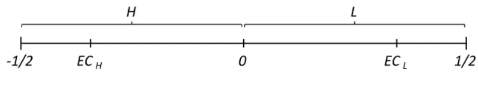
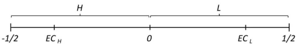
We consider a linear city divided into two jurisdictions with the same size. Each jurisdiction has an employment center where agents can work. The total number of residents of the city is normalized to1, as well as the city size, with extreme points of the segment -1/2 and 1/2. Inhabitants are uniformly distributed across the city and cannot choose their residence location. Each agent is indexed by his residence place, x.

(16)

n(x) = 1 and N(x) =x+1₂

Since the two jurisdictions have the same size and residents are uni-formly distributed, both have the same number of inhabitants,N¯ = 1/2. The median resident of each jurisdiction coincides with the geographic center of the jurisdiction, i.e., mH =−1/4 andmL= 1/4. The

employ-ment centers are assumed to be symmetrically located inγ and−γ and located outwards from the median resident (γ > 1/4). This opens up the possibility for a majority of residents of one jurisdiction to commute to the other one.

Firms located at the employment centers produce an homogeneous good according to a linear technology Yi =αiNi, whereYi is the output

andNi is the number of workers in jurisdictioni.6 The two jurisdictions

have unequal productivities. We use H to denote the high-productivity jurisdiction and L for the low-productivity one, withαH > αL.

H L

‐1/2 EC_H 0 EC_L 1/2

Figure 1.1: The City

The government of each jurisdiction collects a head tax (Ti) paid by

all its residents and, possibly, an ad-valorem source-based tax on wages (τi) paid by all workers in the employment center of jurisdiction i to

ﬁnance a public good budgetGi.7

The local government budget constraint is therefore

Gi =TiN¯ +αiτiNi

whereαi is the gross wage earned by workers in the employment center

of jurisdictioniand Ni is the number of workers in that jurisdiction.

Agents support a per-mile commuting costcand can choose to which employment center they want to commute (i.e., where they want to work). Commuting to the jurisdiction where they do not live is, there-fore, more costly than commuting to the one where they live since the

6

As stated in Peralta (2007) the assumption of a linear technology is not essential and the obtained results would remain unchanged if we introduce perfectly mobile capital in the model with a constant returns to scale production function.

7

(17)

distance they must travel is higher. Each individual provides one unit of labor and pays a wage tax at the source so that the net wage earned by an individual working in j is ωj = αj(1−τj). All agents have a

revenueW from other sources which is assumed to be high enough such that everyone can always pay his tax bill. Agents get utility both from private consumption and from the public good provided.

We follow Peralta (2007) and Braid (2000) and assume a quasi-linear utility function; however, diﬀerently from those authors, we allow indi-viduals to enjoy both the public goods of their residence and work place. The utility enjoyed by individualx, who lives iniand works injis given by:

uij(x;τ;Gi;Gj) =ωj−Ti+W−c|x−ECj|+(1−k)υ(Gi)+kυ(Gj) (1.1)

i, j =H, L

where ECj is the location of the employment center where the agent

chooses to work (γ or ₋γ), Gi is the public good provided in the

juris-diction where he lives,Gj is the public good provided in the jurisdiction

where he works and υ(G) is an increasing concave function. We some-times use the functionυ(G) =√Gto illustrate some of our results. The intensity of the spillover eﬀect due to having individuals deriving utility from the public goods provided in both jurisdictions is measured by the constantk, where0_≤k_≤1. Whenk_≤1/2,Gi is more important than

Gj, i.e., agents care more for the public good provided in the jurisdiction

where they live than for the one provided in the jurisdiction where they work.8

Again, notice that this is not the standard spillover eﬀect we can ﬁnd in the literature. In our case agents only get utility from the public good provided in the other jurisdiction if they decide to work there, i.e., the spillover is endogenous. When they decide the working location they are also choosing the public good mix they want to consume.

1.2.1 The choice of the workplace

An agent works in the jurisdiction where he lives if uii(x;τ;Gi;GH)−

uij(x;τ;Gi;GL)≥0 and commutes to the other jurisdiction otherwise.

8

(18)

Looking at this utility diﬀerence we can calculate the marginal in-terjurisdictional commuter, denoted xˆ. From (1) we can see that the diﬀerence between the utility obtained working in H and the one ob-tained by working in L is:

uiH−uiL=



   

   

ωH−ωL+ 2γc+k[υ(GH)−υ(GL)] if x≤ −γ

ωH−ωL+ 2xc+k[υ(GH)−υ(GL)] if −γ < x < γ

ωH−ωL−2γc+k[υ(GH)−υ(GL)] if x≥γ

If uiH(x;τ)−uiL(x;τ) is positive the agent chooses to work in H,

otherwise he chooses to work in L. Note that for _|x_| > γ the utility diﬀerence is independent from x which means that if one agents that lives between the employment center of a jurisdiction and its outer limit wants to commute to the other one, every agent wants to do the same. We assume away such non-interesting cases and focus on the situation where₋γ < x < γˆ . The marginal ij-commuter xˆ is the one indiﬀerent between working in H or L, therefore

ˆ

x= ωH −ωL+k[υ(GH)−υ(GL)]

2c (1.2)

This marginal interjurisdictional commuter xˆ deﬁnes a commuting equilibrium where allx <xˆ work in H and all x >xˆ work in L.

1.3 First Best

We now compute the utilitarian ﬁrst best to use as a benchmark for the tax competition equilibrium analysis, i.e., the decision of a benevolent social planner that chooses the wage taxes, the residence taxes, the level of public good provided in each jurisdiction and allocates workers to an employment center so that overall utility is maximized.

The planner thus faces an overall budget constraint such that the provision of public goods must be fully paid by the wage and head taxes, i.e.,

GH+GL=τHαH N¯+ ˆx

+τLαL N¯ −xˆ

+ ¯N(TH+tL) (1.3)

(19)

utility of all inhabitants of jurisdiction H (UH) and of all inhabitants of

jurisdiction L (UL), subject to the budget constraint (3), by choosingxˆ,

GH and GL. It is never optimal to have H-residents commuting to L

since their commuting cost is higher than if they work in H and their productivity is lower. Therefore, we can only have L residents commuting to H, i.e., xˆ_≥0, which allow us to calculateUH andULas:

UH =

Z 0

−12

uHHdx (1.4)

UL=

Z xˆ

0

uLHdx+

Z 1₂

ˆ

x

uLLdx (1.5)

Denoting by Ci the total commuting costs of all the residents of

jurisdictioni, we have

CH =c

" Z ₋γ

−12

(₋γ₋x)dx+ Z 0

−γ

(x+γ)dx

#

=c

1 8+γ

2₋γ

2

(1.6)

CL=c

" Z ₋xˆ

0

(x+γ)dx+ Z γ

ˆ

x

(γ₋x)dx+ Z 1₂

γ

(x₋γ)dx

#

=CH+c xˆ2

(1.7) where the last term inCL is the increase in commuting costs due to the

interjurisdictional commuters which must travel a longer distance. Total utility in each jurisdiction is therefore given by:

UH = ¯N[ωH −TH +W +υ(GH)]−CH (1.8)

UL= ¯N[ωL−TL+W +υ(GL)]−CH + ˆx[ωH −ωL+k∆(υ)]−c xˆ2

(1.9) where∆(υ) =υ(GH)−υ(GL)and k∆(υ) is the impact on utility of the

consumption of the public good provided in jurisdiction H rather the one provided in L to interjurisdictional commuters.

Note that the two last terms ofUL are the gain to L of having

inter-jurisdictional commuters. The novelty of our analysis is reﬂected on the term∆(υ) =υ(GH)−υ(GL)generated by the spillover eﬀect of the

(20)

in the level of public goods provided (weighted by k since they always get utility(1₋k) fromGL, the public good provided in the jurisdiction

where they live).

Solving the social planner problem presented previously we can ig-nore the choice of the wage and head tax. Since the planner can allocate the workers to any of the employment centers, the fiscal instruments used to finance the public good is not relevant. The only thing that must be ensured is that the budget constraint is satisfied with these taxes. We can then assume τi = 0 and finance the public goods exclusively with

the head (lump-sum) taxes, which ensures the absence of any type of interjurisdictional transfers.9

Remember that the purpose of the calcu-lation of the ﬁrst best is to use it as a benchmark to compare with the tax competition equilibrium and so we want to keep it as neutral as possible.

The relevant ﬁrst order conditions are therefore:

∂()

∂xˆ = 0⇔xˆ

o ₌ αH −αL+k∆(υ)

2c (1.10)

∂()

∂GH

= 0_⇔υ′₍_Go H)

1 2 + ˆxk

= 1 (1.11)

∂()

∂GL

= 0_⇔υ′₍_Go L)

1 2−xkˆ

= 1 (1.12)

Equation (10) gives the optimal interjurisdictional commuterxˆo_{, which}

results from the trade-oﬀ between commuting costs and productivity gains and the public good level.10

Equations (11) and (12) express the Samuelson condition for the op-timal provision of public goods. Since GH provides k-weighted utility

also toxˆresidents of L, the marginal beneﬁt ofGH is higher than

with-out the spillover (reﬂected by the termxkˆ ) while the inverse applies to

GL.

1.4 The Equilibrium with Residence Taxes

Having calculated the conditions that deﬁne the ﬁrst best, we can now compute the tax competition equilibrium and compare it to the

utili-9

As pointed in Peralta (2007).

10

(21)

tarian optimum. In this section we assume that a government elected by majority rule in each jurisdiction decides the taxes and public goods levels. The elected policy is the one preferred by the median voter of each jurisdiction which in our model coincide with the median resident, i.e.,mH =₋1/4and mL= 1/4.

In this section we compute the tax competition equilibrium when local governments only have access to the residence tax, Ti. We can

then use this equilibrium to compare with the one resulting from the use of a distortive wage tax combined with a lump-sum tax, which is computed in the next section.

Each local government maximizes the utility of the median voter by choosingGi andTi subject to the commuting equilibrium, xˆ, in (2) and

to the budget constraint of the jurisdiction whenτ = 0, i.e., Gi= ¯N Ti.

For the utility of the median voter we must separate the case where he commutes to the other jurisdiction from the case where he commutes to the employment center of his own jurisdiction. We present two cases, depending on whether the median voter of L works in L or H. While we cannot ensure in general that H does not commute to region L, we show in the appendix that this can never happen withυ(G) =√G. The intuition for this resides on the fact that the gross wage earned in L is lower and the traveled distance bymH is much higher than if he decides

to work in the employment center of H. For the median voter of L it can make sense to commute to H thanks to the increase in productivity.

The median voter of H thus enjoys an utility of:

umH =αH+W −TH −c

−1₄+γ

+υ(GH)

For the median voter of L we must separate the case where he works in L from the case where he commutes to work in H. In the former case, since the only public good he consumes isGL, we can compute his utility

as:

umL=αL+W −TL−c

γ₋1

4

+υ(GL)

However, if he decides to work in H he gets utility both from GL

(weighted by1₋k) andGH (weighted byk) and his utility is, therefore,

given by:

umL =αH+W −TL−c

1 4 +γ

(22)

1.4.1 Median voter of L works in L

Let us ﬁrst assume that the median voter of L works in the employment center of L, which happens whenx <ˆ 1/4. Solving the utility maximiza-tion problem for mH andmL we have the equilibrium levels ofGH and

GLimplicitly deﬁned by:

υ′₍_G∗

H) = 2 (1.13)

υ′₍_G∗

L) = 2 (1.14)

These conditions express the usual equality between marginal beneﬁt and marginal cost. Since the population mass of each jurisdiction is 1/2, the marginal cost borne by the median voter to provide an additional unit of public good is 2.

If we compare the tax competition equilibrium obtained with the ﬁrst-best we can state the following proposition:

Proposition 1: In the tax competition equilibrium where only the

resi-dence tax is available and both median voters work in their own jurisdic-tions:

(i) The local public good in jurisdiction H is underprovided and the one in jurisdiction L is overprovided;

(ii) There is undercommuting of agents.

Proof. See appendix.

The median voter of H does not take into account the spillover eﬀect of the public good provided in H on the L-residents that commute to his jurisdiction and, therefore, considers a lower marginal beneﬁt ofGH

when compared to the ﬁrst-best. This leads to a situation of underpro-vision of this public good. Similarly, the median voter of L does not consider that a fringe xˆ of the residents of L commute to H and, thus, get utility fromGL weighted by k, leading to overprovision ofGL.

Since only the residence tax is being used agents decide their work place considering the gross wage earned and the public good provided in each jurisdiction. Knowing thatGH is underprovided, jurisdiction H

is less attractive than in the ﬁrst-best solution, while jurisdiction L is more attractive due to the overprovision of GL. Therefore, the number

(23)

From the ﬁrst order conditions (13) and (14) we get that the equi-librium levels of public goods are the same in both jurisdictions:

υ′₍_G∗

H) =υ′(G∗L) = 2⇔G∗H =G∗L

Thus, the marginal interjurisdictional commuter is

ˆ

x∗ ₌ αH −αL

2c

Since the median voter of L works in L,

ˆ

x∗₌ αH−αL

2c <

1

4 ⇔αH −αL<

c

2

Therefore, this is the condition that guarantees that the equilibrium exists.

1.4.2 Median voter of L works in H

If the median voter of L works in H he earns gross wage αH and gets

utility from public goods provided by both jurisdictions. For the median voter of H everything remains the same, thus GH is implicitly deﬁned

by (13). The key change for mL is that the utility enjoyed thanks to

the public good provided in his own jurisdiction is weighted by(1₋k), henceGL is implicitly deﬁned by:

(1₋k)υ′₍_G∗

L) = 2 (1.15)

The level of public good provided in jurisdiction L is therefore lower than in the previous case since the marginal beneﬁt of GL to mL is

smaller.

This allows us to establish the following result.

Proposition 2: In the tax competition equilibrium where only the

resi-dence tax is available and both median voters work in the high-productivity jurisdiction, both local public goods are underprovided.

(24)

H he does not take into consideration that part of the residents in L get utility υ(GL) from it instead of (1−k)υ(GL), which results in the

underprovision of this public good.

In this case, we may have both under or overcommuting at the tax competition equilibrium. This stems from the fact that both jurisdiction are less attractive than they are in the ﬁrst best solution due to the underprovision of both public goods.

We now check that the equilibrium obtained respects the condition

ˆ

x >1/4, i.e., the median voter of L commutes to H.

Since we are unable to provide general conditions for this, we choose to illustrate it with a particular utility function, υ(G) = √G, thereby showing that this equilibrium is possible.

υ′₍_G

i) =

1 2√Gi

From the ﬁrst order conditions (13) and (15) we get the equilibrium levels forGH and GL

1 2p

G∗

H

= 2_⇔G∗

H =

1 16

1 2p

G∗

L

= 2

1₋k ⇔G

∗

L=

(1₋k)2 16

Thus, the marginal interjurisdictional commuter is

ˆ

x∗ ₌

αH−αL+k

_q

1 16−

q

(1−k)2

16

2c =

αH −αL+k

2

4

2c

For the median voter of L to work in H,

ˆ

x∗ ₌ αH −αL+

k2

4

2c >

1

4 ⇔αH −αL+

k2

4 <

c

2

(25)

1.5 The Tax Competition Equilibrium with

Res-idence and Wage Taxes

We now focus on the tax competition equilibrium attained when local governments can use both the residence (lump-sum) and the wage (dis-tortive) tax.

As a matter of fact, agents are now concerned with the net wage they earn in each employment center rather than the gross wage dictated by their productivity. This means that local governments, when deciding the wage tax level, face a trade-oﬀ between ﬁnancing the public good and reducing the number of interjurisdictional commuters due to the reduction of the net wage in the jurisdiction.

As in the previous framework, each local government maximizes the utility of the median voter by choosing Gi, τi and Ti, subject to the

commuting equilibrium xˆ in (2) and to the budget constraint of the jurisdictionGi = ¯N Ti+τiαiNi.

Remember that Ni is the number of agents working in the

employ-ment center of jurisdictioniso that NH = 1₂ + ˆxand NL= 1₂ −xˆ.

Again, for the utility of the median voter we must separate the case where he commutes to the other jurisdiction from the case where he commutes to the employment center of his own jurisdiction. For the median voter of H, and as we did in the previous section, we know that he never commutes to jurisdiction L since the gross wage is lower and the traveled distance is much higher than if he decides to work in the employment center of H. For the median voter of L it can make sense to commute to H thanks to the increase in productivity. Therefore, the median voter of H enjoys an utility of:

umH = (1−τH)αH +W −TH−c

−1₄ +γ

+υ(GH)

For the median voter of L, his utility when he works in his own jurisdiction is given by:

umL= (1−τL)αL+W −TL−c

γ₋1

4

+υ(GL)

If he decides to work in H he gets utility both fromGL(weighted by

1₋k) andGH (weighted byk) and his utility is, therefore, given by:

umL= (1−τH)αH +W −TL−c

1 4+γ

(26)

1.5.1 Median voter of L works in L

Let us ﬁrst assume that the median voter of L works in the employment center of L, which happens whenx <ˆ 1/4. Solving the utility maximiza-tion problem for mH andmL we have the equilibrium levels ofGH and

GLimplicitly deﬁned by:

υ′₍_G∗∗

H) = 2

1₋τHαH

k

2cυ

′₍_G∗∗

H)

(1.16)

υ′₍_G∗∗

L) = 2

1₋τLαL

k

2cυ

′₍_G∗∗

L)

(1.17) These conditions express the usual equality between marginal ben-eﬁt and marginal cost. Note that the marginal cost is aﬀected by the term τiαi(k/2c)υ′(Gi), which is the impact of the level of public good

on the government budget due to interjurisdictional commuters, whose choice of working place is driven by public good provision. This means that increasing the provision of the public good increases the number of workers subject to the wage tax, aﬀecting the cost borne by the median voter.

If we now look at the ﬁrst order conditions that deﬁne reaction func-tions on τH and τL and combine them we obtain the equilibrium levels

of the wage taxes given by:11

τ∗∗

H =

αH −αL+k∆∗∗(υ)

3αH

τ∗∗

L = −

(αH −αL)−k∆∗∗(υ)

3αL

which yields the equilibrium marginal interjurisdictional commuter:

ˆ

x∗∗₌ αH −αL+k∆∗∗(υ)

6c

With these expression we can show that, in equilibrium, τ∗∗

H αH >

τ∗∗

L αL and G∗∗H > G∗∗L since the opposite relations are ruled-out by the

conditionxˆ∗∗_>₀_.12

The characterization of the tax competition equilibrium is provided in the following proposition:

11

The full first order conditions can be found in the appendix.

12

(27)

Proposition 3: In the tax competition equilibrium where both the resi-dence and the wage taxes are available and both median voters work in their own jurisdictions:

(i) The wage is taxed in H and subsidized in L;

(ii) The local public good in jurisdiction H is underprovided while the one in jurisdiction L is overprovided;

(iii) There is undercommuting of agents.

The result that region H taxes wages while region L subsidizes them is also obtained by Peralta(2007): H residents are exporting part of their tax burden to the interjurisdictional commuters from region L using the wage tax and since the median voter of L works in L, he uses the head tax to impose a higher tax burden to the interjurisdictional commuters, which does not receive the wage subsidy. What we are seeing is a transfer of income from the interjurisdictional commuters to everyone else.

As for the provision of public goods, agents in H have a marginal cost of GH lower than those in L. Since both the median voters of H

and L are exporting part of the tax burden to the L interjurisdictional commuters we have two eﬀects: for H residents,GH is less expensive due

to the tax export and due to the fact that by increasingGH the number

of such commuters increase, which makes it even less expensive; for the median voter of L increasing GL decreases the number of commuters,

which increases the marginal cost.

Comparing the levels of public good provided in each jurisdiction with the ﬁrst-best solution, we reach an intuitive underprovision of the public good of jurisdiction H and overprovision of the one of jurisdiction L, as in the previous section.

All these distortions lead to undercommuting. This is easily ex-plained by the fact that jurisdiction H is less attractive, while jurisdiction L is more attractive than in the ﬁrst best case. A lower net wage earned in the employment center of H (due to the positive wage tax τH) and a

lower level ofGH make jurisdiction H not so appealing while the opposite

happens for L (with subsidized wages and higher provision of GL).

1.5.2 Median voter of L works in H

(28)

the problem for the median voter of H remains unchanged, and GH is

implicitly deﬁned by (16). However, formL his utility is now given by:

umL= (1−τH)αH +W −TL−c

1 4+γ

+ (1₋k)υ(GL) +kυ(GH)

Recall that the diﬀerence to the previous case is that the median voter of L gets (1₋k)-weighted utility from GL and k-weighted utility

fromGH, the public good provided where he works.

The decision on GLis given by:

(1₋k)υ′₍_G∗∗

L) = 2

1₋τLαL

k

2cυ

′₍_G∗∗

L)

The marginal beneﬁt of GLfor the median voter of L is weighted by

(1₋k) instead of 1, since he works in H and therefore gets k-weighted utility from GH. The expression for the marginal cost is the same as

before.

Regarding the wage taxes, combining the ﬁrst order conditions from the problems of mH and mL we get the following equilibrium

expres-sions:13

τ∗∗

H =

αH−αL+c+k∆∗∗(υ)

3αH

τ∗∗

L =

2c₋(αH−αL)−k∆∗∗(υ)

3αL

which yields the equilibrium marginal interjurisdictional commuter:

ˆ

x∗∗₌ αH −αL+k∆∗∗(υ)

6c +

1 6

The next proposition characterizes the tax competition equilibrium:

Proposition 4: In the tax competition equilibrium where both the

resi-dence and the wage taxes are available and both median voters work in the high-productivity jurisdiction:

(i) The wages are taxed in H and in L;

(29)

In this situation no jurisdiction is willing to subsidize wages. The median voter of L is not willing to subsidize the wage in L due to the fact that he is not working in that jurisdiction. Since he is now one of the interjurisdictional commuters he wants to use τL to ﬁnance the budget

of L because he is not subject to such tax.

As for the provision of public goods, the intuition is basically the same as in the previous case, with the additional fact that on the choice ofGLthe marginal beneﬁt for mL is now smaller since it is weighted by

(1₋k).

We can still show thatGH is underprovided, but regarding the public

good of jurisdiction L and the number of commuters we cannot be sure how the equilibrium levels compare with the ﬁrst best. We can only say that if we have overprovision of GL we have undercommuting

(jurisdic-tion L is more attractive than it should) and if we have overcommuting we have underprovision ofGL.14 However, the opposite implications are

not valid.

The intuition for the underprovision ofGH is the same as before, but

now forGLall we know is that, comparing to the case where the median

voter of L works in L and we are able to say that it is overprovided, the marginal beneﬁt is now lower due to the (1₋k) weight. This implies that theGL level chosen bymL is lower, but we cannot be sure if this

reduction is such that it is not overprovided: it can be above the ﬁrst best or it can be bellow the ﬁrst best. This uncertainty about the un-der or overprovision of GL extends to the commuting level since it is a

determinant of the desirability of working in L.

1.6 Only Residence Tax vs. Residence and Wage

Taxes

In this section we compare the tax competition equilibrium obtained when local governments only use the lump-sum head tax to the one when both the lump-sum head tax and the distortive wage tax are used. Following the structure of the previous sections, we ﬁrst focus on the case where the median voter of L works in L. Comparing the two tax competition equilibria we achieve asecond-best result induced by the use of the distortive tax:

14

(30)

Proposition 5: When both median voters work in their own jurisdic-tions, the use of the distortive tax enhances the provision of the public goods vis-a-vis the case where only the lump-sum tax is used.

As a matter of fact, the proof shows that:

GOH > G∗∗H > G∗H

GOL < G∗∗L < G∗L

The distortion introduced by the wage tax partially offsets the inef-ficiency created by the tax competition equilibrium due to the spillover effect of the public goods to the interjurisdictional commuters. This is a typicalsecond-best result where the introduction of two distortions (the wage tax and the inter-jurisdictional externalities) improves upon the case where only one distortion is present. The tax export generated by the wage tax on H reduces the marginal cost to the policy-maker in H, thus leading him to provide a higher level ofGH, thus getting closer to

the optimal provision. The reverse applies to L where the overprovision is reduced by the introduction of the wage subsidy that increases the cost of provision tomL.

When we look at the case where the median voter of L works in H the achieved result is not so strong:

Proposition 6: When the median voter of H works in H while the

median voter of L is an interjurisdictional commuter, the use of the dis-tortive tax increases the level of public goods provided in both jurisdictions vis-a-vis the case where only the lump-sum tax is used.

Proof. See appendix. The proof shows that:

GO_H > G∗∗

H > G∗H

G∗∗

L > G∗L

(31)

underprovision to overprovision, since we are not sure of the comparison between G∗∗

L and GoL as seen in the previous section.

1.7 Conclusion

This paper introduces commuting-related spillovers in a duo-centric lin-ear city where local governments provide public goods and agents choose in which region they want to work.

We show that in the tax competition equilibrium the public goods provided in the most productive region is always underprovided and the one provided in the less productive region can be under or overprovided. Furthermore, we showed that the use of the distortive tax tends to be preferred to the single use of a lump sum tax in terms of the provision of the public goods as it partially oﬀsets the distortion introduced by the endogenous spillover eﬀect.

Since the results were obtained using very general assumptions they are quite robust since they do not depend on explicit functional forms for, e.g.,υ(Gi). The two kinds of taxes considered are also currently used

(32)

1.8 Appendix

Proof of Proposition 1.

(i) υ′₍_Go

H)−υ′(G∗H) = 1+2ˆ2xo_k − 2₁ < 0 since 1 + 2ˆxok > 1. Thus,

Go

H > G∗H.

υ′₍_Go

L) −υ′(G∗L) = 1−2ˆ2xo_k − 2₁ > 0 since 1−2ˆxok < 1. Thus

Go

L< G∗L

(ii) xˆo₋_x_ˆ∗₌ αH−αL+k[υ(GoH)−υ(GoL)]

2c −

αH−αL+k[υ(G∗H)−υ(G∗L)]

2c

Since Go

H > G∗H and GoL< G∗L,xˆo−xˆ∗>0⇔xˆo>xˆ∗

For GH please check the proof of proposition 1 as the problem is the

same.

υ′₍_Go

L)−υ′(G∗L) = 1−2ˆ2xo_k−₁₋2_k

Using the fact thatxˆo_∈ 0;1₂

, we can state that1₋k <1₋2ˆxok, i.e.,

υ′₍_Go

L)−υ′(G∗L)<0. Thus,GoL> G∗L

(i) τ∗∗

H =

αH−αL+k[υ(G∗∗H)−υ(G∗∗L)]

3αH

Therefore,τ∗∗

H >0since G∗∗H > G∗∗L.

τ∗∗

L =

−(αH−αL)−k_[υ(G∗∗

H)−υ(G∗∗L)]

3αL

Therefore,τ∗∗

L <0since G∗∗H > G∗∗L

(ii) υ′₍_Go

H)−υ′(G∗H∗) = 1+2ˆ2xo_k−_1+2ˆ2_x∗∗_k

Thus, Go

H > G∗∗H since xˆo>xˆ∗∗

υ′₍_Go

L)−υ′(G∗∗L) = 1−2ˆ2xo_k− ₁₋_2ˆ2_x∗∗k

Thus, Go

L< G∗∗L since xˆo>xˆ∗∗

(iii) xˆo₋_x_ˆ∗∗₌ αH−αL+k[υ(GoH)−υ(G o L)]

2c −

6c

Therefore,xˆo_>_x_ˆ∗∗ _since _Go

H > G∗∗H and GoL< G∗∗L

(33)

(i) τ∗∗

H α∗∗H = 3c + 2c xˆ∗∗−16

Since xˆ∗∗_∈ 1

4;12

,τ∗∗

H >0

τ∗∗

L α∗∗L = 23c−2c xˆ∗∗− 16

Sincexˆ∗∗_∈ 1

4;12

,τ∗∗

L α∗∗L ∈ 0;12

, which allow us to state τ∗∗

L >0

(ii) For GH please check the proof of proposition 3 as the problem is

the same.

υ′₍_G∗

H)−υ′(G∗∗H) = 2− 1+2ˆ2x∗∗

Since 1 + 2ˆx∗∗ _> ₁_{, we can state that} _υ′₍_G∗

H) −υ′(G∗∗H) > 0, i.e.,

G∗

H < G∗∗H

υ′₍_G∗

L)−υ′(G∗∗L) = 21− 1−2ˆ2x∗∗

Since1₋2ˆx∗∗_<₁_{, we can state that}_υ′₍_G∗

L)−υ′(G∗∗L)<0, i.e.,G∗L> G∗∗L

υ′₍_G∗

H)−υ′(G∗∗H) = 12 −1+k(2ˆx2∗∗₋1 3)

Sincexˆ∗∗_∈ 1

4;12

, we can state that1 +k 2ˆx∗∗₋1

3

>1, thus allowing to conclude thatυ′₍_G∗

H)−υ′(G∗∗H)>0, i.e.,G∗H < G∗∗H

υ′₍_G∗

L)−υ′(G∗∗L) = 1−2k−₁₊k₍42 3−2ˆx∗∗)

Sincexˆ_∈ 1₄;1₂

, we can state that 1 +k 4₃₋2ˆx∗∗

>1₋k, thus allow-ing to conclude thatυ′₍_G∗

L)−υ′(G∗∗L)>0, i.e., G∗L< G∗∗L

The median voter of H is not willing to work in L in section 4.

If the median voter of H commutes to L, x <ˆ ₋1/4 and the local gov-ernment in H:

max

Gi,Ti

umH =αL+W −TH−c

1 4 +γ

+ (1₋k)pGH +k

p

GL

s.t.xˆ= αH −αL+k

√

GH −√GL

2c

GH =

(34)

FOC:

1 2√GH

= 2

1₋k ⇔

p

G∗

H =

1₋k

4

The ﬁrst order condition inGLis the same as (14) which leads to√GL=

1/4.

The commuting equilibrium is therefore deﬁned by:

ˆ

x= αH −αL+k

1−k

4 −14

2c

and sincek_∈(0; 1)

ˆ

x_∈ αH −αL−

1 4

2c ;

αH −αL

2c

!

>₋1

4

Thus, and as expected, it is impossible to have the median voter of H commuting to L since he would bear a higher commuting cost and earn a lower wage.

FOC of the utility maximization problems is section 5.1.

∂UmH

∂GH = 0⇔ −2 h

1₋τHαH_∂G∂xˆ

H i

+υ′₍_G_H_{) = 0}_{, which after}

straightfor-ward computations leads toυ′₍_G∗∗

H) = τHα2Hck+c.

∂UmH

∂τH = 0 ⇔ −αH −2 h

−αH 1₂ + ˆx

+τHαH_∂τ∂xˆ_H

i

= 0, which after straightforward computations leads toτ∗∗

H =

αH−(1−τL)αL+k∆(υ)

2αH

∂UmL

∂GL = 0⇔ −2 h

1₋τLαL_∂G∂ˆx_L

i

+υ′₍_G

L) = 0, which after some algebra

results inυ′₍_G∗∗

L) = τLα2Lck+c

∂UmL

∂τL = 0⇔ −αL−2 h

−αL 1₂−xˆ−τLαL_∂τ∂ˆx

L i

= 0, which after some algebra results inτ∗∗

L =

αL−(1−τH)αH+k∆(υ)

2αL

Combining the two reaction functions on the wage tax we get:

τ∗∗

H =

3αH

τ∗∗

L =

−(αH−αL)−k_[υ(G∗∗

H)−υ(G∗∗L)]

(35)

Proof that τ∗∗

HαH > τL∗∗αL and G∗∗H > G∗∗L in section 5.1.

τ∗∗

HαH =

αH−αL+k(υ(G∗∗_H)−υ(G∗∗

L))

3

τ∗∗

L αL=

−(αH−αL)−k(υ(G∗∗H)−υ(G∗∗L))

3

τ∗∗

HαH−τL∗∗αL= 2₃(αH −αL+k[υ(G∗∗H)−υ(G∗∗L)])

If τ∗∗

HαH > τL∗∗αL, G∗∗H > G∗∗L, thus meaning that, τH∗∗αH > τL∗∗αL and

ˆ

x∗∗_>₀, which is ok.

If τ∗∗

H αH < τL∗∗αL, k[υ(GL∗∗)−υ(G∗∗H) > αH −αL, thus implying that

ˆ

x∗∗_<₀, which is impossible.

FOC of the utility maximization problems in section 5.2.

The FOC onUmH are the same as in section 5.1.

υ′₍_G∗∗

H) = 2 c τHαHk+c

τ∗∗

H =

αH−(1−τL)αL+k∆(υ)

2αH

ForUmL we have: ∂UmL

∂GL = 0 ⇔ −2 h

1₋τLαL_∂G∂xˆ_L

i

+ (1₋k)υ′₍_G_L_{) = 0}_{, which results in}

υ′₍_G∗∗

L) = τLαLk2+(1c −k)c ∂UmL

∂τL = 0 ⇔ 2 h

αL 1₂ −xˆ

+τLαL_∂τ∂xˆ_L

i

= 0, which results in τ∗∗

L = c+αL−(1−τH)αH−k∆(υ)

2αL

Combining the two reaction functions on the wage tax we get:

τ∗∗

H =

c+(αH−αL)+k[υ(G∗∗H)−υ(G∗∗L)]

3αH

τ∗∗

L =

2c−(αH−αL)−k[υ(G∗∗

H)−υ(G∗∗L)]

3αL

Proof that, in section 5.2,

(i) Overprovision of GL implies undercommuting of agents;

(ii) Overcommuting of agents implies underprovision of GL.

υ′₍_Go

L)−υ′(G∗∗L) = 1−2ˆ2xo_k− ₁ 2

−2ˆx∗∗_k₋2

3k

(36)

the denominators:

[1₋2ˆxo_k_]₋

1₋2ˆx∗∗_k₋2

3k

= 2k₁

3−(ˆxo−xˆ∗∗)

Overprovision of GL, i.e., Go_L < G∗∗_L, implies that υ′(Go_L) > υ′(G∗∗_L).

Therefore,2k₁

3 −(ˆxo−xˆ∗∗)

<0. For this to be true, xˆo _>_x_ˆ∗∗_.

Overcommuting of agents, i.e.,xˆo_<_x_ˆ∗∗_{, implies that}₂_k₁

3 −(ˆxo−xˆ∗∗)

>

0. Therefore,υ′₍_Go

L)< υ′(G∗∗L), i.e., GoL> G∗∗L

(37)

Chapter 2

Endogenous asymmetric

transportation costs and the

impact of toll usage

0

(38)

2.1 Introduction

In the last decades several cities worldwide implemented tolls paid by drivers who want to drive in the city center during working days be-tween early morning and late afternoon. Singapore was the first city to effectively implement a congestion pricing scheme - the Singapore Area Licensing Scheme - in 1975, based on paper licenses; this scheme was later replaced by an electronic charging scheme - the Eletronic Road Pricing (ERP). An impact of the successes and shortcomings of the Singapore road pricing can be found in Phang and Toh (2004). London introduced in 2003 a congestion charge which is levied electronically on vehicles trav-eling on the London Congestion Charge Zone (CCZ), which results have been analyzed for example by Prud’homme and Bocarejo (2005), Leape (2006), Givoni (2011) or Dudley (2013). Stockholm implemented in 2007 the Stockholm Congestion Tax which is levied electronically on vehicles entering and exiting central Stockholm. Milan charges vehicles traveling on the traffic restricted zone (ZTL) with a scheme which started in 2008 with the name “Ecopass" and then took the name “Area C" in 2012. Gothemburg implemented in 2013 a toll similar to the one charged in Stockholm.

Although the main reasons invoked to charge these city tolls are the reduction of congestion and environmental concerns, the revenue levied with the tolls is usually directed to the operation, maintenance, and construction of transportation infrastructure. For example, the London Congestion Charge is one of the sources of revenue of Transport for Lon-don, having generated a revenue of £222 million in 2013 (about 5% of the total revenue, which is mainly composed of public transportation fares, according to the 2013 Transport for London Annual Report). But besides the cases where the main argument behind a toll is congestion, many tolls are charged with the sole purpose of ﬁnancing the expen-ditures generated by an infrastructure, e.g., a highway, a bridge or a tunnel. In Portugal, almost all highways are fully (or at least partially) tolled. In Lisbon, the two available bridges that can be crossed by trav-elers arriving from Tagus river south bank are tolled, and the proceeds are used to fund the maintenance and operation of the bridges.

(39)

Census 2011), while the average time taken to travel to work in cen-tral London was, in 2012, of 54 minutes (UK Department for Transport annual publication “Transport Statistics Great Britain" 2013). These facts put pressure on local governments to improve the transportation infrastructure in order to reduce the transportation costs for their vot-ers (monetary cost and/or time spent in travels), while also meaning that commuters use the transportation infrastructure of more than one jurisdiction. Therefore, whenever a local government improves the trans-portation infrastructure, it is serving all agents using that infrastructure, thus generating positive spillovers to the residents of nearby cities.

Spillovers are, thus, generated by commuting from one region to an-other, making agents enjoy public goods in both the municipality where they live and where they work.1

In this paper we look at the impact of local level ﬁscal decentralization on the provision of public goods that determine transportation cost in a framework where agents commute. We may consider several types of local governments, from jurisdictions in one city to neighboring cities or even states, as long as it is expectable that agents commute from one to the other.

The autonomy of local governments regarding tax collection is far from being homogeneous. Diﬀerent local governments have access to diﬀerent types of taxes, e.g., residence-based wealth or income taxes, source-based income taxes, or “hybrid” taxes. 2

These taxes are usually combined with grants or transfers from the central governments to form the total local budget.

Tolls to have access to the city center are in practice very close to the “hybrid" taxes used, for example, in Kansas City, St. Louis, Wilmington, Detroit, New York City or Philadelphia (Braid, 2009). These “hybrid" taxes are characterized by the fact that all central city residents are taxed at a rate, irrespective of where they work, while residents in the suburbs who work in the central city can be taxed at a different rate. This is precisely the effect of a toll at the entrance of a city or jurisdiction: while the residents are not subject to its payment, the residents in the adjoining cities (or in the suburbs) must pay it, therefore resulting in different amounts being charged to each type of worker.

The contribution of this paper is the introduction of endogenous and asymmetric transportation costs in the framework of a linear city allow-ing, simultaneously, to study the impact of charging a toll on the

pro-1

Unlike the case of the exogenous spillover effect considered, e.g., in Besley and Coate (2003) that follows the traditional Oates’s spillover effect.

2

(40)

vision of transportation infrastructure on cities. The linear city model is the one used by, e.g., Braid (2000) and Peralta (2007) to tackle inter-jurisdictional tax spillovers. The city is divided into two jurisdictions and agents choose where they want to work. Productivity, and thus wages, differ across regions and individuals trade-off the advantages (i.e., wage and working conditions) of a given job against travel costs (distance, time, and money) when choosing their workplace. The travel cost differs from one jurisdiction to the other since it depends on the level of local public good (which can be understood as transportation infrastructure) being provided in each jurisdiction. This formulation implicitly intro-duces a spillover effect on the public good provided on a jurisdiction that provides employment to the residents of the other one. We take the residence of agents as given, assuming independence between residence and working choices. This independence is argued by Wildasin (1986) and supported by empirical evidence provided by Rouwendal and Meijer (2001), Glaeser et al. (2001) and Zax (1991 and 1994).

We take a representative agent who derives utility from both the public good provided in the residence location and in the working place. This means that agents only beneﬁt from the transportation cost result-ing from the public good supplied in the other jurisdiction if they choose to work there. Otherwise they are only interested in the transportation infrastructure provided in their own jurisdiction. We abstract from other forms of interjurisdictional commuting, e.g., for leisure or shopping. A worker uses the transportation infrastructure daily and is therefore much more important.

Our main results are as follows. Firstly, the toll distorts the number of interjurisdictional commuters. However, it may improve the provi-sion of the public good in the high productivity jurisdiction, where the transportation infrastructure is underprovided if funded only by resi-dence taxes, as it decreases the marginal cost faced by the median voter of that jurisdiction. A simulation shows that, even though the provision of the public in the high productivity jurisdiction may be closer to the optimal, the overall utility is decreased by the introduction of the toll due to the reduction of interjurisdictional commuters that it imposes.

(41)

2.2 The Model

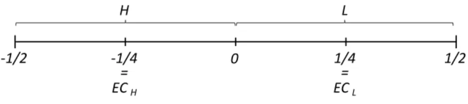
We consider a linear city divided into two jurisdictions with the same size. Each jurisdiction has an employment center where agents can work. The total number of residents of the city is normalized to1, as well as the city size, with extreme points of the segment -1/2 and 1/2. Inhabitants are uniformly distributed across the city and cannot choose their residence location. Each agent is indexed by his residence place, x.

Letn(x) andN(x) denote the density and distribution function, re-spectively, so that

n(x) = 1 and N(x) =x+1₂

Since the two jurisdictions have the same size and residents are uni-formly distributed, both have the same number of inhabitants,_N¯ _{= 1}_/₂_.

The employment centers are assumed to be symmetrically located in the center of each jurisdiction, i.e., −1/4 and 1/4. The maximum travel distance from a point in the jurisdiction and the employment center is, therefore, 1/4. Since we are analyzing the choice of a local public good with impact on the transportation costs, the median voter of each juris-diction is the one that travels the median distance, i.e.,mH =−1/8and

mL= 1/8.3

Firms located at the employment centers produce an homogeneous good according to a linear technology Yi =αiNi, whereYi is the output

andNi is the number of workers in jurisdictioni.4 The two jurisdictions

have unequal productivities. We use H to denote the high-productivity jurisdiction and L for the low-productivity one, withαH > αL.

The government of each jurisdiction collects a head tax (Ti) paid

by all its residents and, possibly, a toll situated at point 0 paid by the interjurisdictional commuters that are arriving at the jurisdiction, to ﬁnance a public goodGi.5

3

As a matter of fact, if we assume that the median voter works in his own juris-diction, there are two agents that travel the same distance from their residence to the employment center: for the high productivity jurisdiction, both the one that stands at−₃_/₈_{and the one that stands at} ₁_/₈_{must travel a distance of}₁_/₈_{, while for the}

low productivity jurisdiction both the agents at1/8and3/8travel the same distance. We can therefore use either one or the other, but if we open the possibility of the median voter to commute to the employment center of the other jurisdiction, only the one that stand at−1/8(in H) or1/8(in L) fit the median distance of 1/8.

4

As stated in Peralta (2007) the assumption of a linear technology is not essential and the obtained results would remain unchanged if we introduce perfectly mobile capital in the model with a constant returns to scale production function and a small region assumption such that f’(k) is given.

5

(42)

H L

0

‐1/2 ‐1/4 1/4 1/2

= =

EC_H EC_L

Figure 2.1: The City

The local government budget constraint is therefore

Gi =TiN¯ +Pi(max(Ni−N¯; 0))

where Pi is the toll collected at the border of jurisdiction i and Ni is

the number of workers in that jurisdiction. Note that the toll is only paid by the interjurisdictional commuter that are arriving at the region, i.e., the number of workers that exceed the residents of that jurisdiction (Ni−N¯); if there is no interjurisdictional commuting towards that region,

the number of workers paying the toll is null.

To travel on each jurisdiction, agents support a per-mile commuting cost ci which depends on the local public good provision in that

juris-diction, i.e.,ci(Gi). Agents can choose to which employment center they

want to commute (i.e., where they want to work). Commuting to the jurisdiction where they do not live is, therefore, more costly than com-muting to the one where they live since the travel distance is higher. Each individual provides one unit of labor and earns a wage ωj = αj

for working in the employment center located in j. All agents have a revenueW from other sources which is assumed to be high enough such that everyone can always pay his tax bill.

Agents get utility from private consumption, following a linear utility function similar to the quasi-linear utility function used by Braid (2000) and Peralta (2007), but where the utility arising from the public good is indirectly captured by the reduction in the transportation cost. Since the transportation cost is not symmetric in the two jurisdictions it is important to write the utility function in two cases: (i) when the agent lives and works in the same jurisdiction, and (ii) when the agent is an interjurisdictional commuter. The utility enjoyed by individual x, who lives and works ini, is given by:

uii(x;Gi) =ωi−Ti+W −c(Gi)|x−ECi|, i, j=H, L (2.1)

where ECi is the location of the employment center (−1/4 or 1/4)

(43)

and c(Gi) is the transportation cost per mile, which depends on the

public good provided in the jurisdiction where the agent lives (Gi).

The utility enjoyed by individual x, who lives in i and works in j

(withi₆=j) is given by:

uij(x;Pj;Gi;Gj) =ωj−Ti+W−c(Gi)|x| −c(Gj)|0−ECj| −Pj , (2.2)

i, j =H, L

where ECj is the location of the employment center where the agent

chooses to work (₋1/4or1/4),c(Gi) is the transportation cost per mile

in the jurisdiction where the agent lives, which depends on the public good provided in that jurisdiction (Gi), c(Gj) is the transportation cost

per mile in the jurisdiction where the agent works, which depends on the public good provided there (Gj), andPj is the toll charged when the

agent enters jurisdiction j.

The transportation cost per mile in each jurisdiction is given byc(Gi),

which is a decreasing convex function, i.e.,

c′

i = ∂G∂ci <0 and c

′′

i = ∂

2_c

∂G2

i

>0

2.2.1 The choice of the workplace

An agent works in the jurisdiction where he lives if

uii(x;P;Gi;GH)−uij(x;P;Gi;GL)≥0

and will commute to the other jurisdiction otherwise. Given that wage in H is greater than the wage in L and the travel distance is higher if the agent decides to commute to the other jurisdiction rather than work on his own jurisdiction, it is possible to show that the tax competition equilibrium never involves commuting from H to L. Therefore, we focus on the choice of the workplace of the agents who live in L.

Computing the utility diﬀerence we can calculate the marginal in-terjurisdictional commuter, denotedxˆ. Using (1) and (2), the diﬀerence between the utility obtained working in H and the one obtained by work-ing in L for a resident on L is:

uiH−uiL=

(

ωH −ωL+1₄(cL−cH)−PH −2xcL if−1₄ < x < 1₄

Tax competition with commuting in asymmetric cities