Search for natural and split supersymmetry in proton-proton collisions at $ \sqrt{s}=13 $ TeV in final states with jets and missing transverse momentum

CERN-EP-2018-003 2018/05/23

CMS-SUS-16-038

Search for natural and split supersymmetry in

proton-proton collisions at

√

s

=

13 TeV in final states with

jets and missing transverse momentum

The CMS Collaboration

∗

Abstract

A search for supersymmetry (SUSY) is performed in final states comprising one or more jets and missing transverse momentum using data from proton-proton colli-sions at a centre-of-mass energy of 13 TeV. The data were recorded with the CMS detector at the CERN LHC in 2016 and correspond to an integrated luminosity of

35.9 fb−1. The number of signal events is found to agree with the expected

back-ground yields from standard model processes. The results are interpreted in the con-text of simplified models of SUSY that assume the production of gluino or squark pairs and their prompt decay to quarks and the lightest neutralino. The masses of bottom, top, and mass-degenerate light-flavour squarks are probed up to 1050, 1000, and 1325 GeV, respectively. The gluino mass is probed up to 1900, 1650, and 1650 GeV when the gluino decays via virtual states of the aforementioned squarks. The strongest mass bounds on the neutralinos from gluino and squark decays are 1150 and 575 GeV, respectively. The search also provides sensitivity to simplified models inspired by split SUSY that involve the production and decay of long-lived gluinos.

Values of the proper decay length cτ0from 10−3to 105mm are considered, as well as

a metastable gluino scenario. Gluino masses up to 1750 and 900 GeV are probed for

cτ0 = 1 mm and for the metastable state, respectively. The sensitivity is moderately

dependent on model assumptions for cτ0&1 m. The search provides coverage of the

cτ0parameter space for models involving long-lived gluinos that is complementary

to existing techniques at the LHC.

Published in the Journal of High Energy Physics as doi:10.1007/JHEP05(2018)025.

c

2018 CERN for the benefit of the CMS Collaboration. CC-BY-4.0 license ∗_{See Appendix B for the list of collaboration members}

1

Introduction

Supersymmetry (SUSY) [1–4] is an extension of the standard model (SM) of particle physics that introduces at least one bosonic (fermionic) superpartner for each fermionic (bosonic) SM particle, where the superpartner differs in its spin from its SM counterpart by one half unit. Supersymmetry offers a potential solution to the hierarchy problem [5, 6], predicts unification of the gauge couplings at high energy [7–9], and provides a candidate for dark matter (DM). Under the assumption of R-parity [10] conservation, SUSY particles are expected to be pro-duced in pairs at the CERN LHC and to decay to the stable, lightest SUSY particle (LSP). The

LSP is assumed to be the neutralinoχe

0

1, a weakly interacting massive particle and a viable DM

candidate [11, 12]. So-called natural SUSY models, which invoke only a minimal fine tuning of the bare Higgs boson mass parameter, require only the gluino, third-generation squarks, and a

higgsino-likeχe

0

1to have masses at or near the electroweak (EW) scale [13]. The interest in

natu-ral models is motivated by the discovery of a low-mass Higgs boson [14–19]. The characteristic signature of natural SUSY production at the LHC is a final state containing an abundance of jets originating from the hadronization of heavy-flavour quarks and significant missing transverse

momentum~pmiss

T .

Split supersymmetry [20, 21] does not address the hierarchy problem—in contrast to natural SUSY models—but preserves the appealing aspects of gauge coupling unification and a DM candidate. In such a model, only the fermionic superpartners, and a finely tuned scalar Higgs boson, may be realized at a mass scale that is kinematically accessible at the LHC. All other SUSY particles are assumed to be ultraheavy. Hence, within split SUSY models, the gluino decay is suppressed because of the highly virtual squark states. For gluino lifetimes beyond a picosecond, the gluino hadronizes and forms a bound colour-singlet state containing the gluino and quarks or gluons [22], known as an R-hadron, before eventually decaying to a quark–

antiquark pair and theχe

0

1. The long-lived gluino can lead to final states with significant~pTmiss

from the undetected χe

0

1 particles and to jets with vertices located a significant distance (i.e.

displaced) from the luminous region of the proton beams. A metastable gluino, with a decay length significantly beyond the scale of the CMS detector, can escape undetected.

This paper presents a search for new-physics processes in final states with one or more

ener-getic jets and significant~pmiss

T . The search is performed with a sample of proton–proton (pp)

collision data at a centre-of-mass energy of 13 TeV recorded by the CMS experiment in 2016.

The analysed data sample corresponds to an integrated luminosity of 35.9±0.9 fb−1[23].

Ear-lier searches using the same technique have been performed in pp collisions at√s =7, 8, and

13 TeV by the CMS Collaboration [24–29]. The data set analysed in this analysis is a factor of 16 larger than that presented in Ref. [29]. The search strategy aims to provide sensitivity to a broad range of SUSY-inspired models that predict the existence of a DM candidate, and the search is used to constrain the parameter spaces of a number of simplified SUSY models [30– 32]. The overwhelmingly dominant background for a new-physics search in all-jet final states resulting from pp collisions is the production of multijet events via the strong interaction, a manifestation of quantum chromodynamics (QCD). Several dedicated variables are employed to suppress the multijet background to a negligible level while maintaining low kinematical thresholds and high experimental acceptance for final states characterized by the presence of

significant~pmiss

T . Signal extraction is performed using additional kinematical variables, namely

the number of jets, the number of jets identified as originating from bottom quarks, and the scalar and vector sums of the jet transverse momenta. The ATLAS and CMS Collaborations

have performed similar searches in all-jet final states at√s=13 TeV, of which those providing

the tightest constraints are described in Refs. [33–35]. This search does not employ specialized reconstruction techniques [36–46] that target long-lived gluinos.

This paper is organized as follows. Section 2 describes the CMS apparatus and the event recon-struction algorithms. Section 3 summarizes the selection criteria used to identify and catego-rize signal events and samples of control data. Section 4 outlines the various software packages used to generate the samples of simulated events. Sections 5 and 6 describe the methods used to estimate the background contributions from SM processes. The results and interpretations are described in Sections 7 and 8, respectively, and summarized in Section 9.

2

The CMS detector and event reconstruction

The central feature of the CMS detector is a superconducting solenoid of 6 m internal diameter, providing a magnetic field of 3.8 T. Within the solenoid volume are a silicon pixel and strip tracker, a lead tungstate crystal electromagnetic calorimeter (ECAL), and a brass and scintillator hadron calorimeter (HCAL), each composed of a barrel and two endcap sections. Forward calorimeters extend the pseudorapidity coverage provided by the barrel and endcap detectors. Muons are detected in gas-ionization chambers embedded in the steel flux-return yoke outside the solenoid. A more detailed description of the CMS detector, together with a definition of the coordinate system used and the relevant kinematical variables, can be found in Ref. [47]. Events of interest are selected using a two-tiered trigger system [48]. The first level, composed of custom hardware processors, uses information from the calorimeters and muon detectors to select events at a rate of around 100 kHz within a time interval of less than 4 µs. The second level, known as the high-level trigger, consists of a farm of processors running a version of the full event reconstruction software optimized for fast processing, and reduces the event rate to less than 1 kHz before data storage. The trigger logic used by this search is summarized in Section 3.

The particle-flow (PF) event algorithm [49] reconstructs and identifies each individual particle with an optimized combination of information from the various elements of the CMS detector. In this process, the identification of the particle type (photon, electron, muon, charged hadron, neutral hadron) plays an important role in the determination of the particle direction and en-ergy. The energy of photons [50] is directly obtained from the ECAL measurement, corrected for zero-suppression effects. The energy of electrons [51] is determined from a combination of the electron momentum at the primary interaction vertex as determined by the tracker, the en-ergy of the corresponding ECAL measurement, and the enen-ergy sum of all bremsstrahlung pho-tons spatially compatible with originating from the electron track. The energy of muons [52] is obtained from the curvature of the corresponding track. The energy of charged hadrons is determined from a combination of their momentum measured in the tracker and the matching ECAL and HCAL energy deposits, corrected for zero-suppression effects and for the response function of the calorimeters to hadronic showers. Finally, the energy of neutral hadrons is obtained from the corresponding corrected ECAL and HCAL energy. The reconstruction tech-niques used by this search are not specialized to target specific experimental signatures (such as displaced jets). The physics objects used in this search are defined below and are summa-rized in Table 1. In the case of photons and leptons, further details can be found in Ref. [29] and references therein.

The reconstructed vertex with the largest value of summed physics object p2_T is taken to be

the primary pp interaction vertex (PV). The physics objects considered are those returned by a jet finding algorithm [53, 54] applied to all charged particle tracks associated with the

ver-tex, and the associated pmiss_T , taken as the negative vector sum of the pT of those physics

ob-jects. Charged particle tracks associated with vertices from additional pp interactions within the same or nearby bunch crossings (pileup) are not considered by the PF algorithm as part

Table 1: Summary of the physics object acceptances, the baseline event selection, the signal and control regions, and the event categorization schemas. The nominal categorization schema is defined in full in Appendix A.

Physics object acceptances

Jet pT>40 GeV,|η| <2.4

Photon pT>25 GeV,|η| <2.5, isolated in cone∆R<0.3

Electron pT>10 GeV,|η| <2.5, Irel<0.1 in cone 0.05<∆R(pT) <0.2 Muon pT>10 GeV,|η| <2.5, Irel<0.2 in cone 0.05<∆R(pT) <0.2 Single isolated track (SIT) pT>10 GeV,|η| <2.5, Itrack<0.1 in cone∆R<0.3

Baseline event selection

All-jet final state Veto events containing photons, electrons, muons, and SITs within acceptance

pmiss_T quality Veto events based on filters related to beam and instrumental effects

Jet quality Veto events containing jets that fail identification criteria or 0.1< fj1

h± <0.95

Jet energy and sums pj1

T>100 GeV, HT>200 GeV, HTmiss>200 GeV

Jets outside acceptance Hmiss

T /pmissT <1.25, veto events containing jets with pT>40 GeV and|η| >2.4

Signal region Baseline selection +

αTthreshold (HTrange) 0.65 (200–250 GeV), 0.60 (250–300), 0.55 (300–350), 0.53 (350–400), 0.52 (400–900) ∆φ∗

minthreshold ∆φ∗min>0.5 (njet≥2),∆φmin∗25 >0.5 (njet=1)

Nominal categorization schema

njet 1 (monojet)

≥2a (a denotes asymmetric, 40<pj2

T<100 GeV)

2, 3, 4, 5,≥6 (symmetric, pj2

T>100 GeV)

nb 0, 1, 2, 3,≥4 (can be dropped/merged vs. njet)

HTboundaries 200, 400, 600, 900, 1200 GeV (can be dropped/merged vs. njet, nb)

H_Tmissboundaries 200, 400, 600, 900 GeV (can be dropped/merged vs. njet, nb, HT)

Simplified categorization schema

Topology (njet, nb) Monojet-like (1∩ ≥2a, 0), (1∩ ≥2a,≥1)

Low njet (2∩3, 0∩1), (2∩3,≥2)

Medium njet (4∩5, 0∩1), (4∩5,≥2)

High njet (≥6, 0∩1), (≥6,≥2)

HTboundaries HT>200 GeV (njet≤3), HT>400 GeV (njet≥4) Hmiss

T boundaries 200, 400, 600, 900 GeV

Control regions Baseline selection +

µ+jets (inverted µ veto) pµ_T1>30 GeV,|ηµ1_{| <2.1,}∆R_{(µ, ji) >0.5, 30<m}

T(~pµT,~pTmiss) <125 GeV

µµ+jets (inverted µ veto) pµ_T1,2>30 GeV,|ηµ1,2_{| <2.1,}∆R_(µ

1,2, ji) >0.5,|mµµ−mZ| <25 GeV Multijet-enriched Sidebands to signal region: H_Tmiss/pmiss_T >1.25 and/or∆φ_min∗ <0.5

of the global event reconstruction. The energy deposit associated with each physics object is corrected to account for contributions from neutral particles originating from pileup interac-tions [55].

Samples of signal events and control data are defined, respectively, by the absence or pres-ence of photons and leptons that are isolated from other activity in the event. Photons are required to be isolated [50] within a cone around the photon trajectory defined by the

ra-dius∆R =

√

(∆φ)2+ (∆η)2 = 0.3, where ∆φ and ∆η represent differences in the azimuthal

angle (radians) and pseudorapidity. Isolation for an electron or muon is a relative quantity,

Irel, defined as the scalar pT sum of all PF particle candidates within a cone around its

tra-jectory, divided by the lepton pT. The cone radius is dependent on the lepton pT, ∆R =

Lorentz-boosted top quarks [56]. Isolated electrons and muons are required to satisfy Irel <0.1 and 0.2, respectively. Electron and muon candidates that fail any of the aforementioned requirements, as well as charged-hadron candidates from hadronically decaying tau leptons, are collectively

labelled as single isolated tracks (SITs) if the scalar pTsum of additional tracks associated with

the PV within a cone ∆R < 0.3 around the track trajectory, relative to the track pT, satisfies

Itrack < 0.1. All isolation variables exclude the contributions from the physics object itself

and pileup interactions [50–52]. The experimental acceptances for photons, electrons, muons,

and SITs are defined by the transverse momentum requirements pT > 25, 10, 10, and 10 GeV,

respectively, and the pseudorapidity requirement|η| <2.5.

Jets are reconstructed from the PF particle candidates, clustered by the anti-kT algorithm [53,

54] with a distance parameter of 0.4. In this process, the raw jet energy is obtained from the sum of the particle candidate energies, and the raw jet momentum by the vectorial sum of the particle candidate momenta, which results in a nonzero jet mass. An offset correction is applied to jet energies to take into account the contributions from neutral particles produced in pileup interactions [55, 57]. The raw jet energies are then corrected to establish a relative

uniform response of the calorimeter in η and a calibrated absolute response in pT. Jet energy

corrections are derived from simulation, and are confirmed with in situ measurements of the energy balance in dijet, multijet, γ+jets, and leptonically decaying Z+jets events [58]. Jets are

required to satisfy pT > 40 GeV and |η| < 2.4. Jets are also subjected to a standard set of

identification criteria [59] that require each jet to contain at least two particle candidates and

at least one charged particle track, and the energy fraction fh± attributed to charged-hadron

particle candidates is required to be nonzero.

Jets can be identified as originating from b quarks using the combined secondary vertex (CSVv2) algorithm [60]. Data samples are used to measure the b tagging efficiency, which is the proba-bility to correctly identify jets originating from b quarks, as well as the mistag probabilities for jets that originate from light-flavour (LF) partons (u, d, s quarks or gluon) or a charm quark. A

working point is employed that yields a b tagging efficiency of≈69% for jets with pT>30 GeV

from tt events, and charm and LF mistag probabilities of≈18 and≈1%, respectively, for

mul-tijet events.

Finally, the most accurate estimator for~p_Tmissis defined as the projection on the plane

perpen-dicular to the beams of the negative vector sum of the momenta of all PF particle candidates in

an event. Its magnitude is referred to as pmiss_T .

3

Event selection and categorization

A baseline set of event selection criteria, described in Section 3.1, is used as a basis for all data samples used in this search. Two additional requirements, described in Section 3.2, are employed to define a sample of signal events, labelled henceforth as the signal region (SR). The categorization of signal events and the background composition are described in Sections 3.3 and 3.4, respectively. Three independent control regions (CRs), comprising large samples of event data, are defined by the selection criteria described in Section 3.5. All selection criteria are summarized in Table 1.

3.1 Baseline selections

Events containing isolated photons, electrons and muons, or SITs that satisfy the requirements summarized in Table 1 are vetoed. The aforementioned vetoes are employed to select all-jet final states, suppress SM processes that produce final states containing neutrinos, and reduce

backgrounds from misreconstructed or nonisolated leptons as well as single-prong hadronic decays of τ leptons.

Beam halo, spurious jet-like features originating from isolated noise patterns in the calorimeter

systems, detector inefficiencies, and reconstruction failures can all lead to large values of pmiss_T .

Such events are rejected with high efficiency using dedicated vetoes [61, 62]. Events are vetoed

if any jet fails the identification criteria described in Section 2. Further, fh± for the highest p_Tjet

of the event, j1, is required to satisfy 0.1< f_hj1± < 0.95 to further suppress beam halo and rare

reconstruction failures.

The highest pT jet in the event is required to satisfy pj_T1 > 100 GeV. The mass scale of each

event is estimated from the scalar pTsum of the jets, defined as HT= ∑

njet

ji=1p

ji

T, where njetis the

number of jets within the experimental acceptance. The estimator for~p_Tmissused by this search

is given by the magnitude of the vector pT sum of the jets, HTmiss = |∑

njet

ji=1~p

ji

T|. Significant

hadronic activity and~p_Tmiss, typical of SUSY processes, is ensured by requiring HT > 200 GeV

and H_Tmiss >200 GeV, respectively.

Events are vetoed if any additional jet satisfies pT > 40 GeV and |η| > 2.4 to maintain the

resolution of the H_Tmissvariable. An additional veto is employed to deal with the circumstance

in which several jets with transverse momentum below the pTthresholds and collinear in φ can

result in significant H_Tmissrelative to pmiss_T , the latter of which is less sensitive to jet thresholds.

This type of event topology, which is typical of multijet events, is suppressed while maintaining

high efficiency for new-physics processes with significant~p_Tmiss by requiring H_Tmiss/pmiss_T <

1.25.

3.2 Signal region

The multijet background dominates over all other SM backgrounds following the application of the baseline event selection criteria. The multijet background is suppressed to a negligible level through the application of two dedicated variables that provide strong discrimination

between multijet events with~p_Tmissresulting from instrumental sources, such as jet energy

mis-measurements, and new-physics processes that involve the production of weakly interacting particles that escape detection.

The first variable, αT [24, 63], is designed to be intrinsically robust against jet energy

mismea-surements. In its simplest form, the αT variable is defined as αT = Ej_T2/MT, where MT =

p 2Ej1

TE

j2

T(1−cos φj1,j2) and φj1,j2 is defined as the azimuthal angle between jets j1 and j2. In

the absence of jet energy mismeasurements, and in the limit for which the ET of each jet is

large compared with its mass, a well-measured dijet event with Ej1

T = E

j2

T and back-to-back jets

(φj1,j2 = π) yields an αTvalue of 0.5. In the presence of a jet energy mismeasurement, E

j1

T > E

j2

T

and αT < 0.5. Values significantly greater than 0.5 can be observed when the two jets are not

back-to-back and recoil against~p_Tmiss from weakly interacting particles that escape the

detec-tor. The definition of the αT variable can be generalized for events with two or more jets, as

described in Ref. [24]. Multijet events populate the region αT . 0.5 and the αT distribution

is characterized by a sharp edge at 0.5, beyond which the multijet event yield falls by several orders of magnitude. The SM backgrounds that involve the production of neutrinos result in a

long tail in αT beyond values of 0.5. A HT-dependent αT threshold that decreases from 0.65 at

low HT to 0.52 at high HT within the range 200 < HT < 900 GeV is employed to maintain an

approximately constant rejection power against the multijet background.

between each jet in the event and the vector pTsum of all other jets in the event. Multijet events

typically populate the region∆φ∗_min ≈ 0 while events with genuine~p_Tmiss can have values up

to ∆φ∗_min = π. The requirement ∆φ∗_min > 0.5 is sufficient to reduce significantly the

mul-tijet background, including rare contributions from energetic mulmul-tijet events that yield both

high jet multiplicities and significant~pmiss

T because of high-multiplicity neutrino production in

semileptonic heavy-flavour decays. For events that satisfy njet = 1, a small modification to the

∆φ∗

min variable is utilized that considers any additional jets with 25 < pT < 40 GeV that are

outside the nominal experimental acceptance (∆φ∗25

min >0.5).

The requirements on αTand∆φ∗min, summarized in Table 1, suppress the expected contribution

from multijet events to the sub-percent level with respect to the total expected background

counts from all other SM processes. For the region HT >900 GeV, the necessary control of the

multijet background is achieved solely with the∆φ_min∗ and∆φ∗25

minvariables. These requirements

complete the definition of the SR.

Signal events are recorded with a number of trigger algorithms. Events with njet ≥ 2 must

satisfy thresholds on both HT and αT that are looser than those used to define the SR.

High-activity events that satisfy HT > 900 GeV are also recorded. Finally, a trigger condition that

requires Hmiss_T > 120 GeV, pmiss_T >120 GeV, and a single jet with pT > 20 GeV and|η| < 5.2 is

also used to efficiently record signal events for all categories of the SR, including those that

sat-isfy njet ≥1. The combined performance of these trigger algorithms yields high efficiencies, as

determined from samples of CR data enriched in vector boson + jets and tt events. The

efficien-cies are primarily HT-dependent and range from 97.4–97.9% (200 < HT < 600 GeV) to 100%

(HT > 600 GeV) with statistical and systematic uncertainties at the percent level. Trigger

effi-ciencies for a range of benchmark signal models are typically comparable or higher (≈100%).

3.3 Event categorization

Signal events are categorized into 27 discrete topologies according to njet and the number of

b-tagged jets n_b. Events are further binned according to the energy sums HT and H_Tmiss. The

binning schema is determined primarily by the statistical power of the µ+jets and µµ+jets CRs.

Seven bins in njetare considered, as summarized in Table 1. Events that contain only a single jet

within the experimental acceptance (njet =1) are labelled as “monojet”. Events containing two

or more jets are categorized according to the second-highest jet pT. Events that satisfy njet ≥2

with only the highest pT jet satisfying pT > 100 GeV are labelled as “asymmetric”. Events for

which the second-highest jet pTalso satisfies pT >100 GeV are labelled as “symmetric” and are

categorized according to njet (2, 3, 4, 5, and≥6). The symmetric topology targets the pair

pro-duction of SUSY particles and their prompt cascade decays, while the monojet and asymmetric topologies preferentially target models with a compressed mass spectrum and long-lived SUSY particles.

Events are also categorized according to nb (0, 1, 2, 3, ≥4), where nbis bounded from above

by njetand the choice of categorization is dependent on njet. Higher nbmultiplicities target the

production of third-generation squarks.

The nominal binning schema for HTis defined as follows: four bounded bins that satisfy 200–

400, 400–600, 600–900, and 900–1200 GeV, and a final open bin HT > 1200 GeV. This schema

is adapted per (njet, nb) category as follows: only the region HT > 400 GeV is considered for

events that satisfy njet ≥ 4, and bins at high HT are merged with lower-HT bins to satisfy a

threshold of at least four events in the corresponding bins of the CRs.

satisfy 200–400, 400–600, and 600–900, and a final open bin H_Tmiss>900 GeV. The H_Tmissbinning

depends on njet, nb, and HT. Given that H_Tmiss cannot exceed HT by construction, the lower

bound of the final H_Tmissbin is restricted to be not higher than the lower bound of the HTbin in

question. Events that satisfy njet = 1 or 200 < HT <400 GeV are not categorized according to

Hmiss

T .

In total, there are 254 bins in the SR. An alternate, simplified binning schema is also provided

in which events are categorized according to eight topologies defined in terms of njet and nb.

For each topology, event yields are integrated over the full available HTrange and categorized

according to the four nominal H_Tmissbins defined above. This schema has 32 bins that are

ex-clusive, contiguous, and provide a complete coverage of the SR. The SM background estimates are obtained from the same likelihood model as the one used to determine the nominal result.

3.4 Background composition

Following the application of the SR selection criteria, the multijet background is reduced to a negligible level. The remaining background contributions are dominated by processes that

involve the production of high-pT neutrinos in the final state. The associated production of

jets and a Z boson that decays to νν dominates the background contributions for events

con-taining low numbers of jets and b-tagged jets. The Z(→ νν)+jets background is irreducible.

The associated production of jets and a W boson that decays to`ν (` = e, µ, τ) is also a

sig-nificant background in the same phase space. The production and semileptonic decay of top quark-antiquark pairs (tt) becomes the dominant background process for events containing high numbers of jets or b-tagged jets. Events that contain the leptonic decay of a W boson are typically rejected by the vetoes that identify the presence of leptons or single isolated tracks. If the lepton is outside the experimental acceptance, or is not identified or isolated, then the event is not vetoed and the aforementioned processes lead to what is collectively known as

the “lost lepton” (`_lost) background. Residual contributions from other SM processes are also

considered, such as single top quark production; WW, WZ, ZZ (diboson) production; and the associated production of tt and a boson (ttW, ttZ, ttγ, and ttH).

3.5 Control regions

Topological and kinematical requirements, summarized in Table 1, ensure that the samples of CR data are enriched in the same or similar SM processes that populate the SR, as well as being depleted in contributions from SUSY processes (signal contamination).

Three sidebands to the SR comprising multijet-enriched event samples are defined by: 1.25 <

H_Tmiss/pmiss_T < 3.0 (region A), 0.2 < ∆φ_min∗ < 0.5 (B), and both 1.25 < Hmiss_T /pmiss_T < 3.0 and

0.2 < ∆φ_min∗ < 0.5 (C). Events are categorized according to njet and HT, identically to the SR.

Events are recorded with the signal triggers described above.

Two additional CRs comprising µ+jets and µµ+jets event samples are defined by the

applica-tion of the baseline selecapplica-tions and requirements on isolated, central, high-pT muons. Tighter

isolation requirements for the muons are applied with respect to those indicated in Table 1. A

trigger condition that requires an isolated muon with pT > 24 GeV and |η| < 2.1 is used to

record the µ+jets and µµ+jets event samples with efficiencies of≈90 and≈99%, respectively.

For both samples, no requirements on αTor∆φ∗minare imposed. The kinematical properties of

events in the µ+jets and µµ+jets CRs and SR are comparable once the muon or dimuon system

is ignored in the calculation of event-level quantities such as HTand H_Tmiss. Events in both

sam-ples are categorized according to njet, HT, and nb, with counts integrated over HTmiss. The njet

bins in HT that are then aggregated to match the HT binning schema used by the SR. The nb

categorization for µ+jets events is identical to the SR, whereas µµ+jets events are subdivided

according to n_b = 0 and n_b ≥ 1. Differences in the binning schemas between the SR and CRs

are accounted for in the background estimation methods through simulation-based templates, the modelling of which is validated against control data.

The µ+jets event sample is enriched in events from W(→µν)+jets and tt production, as well as

other SM processes (e.g. single top quark and diboson production), that are manifest in the SR

as the`_lostbackgrounds. Each event is required to contain a single isolated muon with pT >

30 GeV and|η| < 2.1 to satisfy trigger conditions, and is well separated from each jet ji in the

event according to∆R(µ, ji) > 0.5. The transverse mass mT =

√

2pµ_Tpmiss

T [1−cos(∆φµ,~p_Tmiss)],

where∆φ_µ,~pmiss

T is the difference between the azimuthal angles of the muon transverse

momen-tum vector~pµ_T and of~p_Tmiss, must fall within the range 30–125 GeV to select a sample of events

rich in W bosons.

The µµ+jets sample is enriched in Z→µ+µ−events that have similar acceptance and

kinemat-ical properties to Z(→νν)+jets events when the muons are ignored. The sample uses selection

criteria similar to the µ+jets sample, but requires two oppositely charged, isolated muons that

both satisfy pT >30 GeV,|η| <2.1, and∆R(µ1,2, ji) >0.5. The muons are also required to have

a dilepton invariant mass mµµ within a±25 GeV window around the mass of the Z boson [12].

4

Monte Carlo simulation

The search relies on several samples of simulated events, produced with Monte Carlo (MC) generator programs, to aid the estimation of SM backgrounds and evaluate potential signal contributions.

The MADGRAPH5 aMC@NLO2.2.2 [64] event generator is used at leading-order (LO) accuracy

to produce samples of W+jets, Z+jets, tt, and multijet events. Up to three or four additional partons are included in the matrix-element calculation for tt and vector boson production, re-spectively. Simulated W+jets and Z+jets events are weighted according to the true vector boson

pT to account for the effect of missing next-to-leading-order (NLO) QCD and EW terms in the

matrix-element calculation [64, 65], according to the method described in Ref. [66]. Within the

range of vector boson pTthat can be probed by this search, the QCD and EW corrections [65] are

largest,≈40% and≈15%, at low and high values of boson pT, respectively. Simulated tt events

are weighted to improve the description of jets arising from initial-state radiation (ISR) [67]. The weights vary from 0.92 to 0.51 depending on the number of jets (1–6) from ISR, with an

un-certainty of one half the deviation from unity. The MADGRAPH5 aMC@NLOgenerator is used

at NLO accuracy to generate samples of s-channel production of single top quark, as well as

ttW and ttZ events. The NLOPOWHEGv2 [68, 69] generator is used to describe the t- and

Wt-channel production of events containing single top quarks, as well as ttH events. ThePYTHIA

8.205 [70] program is used to generate diboson (WW, WZ, ZZ) production.

Event samples for signal models involving the production of gluino or squark pairs, in

asso-ciation with up to two additional partons, are generated at LO with MADGRAPH5 aMC@NLO,

and the decay of the SUSY particles is performed with the PYTHIAprogram. The NNPDF3.0

LO and NNPDF3.0 NLO [71] parton distribution functions (PDFs) are used, respectively, with the LO and NLO generators described above.

The simulated samples for SM processes are normalized according to production cross sections that are calculated with NLO and next-to-NLO precision [64, 69, 72–76]. The production cross

sections for pairs of gluinos or squarks are determined at NLO plus next-to-leading-logarithm

(NLL) precision [77–82]. All other SUSY particles, apart from theχe

0

1, are assumed to be heavy

and decoupled from the interaction. Uncertainties in the cross sections are determined from

different choices of PDF sets, and factorization and renormalization scales (µFand µR),

accord-ing to the prescription in Ref. [82]. ThePYTHIAprogram with the CUETP8M1 tune [83, 84] is

used to describe parton showering and hadronization for all simulated samples.

The RHADRONS package within the PYTHIA8.205 program is used to describe the formation

of R-hadrons through the hadronization of gluinos [22, 85, 86]. The hadronization process,

steered according to the default parameter settings of theRHADRONSpackage, predominantly

yields meson-like (egqq) and baryon-like (egqqq) states, as well as glueball-like (egg) states with

a probability P

e

gg =10%, whereeg, g, q, and q represent a gluino, gluon, quark, and antiquark,

respectively. The gluino is assumed to undergo a three-body decay, to a qq pair and theχe

0

1,

ac-cording to its proper decay length cτ0that is a parameter of the simplified model [87]. Studies

with alternative values for parameters that influence the hadronization of the gluino, such as

P_egg = 50%, indicate a minimal influence on the event topology and kinematical variables for

the models considered in this paper. Further, the model-dependent interactions of R-hadrons with the detector material are not considered by default, as studies demonstrate that the sen-sitivity of this search is only moderately dependent on these interactions, as discussed in Sec-tion 8.

The description of the detector response is implemented using the GEANT4 [88] package for all

simulated SM processes. Scale factors are applied to simulated event samples that correct for differences with respect to data in the b tagging efficiency and mistag probabilities. The scale

factors have typical values of≈0.95–1.00 and≈1.00–1.20, respectively, for a jet pT range of 40–

600 GeV [60]. All remaining signal models rely on the CMS fast simulation package [89] that

provides a description that is consistent with GEANT4 following the application of near-unity

corrections for the differences in the b tagging efficiency and mistag probabilities, as well as

corrections for the differences in the modelling of the Hmiss

T distribution. To model the effects

of pileup, all simulated events are generated with a nominal distribution of pp interactions per bunch crossing and then weighted to match the pileup distribution as measured in data.

5

Nonmultijet background estimation

The `_lost and Z(→ νν)+jets backgrounds, collectively labelled henceforth as the nonmultijet

backgrounds, are estimated from data samples in CRs and transfer factorsRdetermined from

the ratios of expected counts obtained from simulation:

R`lost <sub>=</sub> N `lost MC(njet, HT, nb, HTmiss) N_MCµ+jets(njet, HT, nb) , N`lost pred= R `lost _Nµ+jets data , (1) RZ→νν ₌ N Z→νν MC (njet, HT, nb, HTmiss) N_MCµµ+jets(njet, HT, nb) , NZ→νν pred = RZ→νν N µµ+jets data , (2)

whereR`_{lost andR}Z→νν_{are the transfer factors that act as multiplier terms on the event counts}

Nµ+jets

data and N

µµ+jets

data observed in each (njet, HT, nb) bin of, respectively, the µ+jets and µµ+jets

CRs to estimate the `<sub>lost</sub> or Z(→ νν)+jets background counts N<sub>pred</sub>`lost and N_predZ→νν in the

corre-sponding (njet, HT, nb, HmissT ) bins of the SR. Several sources of uncertainty in the transfer

factors are evaluated. In addition to statistical uncertainties arising from finite-size simulated event samples, the most relevant systematic effects are discussed below.

Table 2: Systematic uncertainties in the`_lost and Z → ννbackground evaluation. The quoted ranges are representative of the minimum and maximum variations observed across all bins of the signal region. Pairs of ranges are quoted for uncertainties determined from closure tests in

data, which correspond to variations as a function of njetand HT, respectively.

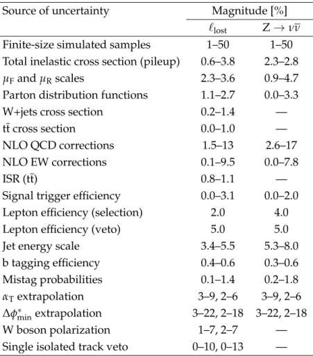
Source of uncertainty Magnitude [%]

`_lost Z→νν

Finite-size simulated samples 1–50 1–50

Total inelastic cross section (pileup) 0.6–3.8 2.3–2.8

µFand µRscales 2.3–3.6 0.9–4.7

Parton distribution functions 1.1–2.7 0.0–3.3

W+jets cross section 0.2–1.4 —

tt cross section 0.0–1.0 —

NLO QCD corrections 1.5–13 2.6–17

NLO EW corrections 0.1–9.5 0.0–7.8

ISR (tt) 0.8–1.1 —

Signal trigger efficiency 0.0–3.1 0.0–2.0

Lepton efficiency (selection) 2.0 4.0

Lepton efficiency (veto) 5.0 5.0

Jet energy scale 3.4–5.5 5.3–8.0

b tagging efficiency 0.4–0.6 0.3–0.6 Mistag probabilities 0.1–1.4 0.2–1.8 αTextrapolation 3–9, 2–6 3–9, 2–6 ∆φ∗ minextrapolation 3–22, 2–18 3–22, 2–18 W boson polarization 1–7, 2–7 —

Single isolated track veto 0–10, 0–13 —

The uncertainties from known theoretical and experimental sources are propagated through to the transfer factors to ascertain the magnitude of variations related to the following: the jet energy scale, the scale factors related to the b tagging efficiency and mistag probabilities, the efficiency to trigger on and identify, or veto, well-reconstructed isolated leptons, the PDFs [90],

µFand µR, and the modelling of jets from ISR produced in association with tt [67]. Uncertainties

of 100% in both the NLO QCD and EW corrections to the W+jets and Z+jets simulated sam-ples are also considered. A 5% uncertainty in the total inelastic cross section [91] is assumed and propagated through to the weighting procedure to account for differences between the data and simulation in the pileup distributions. Uncertainties in the signal trigger efficiency measurements are also propagated to the transfer factors. The effects of the aforementioned systematic uncertainties are summarized in Table 2, in terms of representative ranges. Each source of uncertainty is assumed to vary with a fully correlated behaviour across the full phase space of the SR and CRs.

Sources of additional uncertainties are determined from closure tests performed using control

data that aim to identify njet- or HT-dependent sources of systematic bias arising from

extrap-olations in kinematical variables covered by the transfer factors. Several sets of tests are

per-formed. The accuracy of the modelling of the efficiencies of both the αTand∆φmin∗ requirements

probed by using µ+jets events with a positively charged muon to predict those containing a negatively charged muon. Finally, the efficiency of the single isolated track veto is also probed using a sample of µ+jets events. The uncertainties are summarized in Table 2.

The simulation modelling of the nbdistributions for the Z(→νν)+jets background in the region

nb≥1 is evaluated through a binned maximum-likelihood fit to the observed nbdistributions

in data in each (njet, HT) bin of the µµ+jets CR. Additional checks are performed in µµ+jets

samples that are enriched in mistagged jets that originate from LF partons or charm quarks, or the genuine tags of b quarks from gluon splitting, through the use of loose and tight working points of the b tagging algorithm, respectively. No tests reveal evidence of significant bias in

the simulation modelling of the n_bdistribution.

Finally, the modelling of the H_Tmiss distribution in simulated events is compared to the

distri-butions observed in µ+jets and µµ+jets control data, and inspected for trends, by assuming a

linear behaviour of the ratio of observed and simulated counts as a function of H_Tmiss. Linear

fits are performed independently for each njetcategory while integrating event counts over nb

and HT, and then repeated for each HT bin while integrating event counts over njet and nb.

Systematic uncertainties are determined from any nonclosure between data and simulation as

a function of njet and are assumed to be correlated in HT (and nb), and vice versa. The

uncer-tainties can be as large as≈50% in the most sensitive Hmiss

T bins.

6

Multijet background estimation

The multijet background is estimated using the three data sidebands defined in Section 3.5.

Events in each sideband are categorized according to njet and HT. The event counts in data are

corrected to account for contamination from nonmultijet SM processes, such as vector boson and tt production, as well as the residual contributions from other SM processes. The nonmul-tijet processes are estimated from the µ+jets and µµ+jets CRs, following a procedure similar to the one described in Section 5. The corrected counts are assumed to arise solely from multijet

production. For each sideband, a transfer factor per (njet, HT) bin is obtained from simulation,

defined as the ratio of the number of multijet events that satisfies the SR requirements to the

number that satisfies the sideband requirement. Estimates of the multijet background per (njet,

HT) bin are obtained per sideband from the product of the transfer factors and the corrected

data counts.

The final estimate per (njet, HT) bin is a weighted sum of the three estimates. The multijet

back-ground is found to be small, typically at the percent level, relative to the sum of all nonmultijet

backgrounds in all (njet, nb) bins of the SR. The HTmiss/pmissT and∆φ∗minvariables that are used

to define the sidebands are determined to be only weakly correlated for multijet events, and the estimates from each sideband are assumed to be uncorrelated. Statistical uncertainties

as-sociated with the finite event counts in data and simulated event samples, as large as≈100%,

are propagated to each estimate. Uncertainties as large as≈20% in the estimates of nonmultijet

contamination are also propagated to the corrected events. Any differences between the three

estimates per (njet, HT) bin are adequately covered by systematic uncertainties of 100%, which

are assumed to be uncorrelated across (njet, HT) bins.

A model is assumed to determine the estimates as a function of nband HTmiss. The

distribu-tion of multijet events as a funcdistribu-tion of nb and HTmiss per (njet, HT) bin is assumed to be

iden-tical to the distribution expected for the nonmultijet backgrounds. This assumption is based on simulation-based studies and is a valid simplification given the magnitude of the multijet background relative to the sum of all other SM backgrounds, as well as the magnitude of the

statistical and systematic uncertainties in the estimates described above.

7

Results

A likelihood model is used to obtain the SM expectations in the SR and each CR, as well as to test for the presence of new-physics signals. The observed event count in each bin, defined

in terms of the njet, nb, HT, and HmissT variables, is modelled as a Poisson-distributed variable

around the SM expectation and a potential signal contribution (assumed to be zero in the fol-lowing discussion). The expected event counts from nonmultijet processes in the SR are related to those in the µ+jets and µµ+jets CRs via simulation-based transfer factors, as described in Sec-tion 5. The systematic uncertainties in the nonmultijet estimates, summarized in Table 2, are accommodated in the likelihood model as nuisance parameters, the measurements of which are

assumed to follow a log-normal distribution. In the case of the modelling of the H_Tmiss

distribu-tion, alternative templates are used to describe the uncertainties in the modelling and a vertical template morphing schema [29, 92] is used to interpolate between the nominal and alterna-tive templates. The multijet background estimates, determined using the method described in Section 6, are also included in the likelihood model.

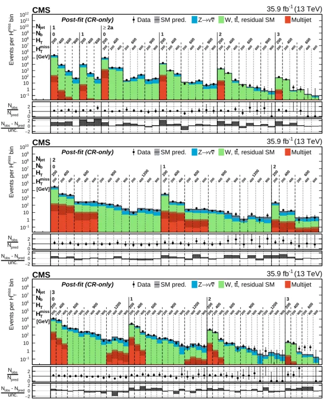
Figures 1 and 2 summarize the binned counts of signal events and the corresponding SM ex-pectations as determined from a “CR-only” fit that uses only the data counts in the µ+jets and µµ+jets control regions to constrain the model parameters related to the nonmultijet back-grounds. The uncertainties in the SM expectations reflect both statistical and systematic com-ponents. The multijet background estimates are determined independently and included in the SM expectations. The fit does not consider the event counts in the signal region.

Hypothesis testing with regards to a potential signal contribution is performed by considering a full fit to the event counts in the SR and CRs. No significant deviation is observed between the predictions and data in the SR and CRs, and the data counts appear to be adequately modelled by the SM expectations with no significant kinematical patterns.

Event counts, SM background estimates, and the associated correlation matrix are also deter-mined using the simplified 32-bin schema, which can be found in Appendix A.

8

Interpretations

The search result is used to constrain the parameter spaces of simplified SUSY models [30–32]. Interpretations are provided for nine unique model families, as summarized in Table 3. Each family of models realizes a unique production and decay mode. The model parameters are the

masses of the parent gluino (m_eg) or bottom, top, and LF (meb₁, met1, meq) squark, also collectively

labelled as mSUSY, and theχe

0

1(mχe

0

1). Two scenarios are considered for LF squarks: one with an

eightfold mass degeneracy foreqLandeqR withqe = {u, ee d,es,ec}and the other with just a single

light squark (euL). All other SUSY particles are assumed to be too heavy to be produced directly.

Gluinos are assumed to undergo prompt three-body decays via highly virtual squarks. In the case of split SUSY models (T1qqqqLL), the gluino is assumed to be long-lived with proper

decay lengths in the range 10−3 < cτ0 < 105mm. A scenario involving a metastable gluino

with cτ0=1018mm is also considered.

Under the signal+background hypothesis, and in the presence of a nonzero signal contribution, a modified frequentist approach is used to determine observed upper limits (ULs) at 95%

1 − 10 1 10 2 10 3 10 4 10 5 10 6 10 7 10 8 10 9 10 10 10 11 10 12 10 bin miss T Events per H

Data SM pred. Z→νν W, tt, residual SM Multijet

Post-fit (CR-only) (13 TeV) -1 35.9 fb CMS 1 ≥ 2a 0 1 0 1 2 3 200 400 600 900 200 400 600 200 400 600 900 200 400 600 900 200 400 600 900 200 400 600 200 200 400 200 400 600 200 900 200 200 400 200 400 600 200 900 200 200 400 200 400 600 200 900 200 200 400 200 400 600 jet N b N T H [GeV] T miss H 0 1 2 pred N obs N 2 − 0 2 unc. pred - N obs N 1 − 10 1 10 2 10 3 10 4 10 5 10 6 10 7 10 8 10 9 10 10 10 bin miss T Events per H

Data SM pred. Z→νν W, tt, residual SM Multijet

Post-fit (CR-only) (13 TeV) -1 35.9 fb CMS 2 0 1 2 200 400 600 900 1200 200 400 600 900 1200 200 400 600 200 200 400 200 400 600 200 400 600 900 200 400 600 900 200 200 400 200 400 600 200 400 600 900 200 400 600 900 200 200 400 200 400 600 jet N b N T H [GeV] T miss H 01 2 pred N obs N 2 −0 2 unc. pred - N obs N 1 − 10 1 10 2 10 3 10 4 10 5 10 6 10 7 10 8 10 9 10 bin miss T Events per H

Data SM pred. Z→νν W, tt, residual SM Multijet

Post-fit (CR-only) (13 TeV) -1 35.9 fb CMS 3 0 1 2 3 200 400 600 900 1200 200 400 600 900 1200 200 400 600 900 1200 200 400 600 200 200 400 200 400 600 200 400 600 900 200 400 600 900 200 200 400 200 400 600 200 400 600 900 200 400 600 900 200 200 400 200 400 600 200 400 600 900 200 400 600 900 200 200 400 200 400 600 jet N b N T H [GeV] T miss H 01 2 pred N obs N 2 −0 2 unc. pred - N obs N

Figure 1: Counts of signal events (solid markers) and SM expectations with associated uncer-tainties (statistical and systematic, black histograms and shaded bands) as determined from

the CR-only fit as a function of nb, HT, and HTmiss for the event categories njet = 1 and ≥2a

(upper), = 2 (middle), and= 3 (lower). The centre panel of each subfigure shows the ratios

of observed counts and the SM expectations, while the lower panel shows the significance of deviations observed in data with respect to the SM expectations expressed in terms of the total uncertainty in the SM expectations.

1 − 10 1 10 2 10 3 10 4 10 5 10 6 10 7 10 8 10 bin miss T Events per H

Data SM pred. Z→νν W, tt, residual SM Multijet

Post-fit (CR-only) (13 TeV) -1 35.9 fb CMS 4 0 1 2 3 400 600 900 1200 400 600 900 1200 400 600 900 1200 400 600 900 200 400 200 400 600 200 400 600 900 200 400 600 900 200 400 200 400 600 200 400 600 900 200 400 600 900 200 400 200 400 600 200 400 600 900 200 400 600 900 200 400 200 400 600 200 400 600 900 jet N b N T H [GeV] T miss H 01 2 pred N obs N 2 −0 2 unc. pred - N obs N 1 − 10 1 10 2 10 3 10 4 10 5 10 6 10 7 10 bin miss T Events per H

Data SM pred. Z→νν W, tt, residual SM Multijet

Post-fit (CR-only) (13 TeV) -1 35.9 fb CMS 5 0 1 2 3 4 400 600 900 1200 400 600 900 1200 400 600 900 1200 400 600 900 400 200 400 200 400 600 200 400 600 200 400 600 900 200 400 200 400 600 200 400 600 200 400 600 900 200 400 200 400 600 200 400 600 200 400 600 900 200 400 200 400 600 200 400 600 200 400 jet N b N T H [GeV] T miss H 01 2 pred N obs N 2 −0 2 unc. pred - N obs N 1 − 10 1 10 2 10 3 10 4 10 5 10 6 10 7 10 bin miss T Events per H

Data SM pred. Z→νν W, tt, residual SM Multijet

Post-fit (CR-only) (13 TeV) -1 35.9 fb CMS 6 ≥ 0 1 2 3 4 400 600 900 1200 400 600 900 1200 400 600 900 1200 400 600 900 1200 400 200 200 400 200 400 600 200 400 600 900 200 200 400 200 400 600 200 400 600 900 200 200 400 200 400 600 200 400 600 900 200 200 400 200 400 600 200 400 600 900 200 jet N b N T H [GeV] T miss H 0 1 2 pred N obs N 2 − 0 2 unc. pred - N obs N

Figure 2: Counts of signal events (solid markers) and SM expectations with associated uncer-tainties (statistical and systematic, black histograms and shaded bands) as determined from

the CR-only fit as a function of nb, HT, and H_Tmissfor the event categories njet = 4 (upper),=5

Table 3: Summary of the simplified SUSY models used to interpret the result of this search.

Model family Production and decay Additional assumptions

Production and prompt decay of squark pairs

T2bb pp→eb₁eb₁, eb₁ →bχ_e0₁ — T2tt pp→et₁et₁,et₁ →tχ_e0₁ — T2cc pp→et₁et₁,et₁ →cχe 0 1 10<met1−mχe 0 1 <80 GeV T2qq 8fold pp→_eqeq,eq→qχe 0 1 meqL = meqR,eq= {eu, ed,es,ec} T2qq 1fold pp→_eqeq,eq→qχe 0 1 meq(eq6=euL) meuL

Production and prompt decay of gluino pairs

T1bbbb pp→_egeg,eg→beb ∗ 1 →bbχe 0 1 meb₁ meg T1tttt pp→_egeg,eg→tet ∗ 1 →ttχe 0 1 met1 meg T1qqqq pp→_egeg,eg→qeq ∗ _→qq e χ0₁ m_eqmeg

Production and decay of long-lived gluino pairs

T1qqqqLL pp→_egeg,eg→qeq ∗ _→qq e χ0₁ m e qmeg, 10 −3 _<cτ 0 <105mm or metastable

mSUSY, mχ_e0₁, and cτ0(if applicable). The approach is based on the profile likelihood ratio as the

test statistic [93], the CLs criterion [94, 95], and the asymptotic formulae [96] to approximate

the distributions of the test statistic under the SM-background-only and signal+background

hypotheses. An Asimov data set [96] is used to determine the expected σUL on the allowed

cross section for a given model. Potential signal contributions to event counts in all bins of the SR and CRs are considered.

The experimental acceptance times efficiency (Aε) is evaluated independently for each model,

defined in terms of mSUSY, mχ_e0₁, and cτ0 (if applicable). The effects of several sources of

un-certainty in Aε, as well as the potential for migration of events between bins of the SR, are

considered. Correlations are taken into account where appropriate, including those relevant to signal contamination that may contribute to counts in the CRs.

The statistical uncertainty arising from the finite size of simulated samples can be as large as

≈30%. TheAε for models with a compressed mass spectrum relies on jets arising from ISR,

the modelling of which is evaluated using the technique described in Ref. [67]. The associated

uncertainty can be as large as≈30%. The corrections to the jet energy scale (JES) evaluated with

simulated events can lead to variations in event counts as large as≈25% for models yielding

high jet multiplicities. The uncertainties in the modelling of scale factors applied to simulated event samples that correct for differences in the b tagging efficiency and mistag probabilities

can be as large as≈20%.

Table 4 defines a number of benchmark models that are close to the limit of the search

sen-sitivity. All model families are represented, and the model parameters (mSUSY, mχ_e0₁, and cτ0

if applicable) are chosen to select models with large and small differences in mSUSY and mχ_e0₁,

as well as a range of cτ0values. Table 4 summarizes the aforementioned uncertainties for each

benchmark model, presented in terms of a characteristic range that is representative of the vari-ations observed across the bins of the SR. The upper bound for each range may be subject to moderate statistical fluctuations.

Additional subdominant contributions to the total uncertainty are also considered. The uncer-tainty in the integrated luminosity is determined to be 2.5% [23]. Uncertainties in the produc-tion cross secproduc-tion arising from the choice of the PDF set, and variaproduc-tions therein, as well as

vari-Table 4: A list of benchmark simplified models organized according to production and decay

modes (family), theAε, representative values for some of the dominant sources of systematic

uncertainty, and the expected and observed upper limits on the production cross section σUL

relative to the theoretical value σthcalculated at NLO+NLL accuracy. Additional uncertainties

concerning the T1qqqqLL models are not listed here and are discussed in the text.

Family (mSUSY, mχe

0

1) Aε Systematic uncertainties [%] σUL/σth(95% CL)

(cτ0) [GeV] [%] MC stat. ISR JES b tagging Exp. Obs.

T2bb (1000, 100) 40.1 14–23 1–7 4–11 1–4 0.62 0.67 (550, 450) 5.7 9–22 4–15 4–15 3–7 0.76 1.21 T2tt (1000, 50) 23.8 14–27 3–7 4–14 1–5 0.82 0.85 (450, 200) 4.2 6–19 4–12 6–15 4–9 0.56 0.73 (250, 150) 0.3 10–23 13–27 8–22 6–16 0.71 0.66 T2cc (500, 480) 20.5 6–19 4–18 5–13 1–4 0.68 1.38 T2qq 8fold (1250, 100) 42.9 12–24 2–7 5–14 1–1 0.54 0.66 (700, 600) 7.7 6–22 4–17 4–13 2–5 0.75 1.13 T2qq 1fold (700, 100) 32.9 4–22 2–7 3–10 0–5 0.60 0.88 (400, 300) 4.5 6–20 5–22 5–18 3–5 0.61 0.46 T1bbbb (1900, 100) 25.1 11–19 3–9 4–6 7–11 0.56 1.25 (1300, 1100) 14.6 11–22 2–11 3–11 2–5 0.44 1.15 T1tttt (1700, 100) 6.9 12–24 2–6 3–15 2–6 0.51 1.31 (950, 600) 0.3 15–30 5–9 12–26 2–6 0.89 1.51 T1qqqqLL (1800, 200) 27.8 8–20 3–5 3–9 0–1 1.02 1.91 (1 µm) (1000, 900) 6.7 15–21 2–10 4–14 0–1 0.68 1.26 T1qqqqLL (1800, 200) 22.9 11–20 2–5 3–9 17–59 0.43 1.00 (1 mm) (1000, 900) 5.2 17–26 2–9 4–17 10–41 0.28 0.63 T1qqqqLL (1000, 200) 11.2 16–22 2–14 4–9 0–1 0.74 1.58 (100 m) (1000, 900) 10.4 14–26 3–14 2–12 0–1 0.63 0.45

ations in µFand µRat LO are considered. Uncertainties in event migration between bins from

variations in the PDF sets are assumed to be correlated with, and adequately covered by, the

uncertainties in the modelling of ISR. Uncertainties from µFand µRvariations are determined

to be≈5%. The effect of a 5% uncertainty in the total inelastic cross section [91] is propagated

through the weighting procedure that corrects for differences between the simulated and

mea-sured pileup, resulting in event count variations of≈10%. Uncertainty in the modelling of the

efficiency to identify high-quality, isolated leptons is≈5% and is treated as anticorrelated

be-tween the SR and µ+jets and µµ+jets CRs. The uncertainty in the trigger efficiency to record

signal events is<10%.

TheAεfor the T1qqqqLL family of models depends on cτ0in addition to megand mχe

0

1. Scenarios

involving a compressed mass spectrum or gluinos with cτ0 & 10 m increase the probability

that the decay of the gluino-pair system escapes detection, and the Aε is reduced for such

models, as indicated in Table 4, because of an increased reliance on jets from ISR. Scenarios

with m_eg−mχ_e0₁ & 100 GeV and 1 . cτ0 . 10 m often lead to one or both gluinos decaying

within the calorimeter systems to yield energetic jets comprising particle candidates that have no associated charged particle track. Hence, the efficiencies for the event vetoes related to

the jet identification and fj1

h± requirements, described in Sections 2 and 3.1, can be as low as

≈90% and ≈30%, respectively, for this region of the model parameter space. Uncertainties

as large as≈10% are assumed. The efficiencies for all other scenarios are typically≈100%. Jet

identification requirements in the trigger logic lead to inefficiencies and uncertainties not larger

than 2%. Finally, models with 1 . cτ0 . 10 mm often lead to jets that are tagged by the CSV

algorithm with efficiencies as high as≈60%, which are comparable to the values obtained for

jets originating from b quarks. Uncertainties of 20–50% in the tagging efficiency are assumed to cover differences with respect to jets originating from b quarks, as indicated in Table 4. Figure 3 summarizes the excluded regions of the mass parameter space for the nine families

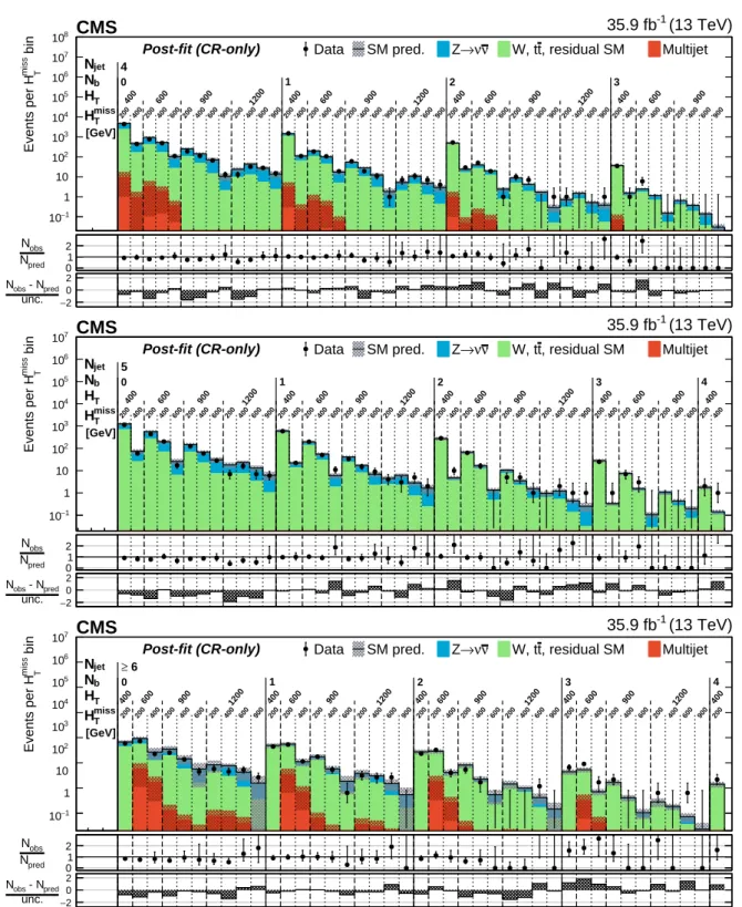
of simplified models. The regions are determined by comparing σULwith the theoretical cross

sections σthcalculated at NLO+NLL accuracy. The former value is determined as a function of

mSUSYand mχ_e0₁, while the latter has a dependence solely on mSUSY. The exclusion of models is

evaluated using observed data counts in the signal region (solid contours) and also expected counts based on an Asimov data set (dashed contours). The observed excluded regions for the T1bbbb and T1tttt families, as shown in Fig. 3 (lower), can be up to 2–3 standard deviations

weaker than the expected excluded regions when m_eg−mχ_e0₁ ≈ 350 GeV. These differences are

typically due to fluctuations in data for events that satisfy njet ≥5 and nb≥3. Figure 3 (lower)

also allows a comparison of the sensitivity to T1qqqq and T1qqqqLL models, which assume the prompt-decay and metastable gluino scenarios, respectively. The latter scenario leads to

a monojet-like final state as the gluino escapes detection, resulting in a reach in m_eg that is

independent of m

e

χ0₁.

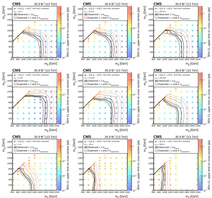
Figure 4 summarizes the evolution of the search sensitivity to the T1qqqqLL family of models as

a function of cτ0. Each subfigure presents the observed σULas a function of megand mχe

0

1for

sim-plified models that involve the production of gluino pairs. The excluded mass regions based on

the observed and expected values of σULare also shown, along with contours determined

un-der variations in theoretical and experimental uncertainties. The top row of subfigures cover

the range 1 < cτ0 < 100 µm and demonstrate coverage comparable to the T1qqqq

prompt-decay scenario. A moderate improvement in sensitivity for models with 1 . cτ0 . 10 mm

is observed because of the additional signal-to-background discrimination provided by the nb

variable. The sensitivity is reduced for models with lifetimes in the region cτ0 > 100 mm

be-cause of a lower acceptance for the jets from the gluino decay and an increased reliance on jets

from ISR. The coverage is independent of cτ0 beyond values of 10 m and comparable to the

limiting case of a metastable gluino.

A nonnegligible fraction of R-hadrons that traverse the muon chambers before decaying are identified as muons by the PF algorithm. The fraction is dependent on the R-hadron model and the choice of parameters that affect the hadronization model and matter interactions. The signal

Aεis strongly dependent on cτ0 due to the muon veto employed by this search. Under these

assumptions, the excluded mass regions shown in Fig. 4 weaken by 50–200 GeV for models

with cτ0 & 1 m, with the largest change occurring at cτ0 ≈ 10 m. The change is negligible for

models with cτ0below 1 m.

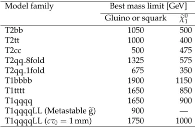
Table 5 summarizes the strongest expected and observed mass limits for each family of models. The simplified result based on the 32-bin schema, summarized in Appendix A, yields limits on

0 200 400 600 800 1000 1200 1400

[GeV]

q ~ / 1 t ~ / 1 b ~

m

0 200 400 600 800 1000 1200

[GeV]

0 1 χ∼

m

(13 TeV) -1 35.9 fb

CMS

NLO+NLL exclusion 1 m ∆ W = m 1 0 χ - m 1 t ~ m ≡ 1 m ∆ _m2 ∆ t = m 1 0 χ - m 1 t ~ m ≡ 2 m ∆ 1 0 χ∼ b → 1 b ~ , 1 b ~ 1 b ~ → pp 1 0 χ∼ (*) t → 1 t ~ , 1 t ~ 1 t ~ → pp 1 0 χ∼ c → 1 t ~ , 1 t ~ 1 t ~ → pp ) c ~ , s ~ , d~ , u ~ , R q ~ + L q ~ ( 1 0 χ∼ q → q ~ , q ~ q ~ → pp ) q ~ (one light 1 0 χ∼ q → q ~ , q ~ q ~ → pp Expected Observed

[GeV]

g ~

m

600 800 1000 1200 1400 1600 1800 2000 2200

[GeV]

0 1 χ∼

m

0 200 400 600 800 1000 1200 1400 1600 1800 2000 (13 TeV) -1 35.9 fb

CMS

NLO+NLL exclusion g ~ g ~ → pp 10 χ∼ b b → g ~ 1 0 χ∼ t t → g ~ (Prompt decay) 1 0 χ∼ q q → g ~ g ~ Metastable Expected Observed

Figure 3: Observed and expected mass exclusions at 95% CL (indicated, respectively, by solid and dashed contours) for various families of simplified models. The upper subfigure sum-marises the mass exclusions for five model families that involve the direct pair production of squarks. The first scenario considers the pair production and decay of bottom squarks (T2bb). Two scenarios involve the production and decay of top squark pairs (T2tt and T2cc). The grey shaded region denotes T2tt models that are not considered for interpretation. Two further sce-narios involve, respectively, the production and decay of light-flavour squarks, with different assumptions on the mass degeneracy of the squarks as described in the text (T2qq 8fold and T2qq 1fold). The lower subfigure summarises three scenarios that involve the production and prompt decay of gluino pairs via virtual squarks (T1bbbb, T1tttt, and T1qqqq). A final scenario involves the production of gluinos that are assumed to be metastable on the detector scale (T1qqqqLL).

[GeV] g ~ m 600 800 1000 1200 1400 1600 1800 2000 2200 [GeV]0_χ∼1 m 0 200 400 600 800 1000 1200 1400 1600 1800 3 − 10 2 − 10 1 − 10 1 (13 TeV) -1 35.9 fb CMS NLO+NLL exclusion 10 χ∼ q q → g ~ , g ~ g ~ → pp m µ = 1 0 τ c theory σ 1 ± Observed experiment σ 1 and 2 ± Expected

95% CL upper limit on cross section [pb]

[GeV] g ~ m 600 800 1000 1200 1400 1600 1800 2000 2200 [GeV]0_χ∼1 m 0 200 400 600 800 1000 1200 1400 1600 1800 3 − 10 2 − 10 1 − 10 1 (13 TeV) -1 35.9 fb CMS NLO+NLL exclusion 1 0 χ∼ q q → g ~ , g ~ g ~ → pp m µ = 10 0 τ c theory σ 1 ± Observed experiment σ 1 and 2 ± Expected

95% CL upper limit on cross section [pb]

[GeV] g ~ m 600 800 1000 1200 1400 1600 1800 2000 2200 [GeV]1 0_χ∼ m 0 200 400 600 800 1000 1200 1400 1600 1800 3 − 10 2 − 10 1 − 10 1 (13 TeV) -1 35.9 fb CMS NLO+NLL exclusion 1 0 χ∼ q q → g ~ , g ~ g ~ → pp m µ = 100 0 τ c theory σ 1 ± Observed experiment σ 1 and 2 ± Expected

95% CL upper limit on cross section [pb]

[GeV] g ~ m 600 800 1000 1200 1400 1600 1800 2000 2200 [GeV]0_χ∼1 m 0 200 400 600 800 1000 1200 1400 1600 1800 3 − 10 2 − 10 1 − 10 1 (13 TeV) -1 35.9 fb CMS NLO+NLL exclusion 10 χ∼ q q → g ~ , g ~ g ~ → pp = 1 mm 0 τ c theory σ 1 ± Observed experiment σ 1 and 2 ± Expected

95% CL upper limit on cross section [pb]

[GeV] g ~ m 600 800 1000 1200 1400 1600 1800 2000 2200 [GeV]0_χ∼1 m 0 200 400 600 800 1000 1200 1400 1600 1800 3 − 10 2 − 10 1 − 10 1 (13 TeV) -1 35.9 fb CMS NLO+NLL exclusion 1 0 χ∼ q q → g ~ , g ~ g ~ → pp = 10 mm 0 τ c theory σ 1 ± Observed experiment σ 1 and 2 ± Expected

95% CL upper limit on cross section [pb]

[GeV] g ~ m 600 800 1000 1200 1400 1600 1800 2000 2200 [GeV]1 0_χ∼ m 0 200 400 600 800 1000 1200 1400 1600 1800 3 − 10 2 − 10 1 − 10 1 (13 TeV) -1 35.9 fb CMS NLO+NLL exclusion 1 0 χ∼ q q → g ~ , g ~ g ~ → pp = 100 mm 0 τ c theory σ 1 ± Observed experiment σ 1 and 2 ± Expected

95% CL upper limit on cross section [pb]

[GeV] g ~ m 600 800 1000 1200 1400 1600 1800 2000 2200 [GeV]01 χ∼ m 0 200 400 600 800 1000 1200 1400 1600 1800 3 − 10 2 − 10 1 − 10 1 (13 TeV) -1 35.9 fb CMS NLO+NLL exclusion 10 χ∼ q q → g ~ , g ~ g ~ → pp = 1 m 0 τ c theory σ 1 ± Observed experiment σ 1 and 2 ± Expected

95% CL upper limit on cross section [pb]

[GeV] g ~ m 600 800 1000 1200 1400 1600 1800 2000 2200 [GeV]01 χ∼ m 0 200 400 600 800 1000 1200 1400 1600 1800 3 − 10 2 − 10 1 − 10 1 (13 TeV) -1 35.9 fb CMS NLO+NLL exclusion 1 0 χ∼ q q → g ~ , g ~ g ~ → pp = 10 m 0 τ c theory σ 1 ± Observed experiment σ 1 and 2 ± Expected

95% CL upper limit on cross section [pb]

[GeV] g ~ m 600 800 1000 1200 1400 1600 1800 2000 2200 [GeV]1 0 χ∼ m 0 200 400 600 800 1000 1200 1400 1600 1800 3 − 10 2 − 10 1 − 10 1 (13 TeV) -1 35.9 fb CMS NLO+NLL exclusion 1 0 χ∼ q q → g ~ , g ~ g ~ → pp = 100 m 0 τ c theory σ 1 ± Observed experiment σ 1 and 2 ± Expected

95% CL upper limit on cross section [pb]

Figure 4: Observed upper limit in cross section at 95% CL (indicated by the colour scale) as

a function of theeg and χe

0

1 masses for simplified models that assume the production of pairs

of long-lived gluinos that each decay via highly virtual light-flavour squarks to the neutralino

and SM particles (T1qqqqLL). Each subfigure represents a different gluino lifetime: cτ0 = 1

(upper left), 10 (upper centre), and 100 µm (upper right); 1 (middle left), 10 (middle centre), and 100 mm (middle right); and 1 (lower left), 10 (lower centre), and 100 m (lower right). The

thick (thin) black solid line indicates the observed excluded region assuming the nominal (±1

standard deviation in theoretical uncertainty) production cross section. The red thick dashed

(thin dashed and dotted) line indicates the median (±1 and 2 standard deviations in