Philip Morris International, Inc.
Equity Valuation
Melissa Isabel Santos FonsecaDissertation submitted in partial fulfillment of requirements for the degree of International Masters of Science in Business Administration, at the Universidade Católica Portuguesa, 4th of June 2012
Advisor: José Carlos Tudela Martins (Student 152109324)
Melissa Fonseca 1
A
BSTRACT
This dissertation is focused on the equity valuation of Philip Morris International, Inc., the leading publicly traded tobacco company. In other words, the work done on this paper aims at determining how much the company is worth given its current assets and position in the market. Such analysis is of great importance for shareholders and potential investors, since the market is not always able to reflect the assets’ true value. Underlying this challenge is an overview of the main equity valuation methodologies and theories, along with other aspects considered as essential in a valuation process. In this context, three methodologies were considered suitable. However, the conclusions were more influenced by the adjusted present value methodology. Philip Morris Int’ is found to be undervalued with 28.32% upside potential, a BUY recommendation. Finally, the methodologies used and results obtained were contrasted to those of UBS Investment Bank, in their report published on April 19th 2012. For a more detailed overview of the dissertation main findings, read the executive summary on appendix O.
Melissa Fonseca 2
A
CKNOWLEDGMENTS
Throughout the development of this dissertation many are those who contributed with relevant materials, emotional support, critical feedbacks and recommendations for improvement. To those people I would like to express my sincere gratitude and respect: To all my family for their unconditional support; particularly to my parents for always encouraging me to pursue my dreams and for helping me in every possible way; to Analissa Fonseca, my older sister, for her patience and support; to my advisor, professor José Carlos Tudela Martins, whose guidance and support helped me shape and review my dissertation; to all my colleagues with who I had the privilege to work with, and share knowledge; to Antonella Costa for the relevant materials provided and for our valuable discussions; and finally to Luis Viúla, for his encouragement and advices.
Melissa Fonseca 3
T
ABLE OF
C
ONTENTS
1. INTRODUCTION ... 9
2. LITERATURE REVIEW ... 11
2.1.DISCOUNTED CASH FLOW (DCF)VALUATION ... 12
2.1.1. Most Common DCF models ... 13
2.1.1.1. Equity Valuation ... 13
2.1.1.1.1. The Free Cash Flow to Equity (FCFE) valuation ... 13
2.1.1.1.2. Dividend Discount Model (DDM) valuation ... 14
2.1.1.2. Firm Valuation ... 15
2.1.1.2.1. The Free Cash Flow to the Firm (FCFF) valuation ... 15
2.1.1.2.2. The Adjusted Present Value (APV) valuation ... 16
2.1.1.2.3. Capital Cash Flow (CCF) valuation ... 19
2.1.2.2.4. The Economic Value Added (EVA) valuation ... 20
2.1.3. PMI - DCF valuation ... 21
2.1.4. Additional Issues regarding DCF valuation ... 22
2.1.4.1. Terminal Value ... 22
2.1.4.2. Discount rates ... 23
2.1.4.3. Cross – Border Valuation Implications ... 26
2.1.4.3.1. Country-specific risks ... 27
2.2.RELATIVE VALUATION ... 28
2.2.1. Identify comparable firms ... 28
2.2.2. Convert prices into multiples ... 30
2.2.2.1. Data ... 30
2.2.2.2. Multiples ... 31
2.2.3. Relative Valuation Limitations ... 32
2.2.4. PMI - Relative Valuation ... 33
3. PMI - EXTERNAL ANALYSIS ... 34
Melissa Fonseca 4
3.1.1. PESTEL Analysis ... 34
3.2.MICRO-ENVIRONMENT ... 42
3.2.1. Porter’s Five Forces Analysis ... 42
4. PMI - INTERNAL ANALYSIS ... 48
4.1.COMPANY OVERVIEW ... 48
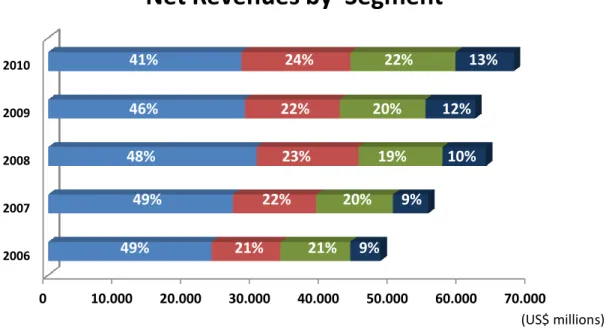
4.2.GEOGRAPHIC MIX ... 48
4.3.BRAND’S PORTFOLIO ... 51
4.4.STRATEGIC POSITION ... 52
4.5.STRATEGIES FOR GROWTH ... 52
4.6.HISTORICAL FINANCIAL PERFORMANCE ANALYSIS ... 53
4.6.1. Reorganized accounting statements ... 53
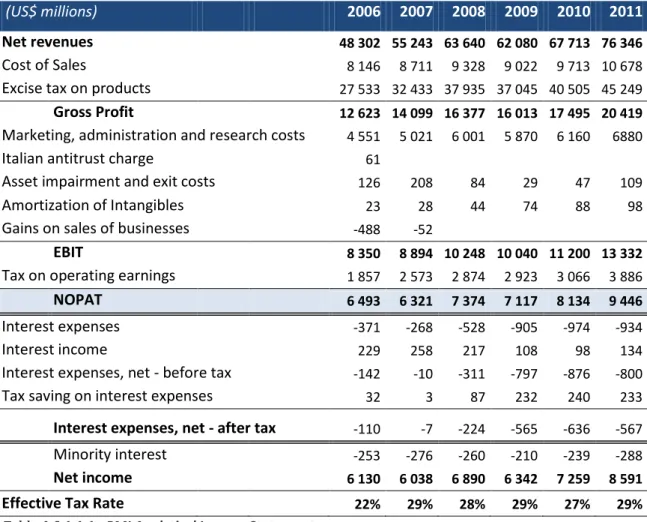
4.6.1.1. Analytical Income Statement ... 54
4.6.1.2. Analytical Balance Sheet ... 55
4.6.2. Profitability Analysis ... 56
4.6.3. Growth Analysis ... 58
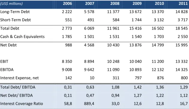
4.6.4. Financial health and capital structure ... 61
4.6.5. Stock Analysis ... 63
5. FORECAST ... 64
5.1.PMI KEY DRIVERS ... 65
5.1.1. FCFF ... 65
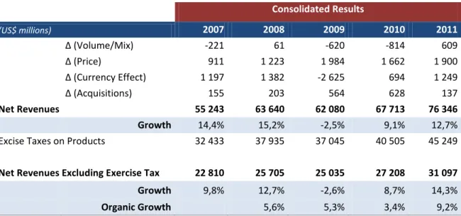
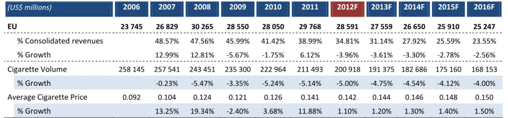
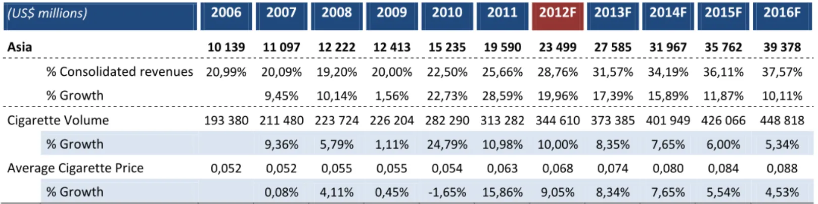
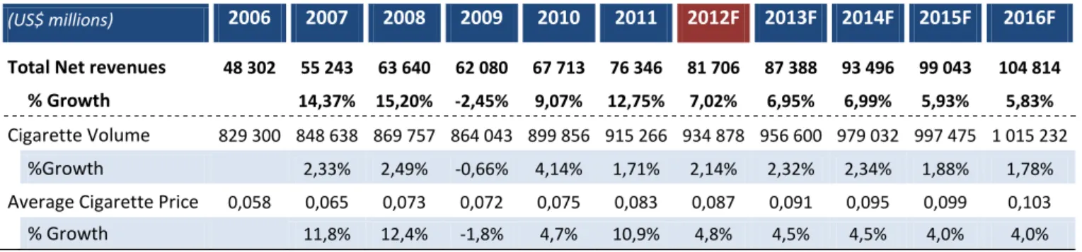
5.1.1.1. Net Revenues ... 65
5.1.1.1.1. Acquisitions ... 70
5.1.1.1.2. Currency Exchange Rate ... 70
5.1.1.2. Costs ... 71
5.1.1.2.1. Cost of Goods Sold ... 71
5.1.1.2.2. Excise Tax ... 72
5.1.1.2.3. Marketing, administration & research costs ... 73
5.1.1.2.4. Asset Impairment and Exit Costs ... 73
Melissa Fonseca 5
5.1.1.2.6. Depreciation & Amortization ... 74
5.1.1.2.7. Net Working Capital ... 75
5.1.1.2. Terminal Growth Rate ... 77
5.1.1.3. Free Cash Flow Estimation ... 78
5.1.2. Dividends ... 79
5.1.3. Financial Statements ... 79
6. PMI VALUATION ... 82
6.1.ADJUSTED PRESENT VALUE (APV)VALUATION ... 82
6.2.CAPITAL CASH FLOW (CCF)VALUATION ... 84
6.3.APV VALUATION VERSUS CCF VALUATION ... 84
6.4.RELATIVE VALUATION ... 85
6.4.1. Peer Group ... 85
6.4.2. Multiples Valuation ... 88
6.5.VERIFYING VALUATION RESULTS ... 89
6.5.1. Sensitivity analysis ... 89
6.5.2. Plausibility Analysis ... 93
6.5.3. Comparison Investment Bank ... 93
7. CONCLUSION ... 97
8. APPENDICES ... 100
APPENDIX A: DISCOUNTED CASH FLOW (DCF)MODELS ... 100
APPENDIX B:TOBACCO POLICY INSTRUMENTS ... 101
APPENDIX C:WORLDWIDE RESTRICTIONS ON TOBACCO ADVERTISING ... 102
APPENDIX D:PMI-HISTORICAL FINANCIAL STATEMENTS ... 103
APPENDIX E:PMI-HISTORICAL REVENUES RESULTS BY SEGMENTS ... 106
APPENDIX F:INFLATION ... 107
APPENDIX G:PMI-HISTORICAL DEBT STRUCTURE &INTEREST RATE ... 107
APPENDIX H:PMI-FORECASTED FINANCIAL STATEMENTS ... 108
Melissa Fonseca 6
APPENDIX J:PMI-CREDIT RATING AND RESPECTIVE DEFAULT SPREAD ... 111
APPENDIX K:PMI–APV VALUATION ... 112
APPENDIX L:PMI–CCFVALUATION ... 113
APPENDIX M:PMI–APVVALUATION VERSUS CCFVALUATION ... 114
APPENDIX N:PMI–RELATIVE VALUATION ... 114
APPENDIX O:EXECUTIVE SUMMARY ... 114
Melissa Fonseca 7
N
OTATIONS AND ABBREVIATIONS
:
a.k.a. CCF
Also known as Capital Cash Flow
CF Cash Flow D Debt DCF DDM DPS D/V
Discounted Cash Flow Dividend Discount Model Dividend Per Share
The proportion of total value claimed by debt
E Equity
EBIT Earnings Before Interest and Taxes
EBITDA Earnings Before Interest, Taxes, Depreciation and Amortizations
EPS Earnings per share
EVA E/V
Earnings Value Added
The proportion of total value claimed by equity
FCFE Free Cash Flow to the Firm
FCFF Free Cash Flow to the Equity
FF Fama and French
G Growth
GICS i.e.
Global Industry Classification Standard In other words
Melissa Fonseca 8
KA Expected Asset Return
Kd The required rate of return on debt capital
Ke NAICS
The required rate of return on equity capital North America Industry Classification Systems NOPAT
OECD PMI
Net Operating Profit After Taxes
Organization for Economic Cooperation and Development Philip Morris International, Inc.
RF Risk free
ROE Return on Equity
ROIC Return on Equity
Rp Risk Premium
SIC T
Standard Industrial Classification Taxes TV V Vu VAT Terminal Value Firm’s Value
Firm’s Unlevered Value Value Added Tax WACC
β
Weighted Average Cost of Capital Beta
Levered Beta
Melissa Fonseca 9
1.
I
NTRODUCTION
This dissertation is concerned with exploring the theoretical and practical aspects related to Equity Valuation. The main goal is to estimate the fair value of a public company, by linking theory and practice; and then compare the valuation result with the value estimated by an investment bank.
For the purpose, the company chosen was Philip Morris International, Inc. (PMI), the leading publicly traded tobacco company – listed on the New York Stock Exchange (NYSE) under the ticker of PM – and the fourth largest global consumer package goods company.
Subsequently, the overarching research question imposed in this dissertation is: What is the target price for Philip Morris International’s stock?
The research question will be answered by performing an analysis of the equity valuation methodologies as well as an in dept analysis of PMI – strategic and financial analysis, followed by forecast and valuation. Conclusively, the results will be acknowledged by conducting several checks to test the result credibility and to diminish the possibility of errors. At this point, my valuation results will be compared with the results of an investment bank, assessing and stressing the methodological discrepancies and final value differences. The investment bank chosen for the use is UBS (Union Bank of Switzerland) Investment Bank.
1.1. Dissertation structure
The remainder of the dissertation was organized in several sections. These sections represent the main steps involved in the valuation process of Philip Morris International. A brief introduction of each section is present below:
I. Section Two, the literature review, presents the different valuation approaches and methodologies available to proceed with the equity valuation of Philip
Melissa Fonseca 10 Morris International, Inc. The main goal of this section is to analyze the pros and cons of each potential valuation methodology and define the best methodologies to proceed with the valuation of the target company.
II. Section Three focuses on the external analysis of Philip Morris International. At this section, the macro- and micro-environment are analyzed with the help of the PESTE framework and Porter’s Five Forces framework, respectively. The ambition here is to identify the main challenges and opportunities present in the tobacco industry.
III. Section Four provides the internal analysis of Philip Morris International. In this section is presented the strategic analysis as well as the historical financial analysis of the company with the purpose of analyzing the company’s competitive position and ability to generate cash in the future.
IV. Section Five is devoted to forecast the key drivers of PMI future performance. Basically, the forecasts will reveal the impact that expected future changes in the macro- and micro-environment (identified in section three) will have on the current business performance (analyzed in section four).
V. Section Six presents the company’s valuation. This section describes the final steps that were taken in order to create a complete valuation and establish a price target for the company’s stock. Additionally, the section also includes several checks to test the logic of the valuation results: sensitivity analysis and a comparison with the UBS investment bank results.
VI. Section Seven is devoted to the presentation of my final remarks and potential limitation of the research subject.
Melissa Fonseca 11
2. LITERATURE REVIEW
This section aims to provide the theoretical background required to proceed with the valuation of Philip Morris International, Inc. (PMI). Nevertheless, as you continue reading you will realize that valuation is far from straightforward. There are multiple paths/techniques available to lead to “the correct” asset value and no specific rule to support the choice of the best suited technique to go along with the valuation1. As a result, the important task is to extract from the pool of techniques the one that best fits the valuation of PMI, in other words, the technique which present the most direct way, with less probability of mistakes throughout the estimation process and for which it is available the most accurate data.
In a more comprehensive way, Damodaran (2006) identified four ways of valuing a firm. Nonetheless, as a starting point, the analysis has been narrowed to two of these approaches only: Discounted Cash Flow valuation which discounts the future cash flows to get the present value of a firm or equity, and Relative valuation which values a firm regarding the value of comparable firms. The other two approaches that were then disregarded of the purpose of the report were: the Asset-based Valuation which separately computes the current value of all assets of the firm and the Contingency Claim Valuation that uses the option pricing model to value opportunities. The reasons for doing so were that first, regarding the Contingency Claim models, PMI’s business does not present the characteristics for the application of option pricing models; and second, the reason for not engaging into further analysis of the asset-base valuation approach was because due to its accounting nature, it revealed suitable only for firms with mostly fixed assets, little or no growth opportunities and no potential for excess returns, which is not the case of PMI (Damodaran 2006).
1‘All Roads lead to Rome’ 2
Damadoran, A. (1998) ‘Value Creation and Enhancement: Back to the Future’, Stern School of Business, 1-72.
3
According to Magni and Vélez Pareja, potential dividends are the cash available for distribution that can be distributed or can be retained by the firm, i.e., FCFE.
4
In ‘Corporate Uses of Beta’ by Rosenberg and Rudd: According to CAPM, WACC is the overall cost of debt and equity expressed like equation [6].
Melissa Fonseca 12
2.1. DISCOUNTED CASH FLOW (DCF) VALUATION
Making the bridge between the present and the future value of a firm, discounted cash flow models use expectations regarding cash flows generation in the future to estimate the present value of a firm. That is, considering a firm as a group of assets, the DCF models compute the value of a firm based on one of the basic principles in finance which states that “the value of any asset can be viewed as the present value of the expected cash flows on that asset”2. On the words of Luerhman (1997): “discounted cash flow analysis regards business as a series of risky cash flows stretching into the future”.
Mathematically, the approach is expressed like this:
i
n n
Equation [1] exhibits the cash flows that the company is expected to generate over its life discounted at a rate that reflects the uncertainty. This equation is applicable to all DCF methodologies, besides the use of different cash flows and discount rates – in which the discount rate increases with the riskiness of the cash flows being discounted. (Illustrated in appendix A)
In reality, the employment of this approach is far more complex than it might appear at first sight. Bearing in mind that a public firm has an infinite life, in order to estimate the value of a firm through DCF analysis, we need to measure not only the cash flows of the investments that have already been made, but also estimate the value from future growth. Consequently, to proceed with any discounted cash flow analysis, we need to estimate cash flows, future growth and the appropriate discount rate.
2
Damadoran, A. (1998) ‘Value Creation and Enhancement: Back to the Future’, Stern School of Business, 1-72.
Melissa Fonseca 13
2.1.1. MOST COMMON DCF MODELS
There is a wide range of DCF models, which can differ according to couple dimensions. Firstly, DCF valuation can be characterized as an “Equity valuation” if the methodology in place values only the equity stake; or as a “Firm valuation” if it values the company as a whole. Secondly, we can also distinguish between “Total Cash Flow” and “Excess Cash” models. “Total Cash Flow” models estimate the present value of all cash flows generated by an asset whereas “Excess Cash” models estimate only the present value of excess cash flows.
The following table exhibits the most common DCF models that will be studied and considered for PMI´s valuation.
Equity Valuation Firm Valuation
Total Cash Flow FCFE ; DDM FCFF ; APV ; CCF
Excess Cash Flow Dynamic ROE EVA
Table A: Most Common DCF methodologies
2.1.1.1.EQUITY VALUATION
2.1.1.1.1. THE FREE CASH FLOW TO EQUITY (FCFE) VALUATION
Equation [2] shows that common equity can be directly estimated by discounting free cash flow to equity (FCFE) at the cost of equity (Ke). In doing so, you will be valuating just the equity stake, which is the cash flow available for equity investors. It is written as: E i n E E n [2]
Melissa Fonseca 14 2.1.1.1.2. DIVIDEND DISCOUNT MODEL (DDM) VALUATION
A special case for valuing the cash flow available for shareholders is the Dividend Discount Model (DDM).This approach focus on wealth distribution since it defines the intrinsic value of a firm as the present value of expected future dividends (Div) discounted at the cost of equity (ke) - equation [3]. It is a very intuitive approach given that dividends are the only tangible cash flow to investors (Damodaran 2006). Arguments in favor of this approach over the FCFE method have been presented by Magni and Vélez-Pareja (2009), who claimed that “potential dividends3 that are not distributed, reinvested or retained, should be ignored in firm valuation, because only distributed cash flows add value to shareholders”. The two authors also alleged that shareholders are not interest in investing in positive-NPV projects if they will never receive any cash. Thus, if a firm pays out no dividends over the life of the enterprise, the equity’s value should be zero.
E i
n E E n
Gordon made some simplifying assumptions regarding the dividends and the discount rate present in equation [3] to get a simple valuation procedure, which is known as Gordon growth model (GGM). It is one of the most widely known DDM model and it assumes that the dividends grow at a constant rate forever while the cost of equity remains constant.
t E
Even though according to some authors DDM, GGM inclusive, is the theoretical correct approach for valuing common stocks, it has two well-known limitations related to its
3
According to Magni and Vélez Pareja, potential dividends are the cash available for distribution that can be distributed or can be retained by the firm, i.e., FCFE.
[3]
Melissa Fonseca 15 application: (1) the first problem is that due to the non-existent relationship between value creation and value distribution, it is very difficult to forecast the dividends required for the DDM analysis (Miller & Modigliani 1961), and (2) the model ignores internal growth through retained earnings.
2.1.1.2.FIRM VALUATION
2.1.1.2.1. THE FREE CASH FLOW TO THE FIRM (FCFF) VALUATION
Alternatively to equity valuation is the valuation of the firm as a whole (debt plus equity). The estimation of a firm’s value is then made by discounting expected free cash flow to the firm (FCFF), i.e. the cash flows after covering all reinvestment needs and taxes, but prior to interest and principal payments, at the weighted average cost of capital (WACC). FCFF method also known as WACC model is one of the most used approaches and is expressed as follow:
i
n n
Unlike FCFE, FCFF includes both debt and equity which implies that we must account for the side effects of debt financing (interest tax shields and bankruptcy costs) in the valuation. In this approach, all the financing side effects are included in the valuation by reducing the discount rate (WACC), rather than by including them in the cash flow to investor (Shrieves and Wachowicz 2001). Then, the correct discount rate for FCFF is the WACC which is lower than the cost of equity4.
E D
According to Miles and Ezzell (1980) the weighted average cost of capital is based on the underlying assumption that the company being valued maintains the same capital structure proportions throughout time. This has been presented as being the main
4
In ‘Corporate Uses of Beta’ by Rosenberg and Rudd: According to CAPM, WACC is the overall cost of debt and equity expressed like equation [6].
[6] [5]
Melissa Fonseca 16 weakness of the WACC model, since it makes the model suitable only for firms with the simplest and most static of capital structure (Luerhman 1997). That is, considering more complex capital structures, the likelihood of mistakes significantly increases due to the periodically adjustments that the approach requires.
2.1.1.2.2. THE ADJUSTED PRESENT VALUE (APV) VALUATION
The adjusted present value model also known as “APV model” or “valuation in parts”, was first introduced by Steward Myers in 1974 while trying to understand the interaction between corporate finance and investment decisions. The method follows the Modigliani and Miller’s teachings which suggest that a company’s choice of capital structure only affects its enterprise value due to market imperfections such as: taxes and bankruptcy costs.
Most specifically, the method relies on the “principle of value additivity”5. That is, the method separately analysis the cash flows coming from the business operations and the side effects associated with its financing program; and then adds them at the end to get the “real” enterprise value of the company. Embedded in the definition above, APV is based on three basic steps, which make it a more complex model than the ones presented so far.
The first step consists on estimating the operational side of the company regardless of the company’s capital structure; i.e. the value of operations as if the company was all-equity financed (VU). The procedure is similar to the FCFF method but the discount rate
is the unlevered cost of equity (Ku) instead of WACC. (Equation 7)
i n n
5 uehrman ( 997), page 35 of ‘What’s it worth?’.
Melissa Fonseca 17 In reality, the complexity of the APV model lies in the second step in which we need to consider the company’s capital structure and estimate its financing side effects. Among several components that could be considered, the most relevant ones are the interest tax shields and the bankruptcy costs (direct and indirect costs). Both components are an increasing function of a company’s financial leverage; wherein interest tax shields adds value to the valuation and the bankruptcy costs destroys value.
In what concerns the value of tax shields, the most controversial thing is the rate at which the interest tax shields should be discounted. Fernández (2008) compared nine different theories and concluded that the divergences among the theories emerge from the calculation of the present value of the interest tax shields. According to Myers (1974), the present value of interest tax shields is obtained by discounting the interest tax shields at the required return to debt (Kd). The implicit assumption is that the interest tax shields derived from the use of debt are just as risky as the debt itself. In opposition, some authors6 suggest the use of the cost of equity as the discount rate. In 1997, Luehrman agreed with Steward Myers and considered the cost of debt as the best discount rate although in some cases an upward adjustment might be essential. The upward adjustment is appropriate for companies facing extreme conditions where tax shields are riskier than interest payments. Consequently, in those cases, the appropriate discount rate is the cost of debt plus the company probability of default (Damodaran 2002). Additionally, in cases where the company’s debt grows with operations, Ruback (2002) stated that the risk of tax shields equals the risk of operating assets7. D D i D D D n 6
Milles and Ezzel (1980) and Harris and Pringle (1985)
7 Capital Cash- Flow Model
Melissa Fonseca 18 A firms’ debt level has also implications regarding its expected bankruptcy costs. The present value of expected bankruptcy costs (BC) is expressed as equation [9] and it is the most significant estimation problem imposed by the APV valuation.
Where: i i D i
The estimation problem imposed by equation [9] is that none of its inputs are easily quantified or directly estimated. Then, although the literature provides us alternative ways to estimate them, the results might come with some level of error. Regarding the probability of default [P(D)], the most common approach is to estimate a bond rating and use the default probability associated with that rating. The present value of bankruptcy cost is the present value of the average loss in a firm’s value in case of bankruptcy. It can be computed by multiplying the estimated percentage loss (%BC) by the firm’s unlevered value in each year. This percentage loss can be estimated from studies that have looked at the scale of this cost in actual bankruptcies. (Damodaran 2002)
Finally, the third step is the sum of the different components. The value of the operating assets will be the firm’s unlevered value (Vu) plus the present value of tax shields (PVTS) minus the present value of expected bankruptcy costs (PVEBC). The PVTS must be multiplied by the probability of no default [1-P(D)], because this value only occurs when the company is operating. Then, to get a company enterprise value, we add to the value of operating assets, the value of excess cash and the value of other nonoperating assets (Koller et al. 2005).
Melissa Fonseca 19
Besides the complexity inherent in the APV model, many academics argue that it is worth the effort. Luehrman (1997) strongly advices the use of the APV method, first because due to the “principle of value additivity”, it allows the use of different rates to discount different cash flows, given their riskiness; second, he stresses that due to its exceptionally transparency, managers can analyze not only how much an asset is worth but also its origin.
2.1.1.2.3. CAPITAL CASH FLOW (CCF) VALUATION
Recently proposed by Ruback (2002), Capital Cash Flow (CCF) also defined as Compressed APV, presents its simplicity as its main advantage over the other approaches for firm valuation.
When compared to the FCFF method (present in section 2.1.2.2.1), the two models differ in the way they incorporate the side effects of debt financing. Contrasting FCFF method, CCF adds the interest tax shields in the cash flows rather than deducting them in the discount rate. Therefore, since the capital cash flow stands for “all cash available to capital suppliers, including the interest tax shields” (Ruback 2002), it must be discounted at a before- tax rate. Then, the appropriate discount rate for those cash flows corresponds to the riskiness of the assets (KA).
A i
n A A n
Directly comparing CCF with FCFF, we could say that this approach overcame the criticisms made to the use of WACC in section 2.1.1.2.1. That is, since CCF incorporates the interest tax shields in the cash flows, this model is appealing for valuing firms which capital structure substantially changes over time, because unlike FCFF the
Melissa Fonseca 20 discount rate in this model is independent of the capital structure not requiring periodically re-estimations.
The argument of simplicity was also applied in favor of CCF when compared to APV. As stated previously, Ruback (2002) believes that interest tax shields share the same risk as operating assets. For this reason, CCF discounts the interest tax shields at the risk of assets (KA), while APV discounts them at a less risky rate - the risk of debt (Kd). As a result, Ruback asserted that the APV model needs a tax adjustment when unlevering an equity beta to calculate an asset beta, turning APV into a more complex model than CCF (Ruback 2002).
2.1.2.2.4. THE ECONOMIC VALUE ADDED (EVA) VALUATION
Pioneered by Stern Stewart, this approach has been gaining its space on the financial community as a new form of performance measurement. Different from the valuation approaches discussed so far, EVA is an excess cash flow model, that is, it proposes to measure only the cash that is earned in excess of the total cost of capital (Chen and Dodd 2001). Thus, the underlying concept in this approach is that a healthy firm should earn at least its cost of capital.
The procedure to measure EVA is:
Then, the connection between EVA and the firm’s value is made through the following equation8: Assets in Place t, Assets in Place t t, Future Projects t 8
Damodaran, A. (2006) ‘Valuation Approaches and Metrics: A Survey of the Theory and Evidence’, page 38/77.
[12]
Melissa Fonseca 21 The promoted idea of investing only in projects with positive EVA, i.e., investing in projects in which the return exceeds the capital invested, is an attractive concept for investors (Chen and Dodd 2001). However, Brewer et al. (1999) pointed out some limitations for the use of EVA, among which are highlighted the following: (1) its short term orientation put emphasis on immediate results and jeopardizes investments in innovative projects, (2) its accounting nature can be subject of manipulation and (3) it is unable to adjust for size differences across plants/divisions. Hence, the authors affirm that EVA should be seen as “a piece of the performance valuation puzzle” and suggests the use of the balanced scorecard system9 developed by Kaplan and Norton (1992), where EVA would be linked to other financial and non-financial performance measures.
2.1.3. PMI - DCF VALUATION
When deciding upon the most suitable DCF technique to value PMI’s performance, a significant weight was attributed to the company expected debt to asset value proportion for the next years. PMI has been carrying significant debt in its balance sheets, showing a tendency to increase the value of debt relative to its asset value. Thus, in the absence of disclosed information regarding the company’s capital structure for the upcoming years, it is possible that PMI will keep changing its capital structure in order to better suit its financing needs. Therefore, in the presence of a leverage growing firm with an eventual unstable capital structure for the next years, the adjusted present value (APV) approach appears as the most reliable path for me to follow in order to reach an “accurate” value for PMI’s performance.
As claimed by Miles and Ezzell (1980), the FCFF (WACC) model presupposes that the company maintains the same capital structure all over the years through a periodic or continuous rebalance of its capital structure. Thus, by opting for the APV approach, I am avoiding the eventual errors that might appear with the required adjustments to
9
“Balance scorecard is a set of measures that gives top managers a fast but comprehensive view of the business… It allows managers to see business from four important perspectives: financial perspective, customer perspective, internal business perspective and innovation and learning perspective” (Kaplan and Norton 1992 p. 174)
Melissa Fonseca 22 the WACC, while also having a more detailed valuation where I can analyze the origin of PMI’s value.
Additionally, a Capital Cash Flow (CCF) valuation will also be performed to ensure the quality of the valuation. By comparing the outcomes of APV valuation and CCF valuation, I will be able to check if, in practice, under the same set of assumptions different methodologies generate similar outputs.
2.1.4. ADDITIONAL ISSUES REGARDING DCF VALUATION
2.1.4.1.TERMINAL VALUE
A very important issue that we have to deal with in all DCF analysis is the infinite life of public firms. As it is perceptible, DCF’s formulas have two different elements in the numerator: the specific cash flow forecasts and the terminal value. The reason beyond such differentiation is that since we cannot accurately estimate cash flows forever, users of DCF methods assume that beyond several years of cash flow forecasts (terminal year), cash flows will grow at a constant rate forever (terminal value). The computation and use of the terminal value is then the most simple and consistent way to deal with the uncertainty surrounding the future value of a firm, which represent a significant element intrinsic in the calculation of any DCF methodologies (Holt at al. 1999). It is expressed through a perpetuity formula.
t
t
Equation [14] portrays the estimation of the terminal value where the discount rate and the growth rate in the model are sustainable forever. At this point, the challenge is to define when the company will reach steady state and the cash flows’ terminal growth rate (TGR). Regarding the TGR it is important to emphasize that, in the long-term, no company can growth faster than the economy in which it operates. Therefore, the most common approach is to compute TGR as a steady rate equal to the projected nominal or real growth of GDP of the economy in which it operates. The choice for nominal or real growth of GDP depends on the nature of the cash flows
Melissa Fonseca 23 forecast. Additionally, Koller et al. (2005) claims that in the terminal year, capital expenditures equals depreciation and amortizations.
2.1.4.2.DISCOUNT RATES
It was previously presented the most common approaches for cash-flow valuation. According to the financial theory, each cash flow stream must be discounted at a proper discount rate that reflects their riskiness. Hence, at this stage, I will discuss the issues related to the estimation of the discount rates required in PMI valuation: cost of unlevered/levered equity and the cost of debt.
The cost of debt (KD) measures the cost of borrowing from external entities. For
companies with high credit ratings (debt rated at BBB or better) a suitable proxy is the yield to maturity of the company’s long-term debt. A straightforward way to estimate the yield to maturity is by converting the company’s bond rating into a yield spread which will be added to the risk free rate. Then, the cost of debt for high rated companies such as PMI, is easy to compute and it consists on adding to the U.S. 10-year government bond (risk free rate) the 10-10-year yield to maturity (yield spread). Regarding the cost of equity, the correct approach for its calculation seems to be more controversial. Among several risk and return models to compute the cost of equity, the most accepted, although not perfect, is the Capital Asset Pricing Model (CAPM). Developed by Sharpe (1964) and Lintner (1965), this model works under the assumption that return is positively correlated with risk and that investors are exposed only to systematic risks due to their well-diversified portfolios. The model presents the cost of equity as risk free rate plus a risk-premium that depends on the company systematic risk (measured by beta - β). Concerning the capital structure of the company we can either use the unlevered beta (βU) to obtain the cost of unlevered
equity (KU); or the levered beta ( ) to compute the cost of levered equity (KE). The
cost of unlevered equity (equation [15]) must be lower than the cost of levered equity (equation [16]) because as the debt ratio increases, increases the unpredictability of shareholders return in case of financial distress ( > U).
Melissa Fonseca 24
U F U M F E F M F
The inputs of the CAPM formulas above (risk-free rate, risk-premium and beta) are analyzed below.
Risk Free Rate (RF)
The risk free rate is the expected return on an asset with no default risk, i.e., the return on an asset that displays no uncertainty regarding its future returns (government securities). According to Damodaran (2000) in order to match the actual return to the expected return, there should be no reinvestment risk (zero coupon rates). In practice, however, for the sake of simplicity the last condition is normally ignored.
Then, the best estimation for risk free rate is by considering the rate of a government security which respects “the consistency principle”. That is, the maturity, the currency and whether the chosen government security should be real or nominal depend on the cash flows being measured. Therefore, for the valuation of PMI, since results are in nominal US dollar terms, the most accurate risk free rate estimation will be the nominal US 10-year Treasury bond rate. Longer-maturity securities could be chosen, however, according to Koller, et al. (2005 p. 312) the 10-year government bond is the rate that best matches the whole cash flow stream being measured because bonds with longer maturities might match cash flow stream better, but their illiquidity can cause stale prices and yield premiums.
Equity Risk Premium (RM-RF)
The equity risk premium reflects the difference between the market’s expected return and the risk free rate. Basically, it is the price attributed to the perceptive risk of the economy and is determined by macro-economic volatility, behavioral components and investors risk aversion.
According to Damodaran (2012) there are three basic approaches for the estimation of equity risk premium: the survey approach that consists on estimating the equity risk premium by directly asking investors the amount required as expected returns; the
Melissa Fonseca 25 historical return approach that as the name suggests relies on the past performance of the equity market; and finally the implied approach where it is used expectations regarding market future performance to estimate the current equity risk premiums. The most common approach to estimate the equity risk premium is by inferring it from past market returns relative to riskless investments (Goetzmann and Ibbotson 2005). However, Fernandez (2003) claimed that in valuation the required equity risk premium is an expectation and therefore has little to do with history. Following the same line of thinking, Damodaran (2012) affirmed that for equity research purposes is more appropriate to use the current implied equity risk premium, in order to make the valuation neutral. Additionally, when the equity risk premium is used to compute a cost of capital, a more prudent approach would be to build a long-term average of implied premium.
Beta (β)
The beta coefficient measures a stock’s systematic risk, in other words, it measures the stock exposure to the risks that can not be diversified away. It reflects the tendency of a stock’s return to respond to fluctuations in the broad market; the higher the coefficient the more it intensifies market swings (Rosenberg and Rudd 1998).
Then, a stock’s systematic risk, as measured by beta, can be closely estimated from a regression relationship based on a stock’s historical return and market returns (Rosenberg and Rudd 1998). The time frame of the regression should be at least three years and the returns monthly (Damodaran 2002). However, there are some problems with this approach: (1) the market index composition may be biased; (2) the regression may present a standard error so large that the estimation turns out to be worthless and (3) finally, the beta may change over time as firms changes. Consequently, Copeland et al. (2000) advises to use published estimates of beta for public companies, which was done in PMI valuation, jointly with some personal calculations.
Melissa Fonseca 26 The relationship between the unlevered beta and levered beta is mathematically expressed like this:
U
As mentioned before, the unlevered beta is always smaller than the levered beta due to the debt priority over equity in being paid in case of financial distress.
2.1.4.3.CROSS –BORDER VALUATION IMPLICATIONS
In today’s increasingly global marketplace, managing and consequently valuing cross-border investments have been assuming a prominent place in equity valuation. The relaxation of capital controls and the liberalization of the stock market have presented companies with new challenges, new opportunities and the world as competitors. As a result, in order to remain competitor, companies are carefully pondering cross-border investments, such as whether or not to seek for markets overseas, explore the growth potential of emerging markets or seek for cheaper resources abroad.
Together with the worldwide diversification benefits also come additional costs, risks and some specific issues that should be considered in the valuation of an international company, such as PMI. Cross-border investments involves dealing with different currencies, different corporate tax rates, different requirements regarding the timing of tax payments across countries, additional risks, among others specific issues (Kester and Morley 1997). Then, although the valuation techniques are the same everywhere, the new factor here is how to deal with these issues and incorporate them in the valuation.
At this point, the choice of which currency to proceed with the valuation as well as the other issues mentioned above should be tailored to suit the specific valuation in case and should not influence the end result. However, the following topic addresses one main point in cross-border valuation that is a source of disagreement among academics, and if not carefully analyzed might introduce errors into the analysis.
Melissa Fonseca 27 2.1.4.3.1. COUNTRY-SPECIFIC RISKS
When diversifying internationally, mostly when exploring the growth potential of emerging markets, firms are exposed to country-specific risks, such as: high levels of inflation, political changes, exchange rate fluctuations, capital controls and macroeconomic volatility (James and Koller 2005). There are two ways of reflecting those risk into the FCFF method: we can either add a risk premium to the discount rate or reflect them in the cash flows through a scenario analysis, that is, estimate an expected cost of expropriation for each year and use them to adjust the expected future cash flows of a project (Kester and Moley 1997).
Recently, many academics have been pointing out some reasons for reflecting the country-level risks into the cash flows rather than adding a risk premium to the discount rate10. First, since discount rates should reflect only non-diversifiable risks, adding a country risk premium is inappropriate in global investment portfolios because in those cases the country risks can be diversified away due to the low correlation between the risks of developed and emerging markets. In addition, the correct size of the premium is very difficult to estimate and may result in the introduction of errors into the analysis. Lastly, this approach gives managers little insight about when and how the specific risks affect a company’s value.
Then, according to the literature, the incorporation of a risk premium in the discount rate to reflect country-specific risks should be considered only for short-term valuations; the premium must be carefully defined based on realistic assumptions; and the results must be carefully interpreted considering the uncertainty surrounding the premium value (Goedhart and Haden 2003).
Fortunately, considering that PMI is a widely international firm with business in both developed and emerging markets, country-specific risks do not raise problems to the valuation as they are diversified away.
Melissa Fonseca 28
2.2. RELATIVE VALUATION
In relative valuation, the estimations of asset values are obtained by examining market prices of similar assets. There are three essential steps in relative valuation: (1) identify comparable firms, (2) convert prices into multiples of earnings, book values, or sales, and (3) compare the multiple of the firm subject of valuation with the multiples of the comparable set.
The worldwide use of relative valuation approach is justifiable by its simplicity. Throughout time, analysts have been using multiples to complement or substitute more complex approaches. As stated by Liu et al. (2011), while multiples avoid the complexity inherent in the DCF models, such as: explicit forecasts, selection of appropriate discount rates and terminal value calculation; they are based on the same principle underlying the more complex approaches: “value is an increasing function of future payoffs and a decreasing function of risk”.
2.2.1. IDENTIFY COMPARABLE FIRMS
The identification of the appropriate peers is a vital and conditional step for the excellence of the valuation using multiples. Challenges here arise when deciding upon the most suitable and reliable criteria to use in order to recognize truly comparable firms.
Several analysts consider as comparable firms the ones operating in the same sector/industry, because they believe that once in the same industry, firms do share similar growth, risk and cash flow profiles, which improve the quality of the comparison. However, arguments were presented by many academics, first questioning the quality of the industry classification and second, pointing out that even within an industry it is possible to find huge differences between companies.
Addressing the first issue, we should realize that when considering firms from the same industry as comparable firms, we must first question the quality of the companies’ industry assignment. Among the industry classification systems in practice
Melissa Fonseca 29 huge differences are exhibited in terms of methodology, structure, allocation of firms and concordance (Bhojraj et al. 2003). Then, a careful look on the industry classification systems available is important if you want to use the industry as a criterion to identify comparable firms.
The industry classification systems which are normally used are: Standard Industrial Classification (SIC) codes, Global Industry Classification System (GICS), Fama-French (FF) and North America Industry Classification Systems (NAICS).
Standard Industrial Classification (SIC) codes have proved to be useless. Clarke (1989) and Chan et al. (2007) agree that since SIC allocate firms to an industry considering their end-products or production process, it has been losing its value with the business reformulation, changes in the variety of products, growing importance of services and the shifts in technology.
On the other hand, Bhojraj et al. (2003) and Chan et al. (2007) claimed that GICS leads to lower errors than other systems. The Global Industry Classification Standards (GICS), jointly developed by Morgan Stanley International and Standard & Poors, allocates firms to an industry by considering its revenue’s origin, its earnings, and the market perception through an eight-digit classification. The main reason for the superior performance of GICS pointed by these authors is that unlike SIC and NAICS, GICS industry groupings are established to meet the needs of investment professionals and are not primarily shaped by firms’ production technology.
Although not totally denying the advantages of an industry based peer group, many have argued that being in the same sector or industry is not a sufficient argument (Damodaran 2006 p. 65 , Goedhart et al. 2005 p. 2).
Goedhart et al. (2005) state that investors have different expectations regarding each company’s ability to create value going forward; the peer group should be chosen taking into consideration investors’ expectations for growth and ROIC, instead of just focusing on the industry they are in. On the other hand, Damodaran (2006) argues that
Melissa Fonseca 30 regardless of the industry, a comparable firm is one with cash flows, growth potential, and risk similar to the firm being valued.
Statistical techniques such as cluster analyses are also an alternative way of defining comparable firms, even though Chan et al. (2007) argues that stock grouping based on industry exhibits high homogeneity than the ones formed from statistical cluster analysis.
In my understanding, all criteria presented above have at a certain point its pros and cons. For Philip Morris International Inc. peer group I will opt to combine the different criteria and get the best of each one. I will start by using GICS to narrow my initial list of potential peers and then use the help of financial and non-financial figures to find PMI’s comparable firms.
2.2.2. CONVERT PRICES INTO MULTIPLES
The second step in relative valuation is to generate standardized prices that are comparable, usually by converting prices into multiples. In this stage, it is important to consider two things: (1) the data that will be used to compute the multiples, and (2) the multiple/s that is/are more appropriate and accurate for the analysis of the target company.
2.2.2.1.DATA
In the numerator of a multiple, you should always have the latest available market price of the figure used. However, according to the data used for the value driver in the denominator, multiples can be classified as forward or historical multiples. Therefore, in relative valuation, the choice of which data to use is as important as the other steps, stressing that any analysis is only as accurate as the data it relies on. After comparing the characteristics and performance of historical and forward multiples, many authors presented arguments in favor of the second one. Authors11
11
E.g., Damodaran (2002); Goedhart, Koller & Wessels(2005); Liu, Nissim & Thomas(2002) or Lie &Lie, among others.
Melissa Fonseca 31 recognize that forward looking multiples promote greater accuracy in pricing than historical based multiples. Additionally, Liu, Nissim & Thomas (2002), highlighted that not only forward earnings are better as its performance improves if the forecast horizon increases and its earnings forecasted over different horizons are aggregated. As last resort, if no reliable forecasts are available, Goedhard et al. (2005), advice the use of the latest historical data possible- trailing data.
2.2.2.2.MULTIPLES
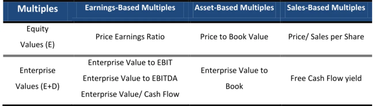
Multiples based models can be thought as special cases of the DCF models we have already discussed, in which we consider only the terminal value (represents on average 90% of the market value) and make no specific assumptions.12 Accordingly, such as in DCF models, multiples can be separated into equity13 and enterprise values14. Equity-based multiples can thus be interpreted as a simplification of more complex equity-based models (e.g. dividend discount model), whereas the enterprise-equity-based multiples stand as a simplification of more complex enterprise value based approaches (e.g. Free Cash Flow to Firm).
Another possible classification for multiples is according to the common variable used to standardize prices, such as earnings, asset or sales.
Multiples Earnings-Based Multiples Asset-Based Multiples Sales-Based Multiples
Equity
Values (E) Price Earnings Ratio Price to Book Value Price/ Sales per Share
Enterprise Values (E+D)
Enterprise Value to EBIT Enterprise Value to EBITDA Enterprise Value/ Cash Flow
Enterprise Value to
Book Free Cash Flow yield
Table 2.2.2.2.1.: Multiples
12 Young, M., Sullivan, P., Nokhasteh, A., and Holt, W. (1999) 13
Equity Value is the price multiplied by the number of shares outstanding, which estimate the value of a firm to shareholders;
14
Enterprise Value is the value of equity plus the value of debt, which deliver the value of a firm to the whole enterprise.
Melissa Fonseca 32 Table 2.2.2.2.1. exhibits the most popular multiples. However, the preference for one approach over the others depends on the company that is being subject to valuation. Lie & Lie (2002) examined the valuation accuracy of the 10 most common multiples for all active companies within the Compustat North America data base, and one of their conclusions was that the accuracy level of each approach depends on the characteristics of the company being valued, such as size, risk, profitability, level of intangible assets and being or not a financial firm.
In a more general context, Lie & Lie (2002) reached the conclusion that asset-based multiples provide the most accurate estimates whereas the sales multiples provide the least accurate estimates. The earnings based multiples provide accuracy in-between for average companies; however being as well as or better than the other multiples for companies with high earnings. In the same line of studies, Liu, Nissim and Thomas found that earnings forecasts are better summary measures of value than all other measures.
In addition, regarding earnings-based multiples, Lie & Lie (2002) suggested the use of EBITDA instead of EBIT and net income. Consistent with the results of Lie & Lie (2002), Goedhart et al. (2005), also recommend the use of enterprise value to EBITDA over P/E ratio, once that EBITDA is independent of the capital structure.
2.2.3. RELATIVE VALUATION LIMITATIONS
According to Fernández (2001) the multiples main problem is its broad dispersion. However, besides dispersion, is plain to see that it exhibits more pitfalls which are embedded in the relative valuation process.
“The strengths of relative valuation are also its main weaknesses” Aswath Damodaran, 2002
The statement is easy to understand through the analysis of the relative valuation process. First, the subjectivity involving the decisions in relative valuations make them ease to manipulate. Next, the inherent assumption that markets correctly prices assets on average is far from being an absolute true and can result in overvaluation or
Melissa Fonseca 33 undervaluation according to the market’s mood. Finally, it is useless for companies with no observable comparables, with little or no revenues, and with negative earnings.
2.2.4. PMI - RELATIVE VALUATION
The PMI’s relative analysis will be focused on earnings-based multiples as according to the literature they are the most suitable for valuing companies with high earnings. Additionally, it was given preference for enterprise-value multiples over price multiples which is justifiable by the fact that enterprise value multiples are less sensitive to the effects of financial leverage.
As a result, since PMI comparable analysis implies valuing companies that use different amounts of leverage, two multiples were chosen for the method of comparables: the enterprise value to earnings before interest and taxes (EV/EBIT) and the enterprise value to earnings before interest, taxes, depreciation and amortization (EV/EBITDA). This way, I chose pre-interest earnings figures (EBITDA and EBIT) and left out of the valuation the post-interest figures such as EPS that rise with leverage.
On both multiples chosen, the numerator is the total market value of the firm net of cash. The reason why the enterprise value should not include cash is because both EBIT and EBITDA excludes the interest income from excess cash, thus not subtracting the cash would result in an exaggeration of the true value of the multiples (Damadoran 2002 p 50115).
The distinguishing factor among the two multiples is that EBITDA controls for differences in depreciation and amortization among businesses, in contrast to EBIT, which is post-depreciation and post-amortization. That makes EV/EBITDA more suitable for valuing capital-intensive businesses. Therefore, bearing in mind that the tobacco industry is relatively capital intensive a more accurate result is expected from the EV/EBITDA multiple.
15
The definition of EV/EBITDA coincides with the definition of Adjusted value/ EBITDA presented by Lie and Lie (2002) on page 46.
Melissa Fonseca 34
3. PMI - EXTERNAL ANALYSIS
PMI, as well as all other organizations, operates within an external environment. The external factors are not controlled by the company; however they have a crucial role in defining a company’s success. The external analysis consists on studying the main dimensions of the macro- and micro-environment in which an organization operates. The macro-environment encompasses the factors that affect the company’s performance on the long term, whereas the micro-environment consists on the factors that directly affect the industry on an immediate time period. At this point, two frameworks will be used: the PESTEL analysis to explore the macro-environment and the Porter’s five forces framework to analyze the micro-environment.
3.1. MACRO-ENVIRONMENT
At a macro level, several factors might affect the long term performance of an industry, indicating its future direction. Resorting to the PESTEL framework, it is possible to assess the macro-environment in which a company operates. PESTEL is an acronym for political, economic, social, technological, environmental and legal analysis, which represents the key factors that affect and influence the industry’s long term performance.
3.1.1. PESTEL ANALYSIS
Political Factors
Governments´ policies and programs affect the production and trade of most tobacco companies around the world. The regulatory requirements by governments in some nations have been increasing and are expected to keep such trend, with the goal of averting the consumption of tobacco. The developed nations are the ones that display the highest level of government intervention, strongly influencing tobacco producers and traders; whereas the intervention in less developed nations is minimal and insignificant on an industry level. However, due to globalization and decreasing trading
Melissa Fonseca 35 barriers among countries, it is expected that in the future emerging markets might end up imposing the same regulations.
On top of the tobacco policy instruments (see appendix B) the significant increase in cigarette-related taxes in many governments clearly portrays the power that governments exercise over the tobacco industry.
Manufacturer revenue (16%) VAT and other (15%)
Trade Revenue (10%) Excise tax (59%)
The figure above exhibits the key components of a cigarette retail price. Tobacco products are the most heavily taxed consumer goods in the world, with excise tax and VAT (value added tax) accounting for more than 70% of the cigarette retail price. With such a high level of taxes, government collects over $200 billion dollar in tax revenues annually, controls the price and consumption of tobacco products for some segments like young people, and leave tobacco companies with less freedom regarding price settlement.
However, the impacts that such high taxes can have in the tobacco business can go against the governments’ interests. Instead of reducing tobacco consumption by increasing prices, high excise taxes can encourage the illegal smuggling of cigarettes. According to a study conducted by KPMG, "the illegal cigarette market in the EU is now larger than the legal cigarette markets of France, Ireland and Finland combined, and brings increased criminality to EU member states, as profits from illicit trade are often
Percentage tax applied to cigarettes
Organization for Economic Co-operation and Development (OECD) AVERAGE
Figure 3.1.1.1.
Source: PMI estimates for OECD countries excluding US
0% 20% 40% 60% 80% 100%
Melissa Fonseca 36 used to fund other illegal activities, including drug smuggling, human trafficking and terrorism. In many EU countries, there are now two distinct cigarette markets, one legal regulated market which is declining, and an illegal unregulated market that is growing."
Economic Factors
“We’re in a kind of business where we know people would much rather cut down on other areas of discretionary spending before they decide to either down-trade or cut down on their overall daily cigarette consumption.” (British American Tobacco Chairman Jan du Plessis, 200816)
Although the tobacco industry is more resilient than most of the other industries, it is not immune to economic fluctuations. According to the price (or income) elasticity of demand17, the demand of tobacco products can be considered as inelastic. While the total industry volume is not expected to suffer significant impacts due to economic conditions; huge changes on the economic development growth rate are probable to have a parallel effect on the industry volume trends.
As shown in the following figure, the emerging markets have been sustainably presenting an uptrend percentage of the global economic GDP based on purchasing-power-parity, while the contribution of developed countries on world’s GDP is decreasing and is expected to keep such trend. As a result, the companies that are already present in emerging markets should strengthen their position, whereas the onesthat are absent in those markets should manage to get in and benefit from the higher economic growth.
16 Source:
http://www.telegraph.co.uk/finance/newsbysector/retailandconsumer/2794132/Tobacco-industry-profits-from-old-habits.html
17
“Measures the percentage change in cigarette consumption for each % change in real price (or income) of cigarettes, usually adjusted for the rate of inflation”
Melissa Fonseca 37 Additionally, economic factors that can adversely affect the major players in the industry are currency exchange rates. PMI, as the other multinational tobacco companies, conducts its business in different countries at different currencies, later on translating the results into U.S. dollars based on average exchange rates prevailing during a reporting period. Subsequently, net revenues and operating income will be affected by devaluation/strengthening of U.S. dollar and foreign currencies.
Social Factors
On social trends, I emphasize the increase health awareness among consumers as well as the demographics trends. Indeed, the diminishing social acceptance of smoking represents, on my point of view, the major challenge for the tobacco industry. The association of tobacco consumption with the death and health problems of millions of people annually, spurred a wave of protests among population and encourages the foundation of organizations such as The World Health Organization’s (“WHO”)
0% 10% 20% 30% 40% 50% 60% 70% 80% World's GDP
as a % of Developed and Emerging Economies
Advanced Economies' GDP based on PPP* share of the World
Emerging Economies' GDP based on PPP* share of the world
Figure 3.1.1.2.
PPP*: purchase-power-parity
Melissa Fonseca 38 Framework Convention on Tobacco Control (“FCTC”). Thus, the society’s increased health awareness functions as the catalyst of most anti-smoking regulations.
Even though there is an increase in the awareness of smoking-related problems, as shown in figure 3.1.1.3., the global tobacco consumption continues to increase over time.
As the industry matures in developed markets with the decrease of cigarettes consumption per capita and sales, the global tobacco consumption growth has been mainly due to the population growth. According to the United Nations Secretariat, the world population in 2050 will be 8.9 billion, which represents an increase of 47 per cent relative to year 2000. However, as shown in figure 3.1.1.4., much of the increase in population up to 2050 will take place in the less developed countries which will account for 99 per cent of the expected increment to world population in that period.
10 20 50 100 300 600 1.000 1.686 2.150 3.262 4.453 5.328 5.711 6.319 6.717 6.769 6.819 1880 1890 1900 1910 1920 1930 1940 1950 1960 1970 1980 1990 2000 2010 2020
GLOBAL CIGARETTE CONSUMPTION Billions of sticks, 1880-2020
Low: 6.717 Medium: 6,769 High: 6,819
Figure 3.1.1.3
Note: Low, Medium, and high cigarette consumption projections for 2020 are based on low, medium, and high variant projections provided by United Nations World Population Prospects (2000 revision)
Melissa Fonseca 39 Additionally, PMI is dynamically engaged in corporate social responsibility through the support of charitable giving programs that improve living conditions in places their employees reside and work, as well as in the farming communities where the company source its tobacco18.
Technological Factors
Technology can reduce costs by improving efficiency; can lead to higher quality products and pilot innovation. Consequently, getting the best out of technological developments is for sure a critical success factor within a competitive environment. On top of tobacco companies’ technological challenges, is the current need of encountering commercially feasible new product technologies that may reduce the health problems caused by the consumption of tobacco products. Additionally, in order to adjust to the consumers’ increase environmental awareness, tobacco companies also need to invest in technologies that will enable them to reduce the business impact on the environment.
18 PMI 2010 Annual Report, p14.
0,81 1,18 1,22 1,13 1,16 1,21 1,25 1,28 1,71 4,88 7,70 7,93 7,33 7,29 7,51 7,69 0 1 2 3 4 5 6 7 8 9 10 1950 2000 2050 2100 2150 2200 2250 2300
More Developed Less Developed
Total Population, more developed and less developed regions, estimates and medium scenario : 1950-2300
Figure 3.1.1.4
Source: United Nations Secretariat - "World Population to 2003"
Po p u lat ion (b ill ion )