WORKING PAPER SERIES
CEEAplA WP No. 06/2007
Teaching Keynes’s Principle of Effective Demand
within the Real Wage vs. Employment Space
Corrado Andini
Teaching Keynes’s Principle of Effective Demand
within the Real Wage vs. Employment Space
Corrado Andini
Universidade da Madeira (DGE)
e CEEAplA
Working Paper n.º 06/2007
Maio de 2007
CEEAplA Working Paper n.º 06/2007 Maio de 2007
RESUMO/ABSTRACT
Teaching Keynes’s Principle of Effective Demand within the Real Wage vs. Employment Space
This paper reviews several models for teaching Keynes’s principle of effective demand within the real wage vs. employment space and explores a simple extension of a model originally proposed by Lavoie (2003).
JEL Classification: E12, E24.
Keywords: Keynes, Effective Demand, Real Wage, Employment.
Corrado Andini
Departamento de Gestão e Economia Universidade da Madeira
Edifício da Penteada Caminho da Penteada 9000 - 390 Funchal
Teaching Keynes’s Principle of Effective Demand within the Real Wage vs. Employment Space
Corrado Andini*
ABSTRACT
This paper reviews several models for teaching Keynes’s principle of effective demand within the real wage vs. employment space and explores a simple extension of a model originally proposed by Lavoie (2003).
JEL Classification: E12, E24.
Keywords: Keynes, Effective Demand, Real Wage, Employment.
*
I am grateful to Marc Lavoie for comments on an earlier version of this paper. I also thank Steve Fleetwood for extensive
comments on a recent version of this manuscript. The usual disclaimer applies. Please send correspondence to: Corrado Andini,
Universidade da Madeira, Departamento de Gestão e Economia, Campus Universitário da Penteada, 9000-390 Funchal, Portugal.
1. Introduction
The purpose of this paper is mainly pedagogical. Building on an earlier research, we aim at providing a tool for teaching Keynes’s principle of effective demand within a framework that is familiar to students of macroeconomics at undergraduate level: the real wage vs. employment space.
Although the use of the real wage vs. employment space as underlying framework implies the acceptance of a number of (not always realistic) assumptions about the way the labour market works, a discussion of these assumptions goes beyond the objective of this paper. Further, since the paper is primarily intended to provide undergraduate students of macroeconomics with an additional learning tool, some more sophisticated matters of theory will inevitably remain uncovered (as a matter of example, the “Cambridge controversy on capital” and its implications for the theory of the marginal labour productivity).
To begin, it is worth stressing that the last fifty years look characterized by a discontinuous effort of translating Keynes’s principle of effective demand into the real wage vs. employment space. Several works by Patinkin (1956), Barro and Grossman (1971), Davidson (1983, 1998), Dalziel and Lavoie (2003) and Lavoie (2003) testify for the interest in this issue. One of the objectives of the existing literature consists of providing a unified, teaching-friendly framework for comparing the standard neoclassical theory with the theory of employment developed by Keynes (1936).
Let us start from the basic features of the principle of effective demand. We label (pY)fe the aggregate monetary production-income level corresponding to the full-employment level L . fe
A problem of insufficient effective demand arises because the marginal propensity to consume c (the increase in the aggregate monetary consumption expenditure associated with an increase in the aggregate monetary production-income level) is lower than one. The latter condition implies that the amount of aggregate monetary savings S increases as the aggregate monetary production-income level pY increases, for instance according to the equation S=s(pY) where s=1−c is the so-called marginal propensity to save of income-recipients. By consequence, as summarized in
Figure 1, the monetary production-income level (pY)fe can only be achieved if the aggregate monetary investments are high enough to compensate the lack of effective monetary expenditure due to the formation of the aggregate monetary savings S at the monetary production-income fe level corresponding to the full-employment level L . However, in general, the aggregate monetary fe investments I are not high enough (0 I0 <Sfe), thus causing the formation of unemployment.
Samuelson’s model
The simplest representation of Keynes’s principle of effective demand, outside the real wage vs. employment space, is well known to students of macroeconomics and is based on a famous work by Samuelson (1948). The nominal aggregate demand is given by:
(1) AD=C+I0
where C=c(pY) is monetary consumption expenditure, c∈(0,1) is a given marginal propensity to consume, pY is the nominal production-income level, Y is the real production-income level, p is the general level of prices, I is a given monetary investment expenditure, by assumption lower 0 than S . fe
The nominal aggregate supply is, instead, given by:
(2) pYAS= .
Let us label the monetary wage as w. Further, let us assume that there exists a production function )
L (
f , continuous and twice-differentiable in the employment level L, with f'(L)> and 0 0
) L ( ''
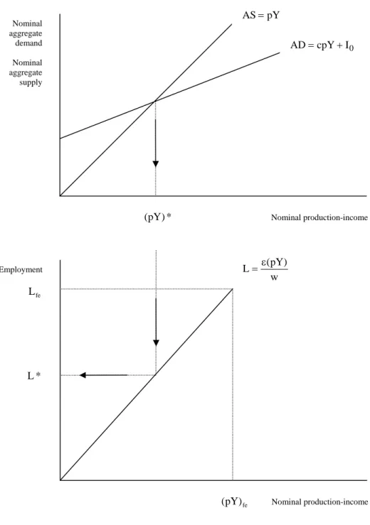
f < , such that Y=f(L). For sake of simplicity, let us assume f(L)= Lε with ε∈(0,1). Then, as described in Figure 2, the equilibrium between AD and AS determines a unique level of
maximum nominal production-income c 1 I )* pY ( 0 −
= , which is generally lower than (pY)fe. Note
that, unless the conditions of the aggregate demand (namely c and I ) change, a nominal 0 production-income level greater than (pY)* cannot be achieved because any situation where the nominal aggregate supply AS is higher than the nominal aggregate demand AD cannot be an equilibrium situation.
Further, let us assume that firms hire labour units according to the profit-maximization equality between real wage and marginal labour productivity, i.e. L 1
p
w =ε ε−
. Note that one can write the
latter condition as L L p w ε ε = or, alternatively, as w pY
L= ε , meaning that the equilibrium nominal
production-income (pY)* allows employing
w * ) pY ( *
L = ε individuals, a number of people that is generally lower than the number of people looking for a job L , as shown in Figure 2. So, the fact fe that I0 <Sfe determines the formation of unemployment in the amount of Lfe−L*.
To conclude, it is worth stressing that that the principle of effective demand is meaningless if the marginal propensity to consume is assumed to be equal to one. If this is the case, the monetary consumption expenditure is equal to the monetary production-income, i.e. C=pY, there are no monetary savings (S=0) at every production-income level including (pY)fe, no one dollar is left to be spent in investment goods (I0 = ), and the nominal aggregate demand 0 AD=C+I0 =pY coincides with the nominal aggregate supply AS=pY at every level of nominal production-income. Hence, every level of nominal production-income can be potentially achieved including the one corresponding to the full-employment level.
2. The principle of effective demand within the real wage vs. employment space
This section reviews the major contributions of the literature that tries to transfer Keynes’s principle of effective demand from the standard Samuelson’s space (in Figure 2) to the real wage vs.
employment space. Next section explores a simple extension of a model proposed by Lavoie (2003). Since there are many different equilibrium values in the paper, we adopt the strategy of marking equilibrium values with both a star and a number. The number refers to a specific model. Particularly, we distinguish among four different models: 1) the Patinkin-Barro-Grossman’s model, 2) the Davidson’s model, 3) the Lavoie’s model, 4) the extended Lavoie’s model.
Patinkin-Barro-Grossman’s model
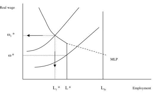
One of the first attempts of translating the principle of effective demand into the real wage vs. employment space is due to Patinkin (1956). Following the analysis of Patinkin, as summarized by Barro and Grossman (1971), the principle of effective demand translates into a labour-demand curve formed by two parts, as in Figure 3: a downward-sloping part, corresponding to the marginal labour-productivity schedule (MLP), and a vertical part intersecting the horizontal axis at the employment level L , as determined in the previous section. *
Formally, this labour-demand curve is derived by assuming that the production sector maximizes monetary profits under the constraint that the monetary aggregate supply cannot exceed the monetary aggregate demand, i.e. the production sector solves the following problem:
(3) AD AS t . s L wL ) L ( pf Max ≤ − = ∏
From an economic point of view, problem (3) means that the production sector hires labour units according to the profit-maximization rule f'(L)
p
w = until L<L* because the goods-market
) AD AS
( = and the production sector cannot hire additional labour units because additional workers (or working hours) would imply additional production remaining unsold.
The equilibrium levels of employment and real wage, in the Patinkin-Barro-Grossman’s model, are determined by the intersection between the labour demand and an upward-sloping labour supply, as shown in Figure 3. Let us label the level of employment as L1* and the level of the real wage as
* 1 ω .
Note that, if the labour-supply schedule shifts towards right as in Figure 3, then the equilibrium employment becomes *L and the equilibrium real wage becomes ω*, i.e. it is not equal to the marginal labour productivity at *L . Further, if the labour supply is assumed to be independent of the real wage and is modelled as a vertical line at the full-employment level L , then the fe equilibrium employment is given by *L and the excess of the labour supply pushes the equilibrium real wage down to the real value of the minimum wage.
It is worth stressing that the role played by the labour supply in determining the equilibrium levels of employment and real wage within the Patinkin-Barro-Grossman’s model is closer to the neoclassical tradition than to the (truly) Keynesian one. In addition, the fact that the model admits the possibility of an equilibrium, say (ω*,L*), where the real wage is not equal to the marginal labour productivity seems at odds with the original Keynes’s view.
Consistently with the true spirit of the Keynesian tradition, the models of the next subsections and the extended Lavoie’s model of the next section do not see any specific role played by the labour-supply curve in determining the equilibrium levels of employment and real wage, and the latter is equal to the marginal labour productivity.
Davidson’s model
Davidson (1983, 1994, 1998) closely follows the arguments that Keynes proposes in the Chapter 3 of The General Theory. In order to present the analysis of Davidson, let us again label the monetary wage as w and assume that the production function of the economy is specified as f(L)= Lε with
) 1 , 0 ( ∈
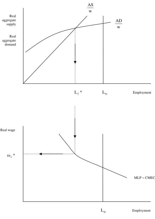
ε . Then, the level of employment is determined by the intersection, the so-called point of effective demand, between the real aggregate demand, expressed in units of money wages, i.e.:
(4) I0 w 1 cpL w 1 w AD = ε+
and the real aggregate supply, also expressed in units of money wages 1, i.e.:
(5) 1L
w AS
ε = .
Equation (4) is easily derived by (1). Indeed, expression (1) can be written as AD=cpY+I0 which is equivalent to AD=cpf(L)+I0, i.e. to AD=cpLε+I0. Hence, dividing both sides by the nominal wage w, we get (4).
Equation (5), instead, is derived by the profit-maximization equality between price and marginal cost, i.e. 1
L w
p ε−
ε
= , combined with (2). Specifically, 1
L w p ε− ε = is equivalent to 1 L wY pY ε− ε = , which is in turn equal to 1 L wL AS ε− ε ε = and finally to ε ε ε = L L L 1 w AS
. Since L cancels out, the latter ε
expression becomes equal to (5). Further details on the construction of the aggregate supply, both in real terms and in monetary terms, are provided by Davidson (1994, pp. 164-170).
The equality between (4) and (5) determines a unique equilibrium employment L2* in Figure 4, which does not necessarily coincide with the full-employment level L . fe
1
Measuring a given nominal amount in units of money wages simply means dividing this nominal amount by the
nominal wage rate w. The result is the real amount of labour units (either workers or working hours) that can be bought
As depicted in Figure 4, the real-wage level associated with L2* is determined by the marginal labour-productivity schedule, or the competitive market equilibrium curve (CMEC) as Davidson labels it, which gives the real-wage level implied by the level of employment determined by the point of effective demand, i.e. ω2*=ε(L2*)ε−1 where
p w =
ω is the real-wage level. Note that this
real-wage determination rule comes implicitly from the construction of the real aggregate supply, which starts from the equality between price and marginal cost and, therefore, from the equality between real wage and marginal labour productivity.
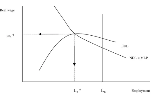
Lavoie’s model
Building on Davidson, Lavoie (2003) points out 2 that the quantity of labour and the real wage, associated with the point of effective demand, can be simply determined by the intersection between the so-called notional demand for labour (NDL), i.e. the marginal labour-productivity schedule (MLP), given by:
(6) ω=f'(L)
and the so-called effective demand for labour (EDL), given by f(L)=ωL+A or:
(7) L A ) L ( f − = ω
where A is real autonomous expenditure. Let us refer to the equilibrium pair of the Lavoie’s model in Figure 5 as ω and 3* L3*.
2
Expression (6), the notional demand for labour, is the standard profit-maximization condition stating that the real wage equals the marginal labour productivity. It is derived by assuming that the production sector optimally chooses the quantity of labour by maximizing nominal profits
wL ) L ( pf − = ∏ with respect to L.
Expression (7), the effective demand for labour, is derived by equating the aggregate supply in nominal terms AS=pf(L), in turn derived by (2), to the aggregate demand in nominal terms, given by:
(8) pAAD=wL+ .
To make the model as simple as possible, Lavoie (2003, p. 169) assumes that the nominal aggregate demand (8) is made up of only two components: nominal wages (wL), which are entirely consumed (the propensity to consume out of wages is equal to one), and nominal autonomous expenditures (pA), which cover both investments (I ) and consumption out of profits. 0
The aggregate demand (8) is therefore derived by (1) under the following three assumptions:
(A1) C=Cw+Cπ (A2) wLCw = (A3) pACπ+I0 =
where C is the nominal consumption expenditure of wage-earners, w C is the nominal π consumption expenditure of profit-earners, while A represents a given amount of real autonomous expenditures.
(9) ⎟ε ⎠ ⎞ ⎜ ⎝ ⎛ ε − = 1 3 1 A * L and ω3*=ε
(
L3*)
ε−1 ,meaning that the employment level is determined by the level of real autonomous expenditure A and by the labour elasticity of production ε.
From a pedagogical point of view, the Lavoie’s framework is useful because it allows to easily show that an increase in the real amount of autonomous expenditure A changes the location of the effective demand for labour without modifying its shape. Particularly, the effective demand for labour shifts downward and intersects the notional demand for labour in a new point of effective demand characterized by higher employment and lower real wage. Therefore, one can easily predict the labour-market effects of variations in the “animal spirits” of entrepreneurs.
In addition to the latter feature, the extended Lavoie’s model proposed in the next section also allows to predict the labour-market effects of a change in the propensity to save (consume) of income-recipients, which is interesting and important for two main reasons: first, as discussed in section 1, the principle of effective demand is meaningless if the marginal propensity to consume c of income-recipients is equal to one (i.e. the marginal propensity to save s is zero); second, as Figure 2 helps to show, variations of the propensity to consume (save) affect the slope of the nominal aggregate demand AD and imply variations of the nominal production-income level
* ) pY
( as well as variations of the employment level *L .
3. An extension of the Lavoie’s model
Let us start from the textbook presentation of the principle of effective demand where:
By the definition of aggregate nominal profits ∏=pY−wL, we obtain the following identity ∏
+ = wL
pY which can be replaced into (10), so that we get AD=c
(
wL+∏)
+I0 or alternatively0
I c cwL
AD= + ∏+ .
By further assuming that the propensity to consume of wage-earners c is, in general, different w from the propensity to consume of profit-earners c , we get the following general version of the π nominal aggregate demand AD=cwwL+cπ∏+I0 which in turn can be written as follows:
(11) AD=(1−sw)wL+(1−sπ)∏+I0
where )sw∈(0,1 is the propensity to save of wage-earners and sπ∈(0,1) is the propensity to save of profit-earners. It is worth stressing that expression (11), based on Mott and Slattery (1994), is not disregarded by Lavoie (2003, footnote 1), although not fully explored.
By equating (11) to the nominal aggregate supply AS=pY and using the definition of production function )Y=f(L , we obtain a general version of the effective demand for labour
0 w)wL (1 s ) I s 1 ( ) L (
pf = − + − π ∏+ , which can be re-written as follows:
(12)
(
)
L s s ) L ( f s w 0 − ζ − = ω π π where p I0 0 =ζ is real investment expenditure.
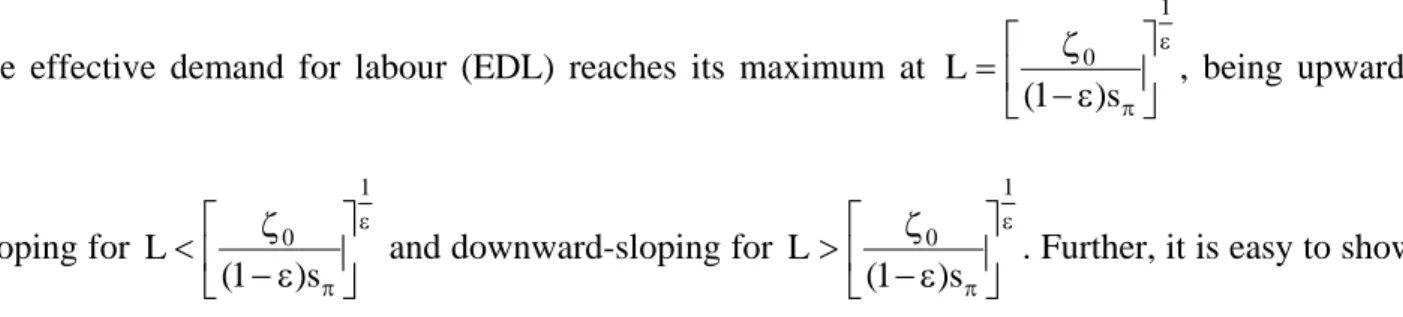
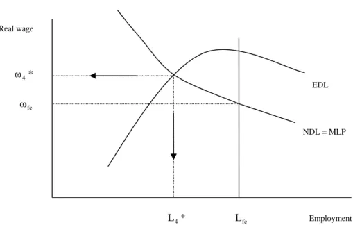
Expression (12) provides the locus of all the combinations of real wage and employment associated with the equilibrium in the market for goods. Regarding the shape of the effective demand for labour, let us again assume, as a matter of example, that f(L)= Lε. Then, as depicted in Figure 6,
the effective demand for labour (EDL) reaches its maximum at ε π⎥⎦ ⎤ ⎢ ⎣ ⎡ ε − ζ = 1 0 s ) 1 ( L , being upward-sloping for ε π⎥⎦ ⎤ ⎢ ⎣ ⎡ ε − ζ < 1 0 s ) 1 (
L and downward-sloping for ε
π⎥⎦ ⎤ ⎢ ⎣ ⎡ ε − ζ > 1 0 s ) 1 (
L . Further, it is easy to show
that that every point in the area below the effective demand for labour is characterized by excessive supply (AS>AD), while every point in the area above is characterized by excessive demand
) AD AS
( < .
The intersection between the effective demand for labour (12) and the notional demand for labour (6) gives the point of effective demand, i.e. the following pair:
(13) ε π ⎥⎦ ⎤ ⎢ ⎣ ⎡ ε + ε − ζ = 1 w 0 4 s s ) 1 ( * L and ω4*=ε(L4*)ε−1 .
It can be easily shown that 0 * L * 4 4 < ∂ ω ∂ , L * 0 0 4 > ζ ∂ ∂ , 0 s * L4 < ∂ ∂ π and 0 s * L w 4 < ∂ ∂ . Hence, an increase in
the real autonomous investment expenditure, an improvement of the “animal spirits” of entrepreneurs, increases the employment level and decreases the real wage, while an increase in the propensity to save of either wage-earners or profit-earners decreases the employment level and increases the real-wage level.
Figure 6 provides a useful framework for a comparison between the theory of employment developed by Keynes and the standard neoclassical theory. The labour-market equilibrium, in the neoclassical model, is given by the intersection between the notional demand for labour and the labour-supply schedule, which is assumed to be vertical for sake of simplicity. This intersection determines the real-wage level ω as well as the level of employment fe L , which is characterized fe by the absence of unemployment. The formation of unemployment Lfe−L4* is, instead, a specific
feature of the Keynesian point of effective demand, given by the intersection between the notional demand for labour and the effective demand for labour.
Note that the formation of unemployment in this type of Keynesian model does not rely on any assumption of wage rigidity (neither nominal nor real), in contrast to what is often claimed about Keynesian models.
Further, note that different models predict different outcomes of a policy stimulating the labour supply. In a neoclassical-type model, a shift towards right of the labour-supply schedule would increase the employment level by decreasing the real-wage level. In contrast, in the extended Lavoie’s model, such policy would increase the unemployment level without affecting the real-wage level.
4. Concluding note
Some Keynesian purists may disagree with the argument the principle of effective demand can be taught using the real wage vs. employment space as underlying framework. We share the view that the best way for teaching Keynes’s theory of employment consists of using The General Theory as main textbook reference for students, although this exercise is unlikely to be an appropriate exercise at undergraduate level.
References
Barro, J., and Grossman, H. (1971) A General Disequilibrium Model of Income and Employment, American Economic Review, 61(1), 82-93.
Dalziel, P., and Lavoie, M. (2003) Teaching Keynes’s Principle of Effective Demand Using the Aggregate Labor Market Diagram, Journal of Economic Education, 34(4), 333-340.
Davidson, P. (1983), The Marginal Product Curve is Not the Demand Curve for Labor and Lucas’s Labor Supply Function is Not the Supply Curve for Labor in the Real World, Journal of Post Keynesian Economics, 6(1), 105-117.
Davidson, P. (1994) Post Keynesian Macroeconomic Theory: A Foundation for Successful Economic Policies for the Twenty-First Century, Cheltenham: Edward Elgar.
Davidson, P. (1998) Post Keynesian Employment Analysis and the Macroeconomics of OECD Unemployment, Economic Journal, 108(448), 817-831.
Keynes, J.M. (1936) The General Theory of Employment, Interest, and Money, New York: Harcourt, Brace & Co.
Patinkin, D. (1956) Money, Interest, and Prices, Evanston: Row, Peterson & Co.
Lavoie, M. (2003) Real Wages and Unemployment with Effective and Notional Demand for Labor, Review of Radical Political Economics, 35(2), 166-182.
Mott, T., and Slattery, E. (1994) The Influence of Changes in Income Distribution on Aggregate Demand in a Kaleckian Model: Stagnation vs. Exhilaration Reconsidered, in: Davidson, P., and Kregel, J.A. (eds.) Employment, Growth and Finance, Aldershot: Edward Elgar.
Samuelson, P.A. (1948) The Simple Mathematics of Income Determination, in: Metzler, L.A. et al. (eds.) Income, Employment, and Public Policy: Essays in Honor of Alvin H. Hansen, New York: W.W. Norton & Co.
Figure 1. Nominal savings as lack of effective demand Nominal savings Nominal investments fe S I0 (pY)* (pY)fe Nominal production-income ) pY ( s S=
Figure 2. Samuelson’s model Employment fe L * L (pY)fe Nominal production-income w ) pY ( L= ε Nominal aggregate demand Nominal aggregate supply (pY)* Nominal production-income 0 I cpY AD= + pY AS=
Figure 3. Patinkin-Barro-Grossman’s model L1* L* Lfe Employment MLP Real wage * 1 ω ω*
Figure 4. Davidson’s model Real aggregate supply Real aggregate demand L2* Lfe Employment w AD w AS Real wage * 2 ω Lfe Employment MLP = CMEC
Figure 5. Lavoie’s model Real wage ω3* L3* Lfe Employment NDL = MLP EDL
Figure 6. Extended Lavoie’s model Real wage * 4 ω fe ω L4* Lfe Employment NDL = MLP EDL