Applied Mathematical Sciences, Vol. 9, 2015, no. 25, 1221 - 1228 HIKARI Ltd, www.m-hikari.com
http://dx.doi.org/10.12988/ams.2015.410808
Infinite Servers Queue Systems Busy Period -
A Practical Case on Logistics Problems Solving
J. A. Filipe1 and M. A. M. Ferreira
Instituto Universitário de Lisboa (ISCTE – IUL), BRU – IUL Lisboa, Portugal
Copyright © 2014 J. A. Filipe and M. A. M. Ferreira. This is an open access article distributed under the Creative Commons Attribution License, which permits unrestricted use, distribution, and reproduction in any medium, provided the original work is properly cited.
Abstract
In this paper it is exemplified how the busy period of an infinite servers queue is applied to the equipments failures management. With this model it is possible to obtain system performance measures and also to contribute to solve organizing structures’ problems, by minimizing the risks of the organizations inoperative structures, with considerable logistics pernicious consequences for companies and often also for the regions where the companies are inserted.
Keywords: Queue Model, Logistics, Equipments Management, Economic
Efficiency
1 Introduction
Situations of scarce resources demand very rigorous management rules. Structures management requires strong capabilities and competences. Solving logistics machine failures problems becomes crucial on this context.
In this model with MG queuing systems, customers arrive according to a Poisson process at rate 𝜆. Immediately after each one’s arrival, it receives a service which length is a positive random variable with distribution function G (.) and mean value 𝛼. An important system parameter is the traffic intensity . The service of a customer is independent from the other customers’ services and from the arrivals process. The busy period of a queuing system begins when a
1222 J. A. Filipe and M. A. M. Ferreira
customer arrives, finding it empty, and ends when a customer leaves the system letting it empty. During the busy period there is always at least one customer in the system. Formulae that allow the calculation of some of the busy period length parameters for the MG queuing system are presented in the next section. These results can be applied in Logistics (see, for instance [4, 5, 6, 10, 13], being the customers the failures occurred in the equipments. The service time in the queue is the time that a machine is idle waiting for reparation or being repaired. See also the operations cases in aircraft, shipping or trucking fleets in [9].
2 Some M
G
Queue System Parameters
In an MG queuing system there are neither losses nor waiting. In fact there is no queuing in the common sense. For these systems, to study the population process is not particularly important as for other systems with losses or waiting. Generally it is much more interesting the study of some other processes as, for instance, the busy period. The results related to the busy period length of the MG queuing system permit to find performance evaluation measures for the equipments. An illustration will be presented in this study, considering a very simple and short numerical example.
Being B the MG queuing system busy period length (see [8]), the mean value of B, whatever is G(.), is given in [15] as
e 1 B (2.1).Calling now VAR [B] to the variance of B, it can be seen that it depends largely on the form of B. Anyway in [14] it is stated that:
2
2 2 2 2 2 2 max e e s 2 e 1;0 VAR B 2e s 1 e 1 e 1 (2.2)wheresis the variation coefficient of G(.).
Considering now R(t) the mean number of busy periods that begin in [0,t] (being t = 0 the beginning of a busy period), after [2], it is possible to show that
𝑒−𝜌(1 + 𝜆𝑡) ≤ 𝑅(𝑡) ≤ 1 + 𝜆𝑡 (2.3), and that, see also [2], if the service time distribution function is G1(t) =
e−ρ
Infinite servers queue systems busy period 1223 VAR[B] =e2ρλ2−1, R(t) = 1 + λe−ρt (2.4); if it is G2(t) = 1 − 1 1−e−ρ+e−ρ+1−e−ρλ t , t ≥ 0 , VAR[B] =( eρ− 1)2 λ2 , R(t) = e−ρ+ (1 − e−ρ)2+ λe−ρt + e−ρ(1 − e−ρ)e−1−eλ−ρt (2.5).
Denote 𝑁𝐵 the mean number of the customers served during a busy period in the MG queuing systems. Considering the exposed in [3], if G (.) is
−𝐸𝑥𝑝𝑜𝑛𝑒𝑛𝑡𝑖𝑎𝑙 𝑁𝐵𝑀 = 𝑒𝜌 −𝐴𝑛𝑦 𝑜𝑡ℎ𝑒𝑟 𝑠𝑒𝑟𝑣𝑖𝑐𝑒 𝑑𝑖𝑠𝑡𝑟𝑖𝑏𝑢𝑡𝑖𝑜𝑛 𝑁𝐵≅ 𝑒 (𝜌(𝛾𝑠2+1))(𝜌(𝛾𝑠2+1)+1)+𝜌(𝛾 𝑠2+1)−1 2𝜌(𝛾𝑠2+1) (2.6).
A busy period is a period, in which there is at least one failure waiting for reparation or being repaired; and an idle period is a period in which there are no failures in the system.
Here some simple expressions - that allow computing the mean and bounds to the variance of the busy period - were given; and also simple bounds to the mean number of busy periods that begin in a certain interval time. Finally, expressions to the mean number of failures that occur in a busy period were also presented. These formulae are very simple and of evident application. They only require the knowledge of , , andsthat are very easy to compute. The only problem is to test the hypothesis that the failures occur according to a Poisson process.
Note yet that, calling I(t) the idle period of the MG queuing system distribution function, I(t) = 1 − e−λt, as it happens for any queue with arrival
Poisson process. In this application it gives the probability that the time length with no failures is lesser or equal than t.
3 A Short Numerical Case
Let’s suppose a fleet (or any machine’s system) where the failures occur at a rate of 20 per year. So λ = 20/year. Suppose also that the mean time to repair a failure is 4 days ( = 4 day = (4/365) year). In consequence 0.22.
1224 J. A. Filipe and M. A. M. Ferreira
Consider the possibility of decreasing to 0.11. Either making =10/year, for instance buying more items and decreasing, in consequence, each one use intensity. Or making = 2 day, for instance increasing the teams affected to the failures repairs.
On the contrary, if nothing is changed, things can get worse and maybe jump to 0.44. The values 0.88 and 12 are also considered.
If it is supposed that the repair services times are exponential3 s=1, and after
(2.1), (2.2), (2.3) and (2.6), with t=1 year, being SD[B] = √VAR[B],
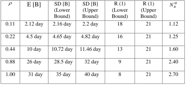
Table 1 Example for exponential service times
E [B]
SD [B] (Lower Bound) SD [B] (Upper Bound) R (1) (Lower Bound) R (1) (Upper Bound) M B N0.11 2.12 day 2.16 day 2.2 day 18 21 1.12
0.22 4.5 day 4.65 day 4.82 day 16 21 1.25
0.44 10 day 10.72 day 11.46 day 13 21 1.60
0.88 26 day 28.5 day 32 day 9 21 2.40
1.00 31 day 35 day 40 day 8 21 2.70
and it is possible to conclude, for these values, that when increases, less busy periods in one year occur, with more failures in each one, of course in mean values. The busy period mean and dispersion length also increase with.
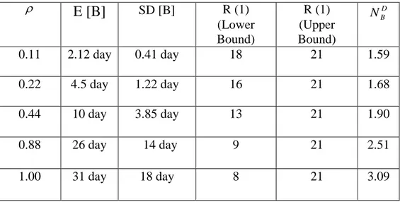
If it is supposed now that the repair service times are constant (D = deterministic), 0
s
, and after (2.1), (2.2)4, (2.3) and (2.6), with t = 1 year.
2 A neutral value for which the service rate equals the arrivals rate. 3 A very frequent supposition assumed for this kind of services.
Infinite servers queue systems busy period 1225
Table 2 Example for deterministic service times
E [B]
SD [B] R (1) (Lower Bound) R (1) (Upper Bound) D B N 0.11 2.12 day 0.41 day 18 21 1.59 0.22 4.5 day 1.22 day 16 21 1.68 0.44 10 day 3.85 day 13 21 1.90 0.88 26 day 14 day 9 21 2.51 1.00 31 day 18 day 8 21 3.09E [B] and the R (1) bounds are the same that in the former case, evidently. The behavior of the parameters with the increase ofis similar to the one of the exponential situation. But now the busy period length dispersion is much lesser and the mean value of failures in each busy period is greater.
As for the service times with distribution functions 𝐺1(𝑡) and 𝐺2(𝑡), it is not
possible to present results for 𝑁𝐵 because there is not an efficient formula to
calculate 𝛾𝑠. But 𝑆𝐷[𝐵] and 𝑅(1) are exactly calculated after (2.4) and (2.5) for
𝐺1(𝑡) and 𝐺2(𝑡), respectively.
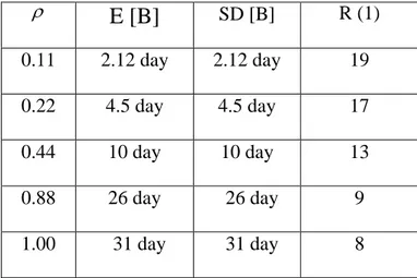
Table 3 Example for service times with 𝑮𝟏(𝒕) distribution function
E [B]
SD [B] R (1) 0.11 2.12 day 9.1 day 19 0.22 4.5 day 13.57 day 17 0.44 10 day 21.68 day 14 0.88 26 day 40 day 9 1.00 31 day 46.13 day 81226 J. A. Filipe and M. A. M. Ferreira
Table 4 Example for service times with 𝑮𝟐(𝒕) distribution function
E [B]
SD [B] R (1) 0.11 2.12 day 2.12 day 19 0.22 4.5 day 4.5 day 17 0.44 10 day 10 day 13 0.88 26 day 26 day 9 1.00 31 day 31 day 8Note that for G1(t) service time distribution function the busy period is exponentially distributed with an atom at the origin. For G2(t) service time distribution function the busy period is purely exponential. Anyway, in both cases, for these traffic intensity values, it is possible to conclude that the busy period mean and dispersion length also increase with.
4 Concluding Remarks
When operating a fleet5 managers are interested in big idle periods and little busy
periods. And if these busy periods occur they prefer that they are as rare as possible, with the shortest number of failures possible.
If he/she knows , , and sthe manager of the fleet can evaluate the quality of the operation, namely in terms of :
The mean length of a period with failures, The length dispersion of a period with failures,
The mean number of periods with failures that will occur in a certain length of time,
The mean number of failures that occur in a period with failures.
Infinite servers queue systems busy period 1227
As the expressions depend only on a few parameters, very simple to obtain and interpret, they show tracks to improve the operation, although they may be hard to implement depending on the company capabilities.
In the context of recent financial and economic crisis, numerical reliable indicators are very important because they allow defining good managing politics and practices. Besides their simplicity, the ones proposed in this paper own this reliability property.
References
[1] Carrillo, M. J., Extensions of Palm’s Theorem: A Review, Management Science, Vol. 37, n.º 6, p.739 – 744. 1991.
[2] Ferreira, M. A. M., Comportamento transeunte e período de ocupação de sistemas de filas de espera sem espera, PhD Thesis discussed in ISCTE, Supervisor: Prof. Augusto A. Albuquerque. 1995.
[3] Ferreira, M. A. M., Mean number of the Customers Served during a Busy Period in the MG Queueing System, Statistical Review, Vol. 3, INE. 2001. [4] Ferreira, M. A. M., Busy Period of Queueing Systems with Infinite Servers and Logistics, IMRL 2002 International Meeting for Research in Logistics. Proceedings (Volume-1), p. 270-274. 2002.
[5] Ferreira, M. A. M., M/G/ Queue Busy Period and Logistics, APLIMAT 2003. Proceedings (Part I). p. 329-332. 2003.
[6] Ferreira, M. A. M., Modelling and Differential Costs Evaluation of a Two Echelons Repair System through Infinite Servers Nodes Queuing Networks. Applied Mathematical Sciences, Vol. 7, Issue 109-112, 2013, p. 5567-5576. http://dx.doi.org/10.12988/ams.2013.38478
[7] Ferreira, M. A. M. and Andrade, M., MG Queue System for a particular Collection of Service Time Distributions. African Journal of Mathematics and Computer Science Research, Vol. 2, nº7. p. 138 - 141. 2009.
[8] Ferreira, M. A. M. and Andrade, M., “The Ties between the MG Queue System Transient Behavior and the Busy Period”, International Journal of Academic Research, Vol. 1, nº 1, p. 84-92. 2009.
1228 J. A. Filipe and M. A. M. Ferreira
[9] Ferreira, M. A. M., Filipe, J. A., Andrade, M., Coelho, M. Using infinite servers queue systems busy period to solve logistics’ problems. International Journal of Academic Research. Baku. Azerbaijan. 4 (3, PART A), p. 315-318. 2012.
[10] Ferreira, M. A. M., Andrade, M. and Filipe, J. A., Networks of queues with infinite servers in each node applied to the management of a two echelons repair system. China-USA Business Review, Vol. 8, nº 8, p. 39-45. 2009.
[11] Ferreira, M. A. M. and Filipe, J. A., Solving logistics problems using MG queue systems busy period, APLIMAT – Journal of Applied Mathematics. Vol. 3, nº 3. p. 207-212. 2010.
[12] Ferreira, M. A. M. and Filipe, J. A., Economic crisis: Using MG queue systems busy period to solve logistics problems in an organization, China-USA Business Review, Vol. 9, nº 9, p. 59-63. 2010.
[13] Ferreira, M. A. M., Filipe, J. A. and Coelho, M., Performance and Differential Costs Analysis in a Two Echelons Repair System with Infinite Servers Queues. Advanced Materials Research, Volume 1036, 2014, Pages 1043-1048, ModTech 2014 The Second International Conference on Modern Manufacturing Technologies in Industrial Engineering; Gliwice; Poland; 13 July 2014 through 16 July 2014.
http://dx.doi.org/10.4028/www.scientific.net/amr.1036.1043
[14] Sathe, Y. S., Improved Bounds for the variance of the busy period of the MG queue, A.A.P., p.913 – 914. 1985. http://dx.doi.org/10.2307/1427096 [15] Takács, L., An Introduction to queueing theory, Oxford University Press, New York. 1962.
Received: October 19, 2015; Published: February 17, 2015