Optimal Generalized Sequential Monte Carlo Test
I. R. Silva∗, R. M. Assun¸c˜ao
Departamento de Estat´ıstica, Universidade Federal de Minas Gerais, Belo Horizonte, Minas Gerais, Brazil
Abstract
Conventional Monte Carlo tests require the simulation ofm independent copies from the test statistic U under the null hypothesisH0. The execution time of these procedures can be substantially reduced by a sequential monitoring of the simulations. The sequential Monte Carlo test power and its expected time are analytically intractable. The literature has evaluated the properties of sequential Monte Carlo tests implementations by using some restrictions on the probability distribution of the p-value statistic. Such restrictions are used to bound the resampling risk, the probability that the accept/reject decision is different from the decision from the exact test. This paper develops a generalized sequential Monte Carlo test that includes the main previous proposals and that allows an analytical treatment of the power and the expected execution time. This results are valid for any test statistic. We also bound the resampling risk and obtain optimal schemes minimizing the expected execution time within a large class of sequential design.
Keywords: Sequential Monte Carlo test, Power loss, p-value density, Resampling risk, Sequential design, Sequential probability ratio test.
1. Introduction
In the conventional Monte Carlo (M C) tests, the user selects the number m of simulations of the test statisticU underH0. A Monte Carlo p-value is calculated based on the proportion of the simulated values that are larger or equal than the observed value of U, assuming that large values of U lead to the null hypothesis rejection. This procedure can take a long time to run if the test statistic requires a complicated calculation as, for example, those involved in complex models. These situations are exactly those where the MC tests are likely to be most useful, as analytical exact or asymptotic results concerning the test statistic U is hard to obtain. The adoption of sequential procedures to carry outM Ctests is a way to reach a faster decision. In contrast with the fixed sizeM C procedure, in the sequentialM C test the number of simulated statistics is a random variable. The basic idea is to stop simulating as soon as there is enough evidence either to reject or to accept the null hypothesis. For example, it is intuitively clear that, if the observed value of
∗Corresponding author
U is close to the median of the first 100 simulated values, the null hypothesis is not likely to be rejected even if we perform another 950 simulations. If a valid p-value could be provided, most researchers would be confident to stop at this point. Sequential Monte Carlo tests are procedures that provide valid p-values in these situations.
LetXtbe the number of simulated statistics underH0exceeding the observed valueu0att-th simulation.
In general, sequentialM C procedures track the Xt evolution by checking if it crosses an upper or a lower
boundary. When it does, the test is halted and a decision is reached. Typically, crossing the lower boundary leads to the rejection of the null hypothesis while the upper boundary crossing leads to the acceptance of the null hypothesis.
There are different proposals for a sequential Monte Carlo test in the statistical literature. Besag and Clifford (1991) proposed a very simple scheme that provides valid p-value for a sequential test with an upper bound n−1 in the number of simulations of U. It depends on a single tuning parameter h, making it extremely simple to use. We stop the simulations when Xt=hfor the first time andt < n. IfXn−1< h, the simulations are halted. Ifh≤l≤n−1 is the number of simulations carried out and if we stop at time t, the sequential p-value is given by
pBC =
Xt/t, ifXt=h,
(Xt+ 1)/n, ifXt< h.
(1)
The support set ofpBC is
S={1/n,2/n, . . . , h/n, h/(n−1), . . . , h/(h+ 2), h/(h+ 1),1} .
and we haveP(Ps≤a) =aunder the null hypothesis ifa∈S. This is a valid p-value estimator, because, a
p-value estimator Pe is valid ifP(Pe≤b)≤b, where bis an element from the support set ofPe. Additional
randomization can provide a continuous p-value with uniform distribution in the interval (0,1), rather than distributed on the discrete setS.
Therefore, the boundaries of Besag and Clifford (1991) are given by the horizontal line Xt = h and
the vertical line t = n−1. There is no lower boundary but only a predetermined maximum number of simulations, typically called a truncated sequential Monte Carlo test. The Besag and Clifford sequential M C test brings a reduction in execution time only when the null hypothesis is true. When it is false, one will often run the Monte Carlo simulation up to its upper boundn−1. Therefore, additional gains could be obtained by adopting a stopping criterium based on large values ofXt. For any fixed type I error probability
In addition to Besag and Clifford (1991), alternative sequential Monte Carlo tests have been suggested recently. These other procedures are mainly concerned with the resampling risk, defined by Fay and Follmann (2002) as the probability that the test decision of a realized M C test will be different from a theoretical M C test with an infinite number of replications. Fay and Follmann (2002) proposed the curtailed sampling design, where, if Xt ≥ ⌊α(n+ 1)⌋, the procedure is interrupted and H0 is not rejected, and, if t−Xt ≥ ⌈(1−α)(n+ 1)⌉ or the number of simulations reachesn, the procedure is interrupted and H0 is rejected, where n is the maximum number of simulations. They also introduced the interactive push out (IPO) procedure that requires a sequential algorithm to define the boundaries of the sequential procedure. This procedure is not proven to be optimal but simply to decrease the sample size with respect to a curtailed sampling design. For all their results, Fay and Follmann (2002) assumed a specific class of distribution for the p-value statistic, that distribution implied by a test statistic U that follows the standard normal distribution under the null hypothesis and follows aN(µ,1) under the alternative hypothesis. Conditional to this class of distributions, they found numerically the worst distribution to bound the resampling risk. IPO has a smaller expected execution time than the curtailed sampling design but its implementation is not practical for bounding the resampling risk in arbitrarily low values such as 0.01, for example. Also, we think that the assumption on the p-value distribution is too restrictive and, in fact, we show that it is not necessary to obtain optimal procedures.
Fay et al. (2007) proposed an algorithm (and an R package) to implement a truncated Sequential Prob-ability Ratio Test (tSPRT) to bound the resampling risk and studied its behaviour as a function of the p-value. The algorithm, denoted here as the FKH algorithm, calculates a valid p-value, which depends on the calculation of the number of ways to reach each point on the stopping boundary of the MC test.
Gandy (2009) proposed an algorithm to build a sequentialM Ctest that uniformly bounds the resampling risk in arbitrarily small values and provides lower bounds to the expected number of simulations. His algorithm is not truncated and the expected number of simulations can be infinite for p-values close to α. Therefore, the simulations may go on indefinitely. One missing issue in his paper is the lack of results concerning the type I error probability when the number of simulations is truncated.
Kim (2010) explored the approach from Fay and Follmann (2002) to bound the resampling risk using their same restrictive class of p-value distributions. She used the B-value boundaries proposed by Lan and Wittes (1988) and applied the algorithm of Fay et al. (2007) to obtain valid p-values estimates. She was able to obtain arbitrarily low bounds to the resampling risk and showed empirically that the B-value boundaries produces a smaller expected number of simulations than the IPO designs. In this paper, she also defined an approximated B-value procedure, which is easy to calculate and has analytical formulas that give insights on the choice of parameter values of the exact B-value design.
is the best alternative for a sequential MC test at the moment. However, its main results, concerning the resampling risk and the expected number of simulations, depend on the same restrictive class of p-value distributions of Fay and Follmann (2002). Moreover, important topics were not explored for the B-value boundaries such as, for example, its power with respect to the conventional M C test or the establishment of lower bounds for the expected number of simulations for any test statistic.
In this paper, we introduce a generalized sequential Monte Carlo allowing any monotonic shapes for the boundaries. For example, it is possible to construct boundaries which are close to each other in the beginning of the simulations, departing from each other as the simulations proceed and approaching each other again in the end of the simulations. We have been able to obtain bounds for the power loss of the sequentialM C test. In fact, we establish boundaries shapes such that the sequential M C test has the same power as the conventionalM C test for anyα level. These boundaries are simple to calculate and they are valid in the general case of any p-value distribution. Moreover, we are able to provide an algorithm to find the truncated boundaries that lead to a design with minimum expected sampling size. Concerning the resampling risk, we consider a larger class of distributions for the p-value than Fay and Follmann (2002) and we show that it is suitable to explicit algebraic manipulation allowing simple bounding of the resampling risk for any sequential M C test design.
This paper is organized in the following way. In the next section, we describe the B-value boundaries. Section 3 defines our sequentialM Ctest and develops its properties. In Section 4 we discuss a general class for the p-value distribution and provide some analytical results for the sequential tests. Section 5 presents a numeric routine for the preliminary choice of our boundaries and some specific suggestions for practical use. Section 6 offers a comparison between the B-value procedure and our procedure. Section 7 closes the paper with some discussion.
2. The B-value Procedure
Consider a hypothesis test of a null hypothesisH0 against an alternative hypothesisHa by means of a
test statistic U. The M C test can be seen as an estimation procedure to the unknown decision from the exact test based on the null hypothesis distribution of U. Kim (2010) has adopted this point of view by seeing the M C test as a decision procedure concerning in which (0,1) interval, either (0, α] or (α,1), does belong the exact p-value associated with the test statistic U. The parameter αis the significance level of the exact test. This interpretation leads to the following pair of hypotheses:
H∗
0 :p≤α
where p is the observed and unknown p-value generated from the random variable p-value. Viewed as a random variable, we denote the p-value by P. Clearly, the decision in favor of any hypotheses above leads to a decision concerning the original hypothesesH0 andHA.
LetUbe the test statistic,u0be its observed value for a fixed sample andui, i= 1, ...,be the independently
simulated values fromU underH0. Let
Xt= t X
i=1
1{[u0,∞)}(ui),
where 1{[u0,∞)}(ui) is the indicator function thatui≥u0.
Kim (2010) used the B-value introduced by Lan and Wittes (1988) to propose a sequential procedure to testH0∗ versusHA∗. Define:
V(t) =minns≥0 :x−tx≥c1pnα(1−α)o
and
L(t) =maxns≥0 :x−tα≤c2pnα(1−α)o .
Define also:
BSup =
(t, x) = (t,min{V(t), r1}) :t=t+0, t +
0 + 1, ..., n) , the upper boundary, and
BInf =
(t, x) = (t,max{L(t), t−r0}) :t=t−0, t−0 + 1, ..., n) ,
the lower boundary of a sequential Monte Carlo test, wheret+0 is the smaller value oft such that V(t)≤t and t−0 is the smaller value oft such that L(t)≥ 0. Similarly, let t+1 be the smaller value of t such that V(t)≥r1 andt−
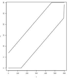
1 the smaller value oft such thatL(t)≤t−r0. The stopping boundaries from Kim (2010) are given by B=BInf∪BSup. TheB boundaries are formed by the union of linear functions int. Figure 1 illustrate the B-boundariesBSup andBInf usingc1=−c2= 1.282,n= 600 and α= 0.05.
The upper boundaryBSup is formed by the union of the line V(t) =c1 p
nα(1−α) +tα until t =t+1, when the upper boundary becomes the horizontal line with height r1 = ⌊α(n+ 1)⌋. The lower boundary BInf is formed by the line L(t) = c2
p
nα(1−α) +tα up to t = t−1 when it becomes the vertical line r0=t− ⌈(1−α)(n+ 1)⌉.
Kim (2010) usesφF KH, the test criterium based on the valid p-value presented in Fay et al. (2007). The
valid p-value is defined as ˆpv(Xt, t) =FˆpM LE(Xt/t), where ˆpMLE is the maximum likelihood estimator of p
and Fˆp is defined in (5.2) from Fay et al. (2007). The estimate ˆpv(Xt, t) of the p-value can be computed
using the FKH algorithm. The test adopted by Kim (2010) for theB boundaries is given by:
φF KH(t, x) =
1, if ˆpv(x, t)≤α
0 100 200 300 400 500 600
0
5
10
15
20
25
30
t
Xt
Figure 1: Example of theBboundaries withα= 0.05 and maximum number of simulations equal ton= 600.
When φF KH(t, x) = 0, H0 is not rejected (because H0∗ : p ≤ α is rejected). For φF KH(t, x) = 1, H0 is
rejected (that is,H∗
0 :p≤αis not rejected). Henceforth, this procedure is calledM CB.
It is very important to remark that there is no need to check the value of Xt at every momentt. To
see this, noticed that the boundariesBSup andBInf are composed by non-integer numbers while Xt is a
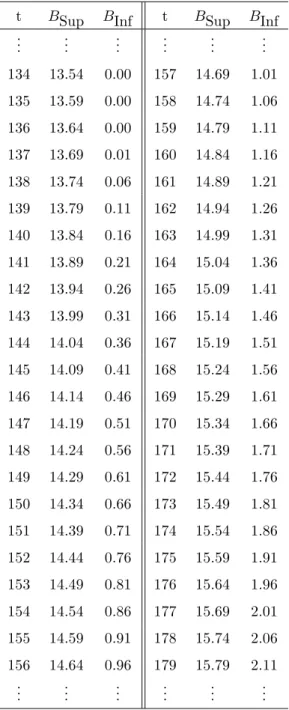
count. As a consequence, there will be timestfor which the simulations can not be interrupted byBInf and therefore there is no need to check against the lower boundary at these times. To illustrate this, consider the example from Kim (2010) illustrated in Figure 1. Table 1 shows the values ofBSup andBInf between the times 134 and 179. The lower boundary is equal to zero untilt= 136 and it is formed by numbers smaller than 1 untilt= 156. Therefore,Xtreach the lower boundary during this period ifX137= 0 and there is no
need to check against it fort≤136. Likewise, ifXtis not interrupted byBInf att= 156 (that is,X156≥2),
it will not reach it at least untilt= 176. Therefore, in practice, there is no need to check against the lower boundary for every simulated value. One needs to check only on those timest such that
BInf(t−1)< BInf(t)
for t = 2, . . . , m where BInf(t) is the value of the lower boundary at time t. This will be explored by our generalized sequential Monte Carlo method described in Section 3.
2.1. Bounding the resampling risk ofM CB
Fay and Follmann (2002) considered the IPO procedure that, interactively with the current simulations, adjusts the initial boundaries. This method allows the bounding of the resampling risk. The IPO procedure is not described in details here, but it should be noted that it is a computationally intensive procedure, and its implementation is intractable for bounding the resampling risk in arbitrarily small values (see (Kim, 2010)). Fay and Follmann (2002) considered a rather restrictive class of p-value distributions, with cumulative distribution function given by:
Hα,1−β(p) = 1−ΦΦ−1(1−p)−Φ−1(1−α) + Φ−1(β) (3)
where Φ(.) is the cumulative distribution function of a standard Normal distribution,αis the desired signif-icance level andβ is the type II error probability. Whenα= 1−β, the cumulative distributionHα,1−β(p)
has a uniform distribution on (0,1), as is expected whenH0 is true.
The p-value distribution defined in (3) assumes a variety of shapes, but the analytical manipulation of the resampling risk or of the expected number of simulations is intractable. To circumvent this problem, Fay and Follmann (2002) used a Beta(a, b) distribution to approximateHα,1−β(p), and this approximation
is denoted by ˜Hα,1−β(p). This approximation is chosen such that the expected value ofP coincides with
that fromHα,1−β(p) and such that ˜Hα,1−β(α) =Hα,1−β(α) = 1−β. Numerical studies were performed by
Fay and Follmann (2002) to obtain the worst case ˜F within the class (3) in the sense of having the largest resampling risk. Let ˜F∗ be the correspondent Beta distribution approximation to ˜F.
Although M CB is simpler and present a smaller expected time execution than the IPO procedure, it
depends on the FKH algorithm which requires rather complex modifications for each type of sequential design. Kim (2010) proposes an approximation for theM CB procedure. With this approximation, ifBSup
is reached before BInf, H∗
0 is rejected, while HA∗ is accepted if BInf is reached first. The approximation
may be used to gain analytic insights on the properties of the M CB procedure or to help on choosing the
parametersc1,c2, andn, as well as providing an approximation for the expected number of simulations. An undesirable characteristic of the approximated M CB is that it is not truncated and the expected number
of simulations must be calculated letting the maximum number of simulations go to infinity. Moreover, the approximation toM CB does not offer guarantee that the type I error probability is under control for any
choice ofc1 andc2. For this reason, the approximationM CB will not be explored here.
3. Our proposed generalized sequential Monte Carlo test
the terms associated with such number, and they used this algorithm to obtain both, the expected number of simulations and the resampling risk, for each fixed p-value. Fay et al. (2007) emphasize that such algorithm is valid only for the specific sequential procedure treated in that article, and adjustments are needed to use it with other sequential designs. Kim (2010) also used that algorithm for her calculations, and the approximate M CB is an attempt to escape from the dependence on special algorithms.
Aiming to overcome this limitation, we propose a truncated sequential procedure with two boundaries that have the shape of step functions. The values ofX(t) are checked against the upper boundary for every twhile they are checked against the lower boundary in an arbitrary set of predetermined discrete moments, possibly a smaller set than all integers between 1 andm. As we showed in Section 2, the B-boundaries can also be expressed by step functions with jumps equal to positive integer numbers. Therefore, the boundaries of M CB and of our sequential procedure can be expressed in the same way. To express the boundaries by
means of step functions is more cumbersome in terms of notation. The motivation for this design, where the lower boundary monitoring is not carried out for every timet, is mainly to allow for the analytical treatment of the power function, the expected number of simulations of the sequentialM C test for any test statistic. We also bound the resampling risk of our sequentialM C test.
LetηI =
nI
1, nI2, ..., nIk1 , withn I
j < nIj+1, be a set containing the moments when Xtmust be checked
against the lower boundary given by the values I = {I1, I2, ..., Ik1}. If XnIj < Ij, the simulations are
interrupted andH0 is rejected.
The monitoring ofXt with respect to the upper boundary crossing is carried out at all moments t =
1, . . . , mand this upper boundary is a step function. LetηS =
nS
1, nS2, ..., nSk2 , withn S
j < nSj+1be the jump moments for the upper boundary. FornS
j−1≤t < nSj, the upper boundary is given bySj wherenS0 = 0 and S1< S2. . . < Sk2. LetS ={S1, S2, ..., Sk2}. Therefore, the simulations are interrupted if Dt= 1, where:
Dt=
1, if (t∈ηI andX
t< Ij, for t=nIj) or (Xt=Sj, fornSj−1< t≤nSj)
0, otherwise (4)
or if the number of simulations reach a predetermined maximum equal tom.
Letxtbe the observed value of the random variableXt. The p-value can be estimated by:
pI =
xt/t, ifxt=Sj, nSj−1< t≤nSj
(xt+ 1)/(t+ 1), ifxt< Ij, t=nIj.
We define the test decision function for this sequential test:
φI(t, x) =
1, if the lower boundaryI is reached before the upperS or the simulations reachm 0, if the upper boundaryS is reached before the lowerI.
The hypothesis H0 is rejected if φI = 1 and it is not rejected if φI = 0. This sequentialM C test will be
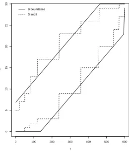
As an example, take k1 = k2 = 10, m = 600, and consider I = {0,1,2,3,9,15,20,24,27,29} for the lower boundary values,S ={5,7,9,13,17,23,26,29,29,30}for the upper boundary values, andηI =ηS = {20,50,79,119,239,359,459,539,569,600}. Figure 2 shows these boundaries as dashed lines.
The choice of the boundaries is closely linked to the desiredαmc, which is equal to 0.05 in this example.
In Section 5, we present an algorithm to obtain the appropriate boundaries for anyαmcandmin an easy and
fast way. The solid lines are theB boundaries calculated by Kim (2010) usingc1=−c2= 1.282,n= 600, andα= 0.05.
0 100 200 300 400 500 600
0
5
10
15
20
25
30
t
Xt
B boundaries
S and I
Figure 2: Example of the M CG(S and I) andBboundaries withα= 0.05 and a maximum number of simulations equal to
m= 600.
3.1. Power and Size of theM CG
In theM CG procedure, the rejection ofH0 occurs in the first moment t =nIj such that xt < Ij. The
power calculation is simpler if we merge the two sets ηI and ηS. Define η = ηI ∪ηS = {n1, n2, ..., n k}
with k = #η. Let S′ =nS1′, S ′ 2, ..., S
′
k o
be the upper boundary adjusted for each ni ∈η in the following
way. If ni =nSj ∈ ηS for somej, then S
′
i = Sj. If ni ∈ ηI ∩ ηS c
, then Si′ = Sj where j is such that
nS j = max
nS
r < ni . Thus, ifnimatches with some jump time in the setηS, thenS
′
iis equal to the value in
S for the timeni. Ifniis not an element inηS, thenS
′
i is the jump value of the time immediately preceding
ni.
Similarly, let I′ =nI1′, I ′ 2, ..., I
′
k o
be the adjusted lower boundary. That is, whenni =nIj ∈ηI or some
j, thenIi′ =Ij. Ifni∈ηS but ni∈/ ηI, thenI
′
i =Ij wherej is such that nIj = max
Thus, for a given value ofp∈(0,1), the power function of theM CG procedure, is given by:
πG(p) = I1′−1
X
x1=0
n1
x1
px1(1−p)n1−x1+
+
minnS′1−1,I
′
2−1
o
X
x1=I1′
minnI2′−x1−1,n2−n1
o
X
y=0
n2−n1
y
py(1−p)n2−n1−y×
× n1 x1
px1(1−p)n1−x1
+
+
k−1
X
j=2
minnSj′−1,Ij′+1−1
o
X
xj=Ij′
minnIj′+1−xj−1,nj+1−nj o
X
y=0
minnSj′−1−1,xj o
X
xj−1=Ij′−1 · · ·
· · ·
minnS′1−1,x2
o
X
x1=I1′
nj+1−nj
y × × n1 x1
py+xj(1−p)nj+1−y−xj j Y
i=2
ni−ni−1 xi−xi−1
. (5)
This expression is composed by ksummands. Ifk is not too large, the direct application of this expression produces results quickly and easily. The calculation would be computationally hard if we used a similar expression for sequential procedure where k = m. Note that, in the M CB procedure, the number of
summands in (5) can reach up to 2αmcm.
Under the null hypothesis,pfollows theU(0,1) distribution. Hence, by integrating out (5) with respect topwith aU(0,1) density, we obtain the type I error probability forM CG:
P(type I error) =
Z 1
0
πG(p)dp= I
′ 1 n1+ 1 +
+
minnS′1−1,I
′
2−1
o
X
x1=I1′
minnI2′−x1−1,n2−n1
o
X
y=0
n2−n1
y n1 x1
(n2+ 1)
n2
y+x1
+
+
k−1
X
j=2
minnSj′−1,Ij′+1−1
o
X
xj=Ij′
minnIj′+1−xj−1,nj+1−nj o
X
y=0
minnS′j−1−1,xj o
X
xj−1=Ij′−1 · · ·
· · ·
minnS′1−1,x2
o
X
x1=I1′
nj+1−nj
y n1 x1 Qj i=2
ni−ni−1 xi−xi−1
(nj+1+ 1)
nj+1 y+xj
Similarly to Silva and Assun¸c˜ao (2011), an upper bound for the power difference betweenM CG and the
exact test can be obtained by:
bG= max p∈(0,1)
1(0,α]−πG(p) (6)
whereαis the significance level of the exact test.
The power function of πG(p) evaluated for a fixed pis equal to the probability ofXtreachingI before
reachingS, and this probability is decreasing withp. In this way, the largest power loss ofM CGas compared
to the exact test is given by:
bG = max
p∈(0,α]{1−πG(α)}= 1−πG(α). (7)
Let M Cm be the conventional M C test performed with a fixed number m of simulations. An upper
bound for the power difference betweenM CmandM CG is given by:
bm,G= max
p∈(0,1){πm(p)−πG(p)} (8)
where πm(p) = P(G ≤ ⌊mαmc⌋ −1) is the power function of M Cm for a given p, and G is distributed
according to a binomial distribution with parametersm−1 andp.
3.2. Expected Number of Simulations forM CG
Let L be the random variable that represents the number of simulations carried out until the halting moment. To perform the computation of the expectation of L, obtained byE(L|P =p) = Pnk
l=1lP(L= l|P =p), for each fixedp. The probabilityP(L=l|P =p) is given by:
P(L=l|P =p) =
l−1 l−S1′
pl−S
′
1(1−p)S
′
1 ifl < n1
l−1 l−S1′
pl−S
′
1(1−p)S
′
1+PI
′
1−1 x=0 n1 x
px(1−p)n1−x ifl=n1
PI
′
1−1 x=0 n1 x1
l−n1−1 l−n1−(S2′ −x)
pS
′
2(1−p)l−S
′
2 ifn1< l < n2
PI
′
1−1 x=0 n1 x1
l−n1−1 l−n1−(S2′ −x)
pS
′
2(1−p)l−S
′
2+
Pmin
n
S1′−1,I
′
2−1
o
x=I′
1
Pmin
n
I2′−x−1,n2−n1
o
y=0
n2−n1
y
py(1−p)n2−n1−y×
× n1 x
px(1−p)n1−x
ifl=n2.
3, ..., k−1, we have:
P(L=l|P=p) =
minnSj′−1−1,I
′
j−1 o
X
xj−1=Ij′−1
minnIj′−xj−1−1,nj−nj−1
o
X
y=0
minnSj′−2−1,xj−1
o
X
xj−2=I′j−2 · · ·
· · ·
minnS1′−1,x2
o
X
x1=I1′
nj−nj−1 y × × n1 x1
py+xj−1(1−p)nj−y−xj−1 j−1
Y
i=2
ni−ni−1 xi−xi−1
+
+
minnSj′−1−1,I
′
j−1 o
X
xj−1=Ij′−1
minnSj′−2−1,xj−1
o
X
xj−2=Ij′−2 · · ·
· · ·
minnS1′−1,x2
o
X
x1=I1′
nj−nj−1−1 nj−nj−1−(S
′
j−xj−1)
× × n1 x1
pl−S
′
j(1−p)S
′
j
j−1
Y
i=2
ni−ni−1 xi−xi−1
.
Fornj−1< l < nj, j= 3, ..., k:
P(L=l|P =p) =
minnS′j−1−1,I
′
j−1 o
X
xj−1=Ij′−1
minnS′j−2−1,xj−1
o
X
xj−2=Ij′−2 · · ·
· · ·
minnS′1−1,x2
o
X
x1=I1′
nj−nj−1−1 nj−nj−1−(S
′
j−xj−1)
× × n1 x1
pl−S
′
j(1−p)S
′
j
j−1
Y
i=2
ni−ni−1 xi−xi−1
.
Finally, forl=nk:
P(L=l|P=p) =
minnSj′−1−1,I
′
j−1 o
X
xj−1=Ij′−1
minnIj′−xj−1−1,nj−nj−1
o
X
y=0
minnSj′−2−1,xj−1
o
X
xj−2=I′j−2 · · ·
· · ·
minnS1′−1,x2
o
X
x1=I1′
nj−nj−1 y × × n1 x1
py+xj−1(1−p)nj−y−xj−1 j−1
Y
i=2
ni−ni−1 xi−xi−1
Using thatphas a U(0,1) distribution under the null hypothesis, we have
E(L|H0 is true) =
Z 1
0
E(L|P =p)dp . (10)
To calculateE(L) underHA it is necessary to know the p-value distribution. However, a bound is easier
to calculate as
bE(L)=maxp∈(0,1){E(L|P =p)}. (11)
bE(L)is a very conservative upper bound forE(L). However, as we will illustrate in Section 5, this bound is useful to bound the expectation ofLin values less than 65% ofm.
4. A class of distributions for the p-value
Kim (2010) showed that, forp=α, the resampling risk is at least 0.5. Hence, it is not possible to bound the resampling risk in relevant values if we allow all distributions of p-values. This is the reason to define a class for the p-value distribution, taken as the setℑof all continuous probability distributions in (0,1) with differentiable densities that are non-increasing (that is, f′
P(p)≤ 0, for all p∈(0,1), with fP′ representing
the first derivative with respect topof the p-value density functionf.
From the p-value definition, its probability distribution function can be written in the following way:
P(P ≤p) = 1−FAF0−1(1−p) (12)
where FA denotes the probability distribution function of the test statistic U under HA and F0 is the
distribution ofU underH0.
Assuming the existence of densities functionsfA(u) and f0(u) ofU under HA andH0, respectively, the
p-value density can be written as:
fP(p) =
fAF0−1(1−p) f0
F0−1(1−p) . (13)
Hence, we can study the behavior of the p-value distribution by studying the behavior of the ratio between fA(u) andf0(u).
In the majority of the real applications, the ratio (13) is non-increasing withpand this is the motivation to restrict the analysis of the resampling risk to the set ℑ. Let ℑB be the class of p-value distributions
defined in Fay and Follmann (2002) with cumulative distributionHα,1−β(p), as described in Section 2. Let
πbe the power of the exact test. We will show now that, forπ≥α,ℑis more general thanℑB.
From the expression (3), the densitiesh(p)∈ ℑB can be indexed byαandβ and they are given by:
hα,1−β(p) = exp
−1
2
Φ−1(β)−Φ−1(1−α) Φ−1(β)−Φ−1(1−α) + 2Φ−1(1−p)
where Φ−1 is the inverse function of the standard normal cumulative distribution function Φ(·). The first derivative ofhα,1−β(p) with respect to pis equal to:
h′α,1−β(p) =
Φ−1(β)−Φ−1(1−α)
φ(Φ−1(1−p)) hα,1−β(p) (15)
whereφ(·) is the density function of the standard normal distribution. For 1−β≥α, we haveh′
α,1−β(p)≤0
for allp∈(0,1).
Consider the subset of densitiesℑ∗
B={fP(p)∈ ℑB: 1−β ≥α}. That is,ℑ∗B is a subset fromℑBformed
only by densities that implies an exact test power greater or equal toα. Therefore,ℑ∗
B ⊂ ℑ. Thus, at least
for useful test statistic (P(P ≤p)≥α), the classℑB is a particular case fromℑ.
The formulation of the classℑB in Fay and Follmann (2002) was inspired on the behavior of the p-value
distribution for the cases whereU0∼N(0,1) andUA∼N(µ,1), withµ= Φ−1(1−α)−Φ−1(β), which results
in a distribution with shapeHα,1−β(p). Fay and Follmann (2002) have explained that this same distribution
can be derived from the cases where U0 ∼ χ2
1(0) and UA ∼ χ21(µ2), where χ21(µ2) is the random variable with non-central Chi-square distribution with 1 degree of freedom and non-centrality parameter equal toµ2. They argued that, for the cases in whichU ∼F1,d(µ2) the p-value distribution converges in distribution to
Hα,1−β(p) whend→ ∞, whereF1,d(µ2) is the random variable withF distribution with 1 andddegrees of
freedom and non-centrality parameter equal toµ2.
The class ℑB is smaller thanℑ and does not cover all cases of interest. For example, the spatial scan
statistic developed by Kulldorff (2001) to detect spatial clusters follows very closely a Gumbel distribution under the null hypothesis and a chi-square distribution under HA (see Abrams et al. (2010)). Therefore,
even in interesting applied situations, there is not guarantee that fP(p)∈ ℑB and a larger class such as our ℑmay be useful.
It is worth mentioning that hα,1−β(p) is a convex function when 1−β ≥α and p≤ 0.5. Indeed, the
second derivative ofhα,1−β(p) with respect topis given by:
h′′α,1−β(p) =
Φ−1(β)−Φ−1(1−α)−φ′(Φ−1(1−p))
φ(Φ−1(1−p)) h
′
α,1−β(p) (16)
and we have that
φ′(Φ−1(1−p)) = Φ
−1(1−p)
√
2πφ(Φ−1(1−p))exp
n −1/2
Φ−1(1−p)2o
≥0
ifp≤0.5.
curve to the left hand, the convexity could not be verified forp≤0.5. For example, supposeU0 ∼χ2 1(0) e UA∼χ21,01(0). The corresponding p-value density from this conjecture is not concave forp >0.32.
The familyℑfor bounding the resampling risk is not restricted to families such as the normal, chi-square orF distributions. It also contains p-value densities with mixed shapes, with concave and convex parts. As an additional benefit,ℑallows the bounding of the resampling risk in a very simple way.
In the next subsections, we analyze the power, the expected number of simulations and the resampling risk of our generalized Monte Carlo test procedure when the p-value distribution belongs to the class ℑ. It is important to remember that, when using the M CG, the class ℑ is not needed neither to calculate a
bound for the power loss with respect to theM Cm or to the exact test nor to establish the bound for the
expected number of simulations under HA. Indeed, the results in the Sub-sections 3.1 and 3.2 are valid for
any test statistic. However, when the additional assumption that the p-value density fP(p) belongs toℑ
holds, stronger results can be obtained.
4.1. Upper bound for the power difference between the exact test and M CG
The power of the generalized Monte Carlo test is given by integrating out the probability πG(p) of
rejecting the null hypothesis conditioned on the p-valuepwith respect to the p-value density:
πG=
Z 1
0
πG(p)fP(p)dp .
The power difference between the exact test and M CG is given by:
δ∗G=
Z 1
0
1(0,αmc](p)−πG(p)
fP(p)dp. (17)
An upper bound forδ∗
I can be obtained if we usefP,w(p) = 1/αmcifp∈(0, αmc], andfP,w(p) = 0, otherwise:
δG∗ ≤b∗I =
Z 1
0
1(0,αmc](p)−πG(p)
fP,w(p)dp=
Z αmc
0 1 αmcdp−
Z αmc
0
πG(p)
1 αmcdp
= 1−α1 mc
Z αmc
0
πG(p)dp. (18)
Because the function (5) is a sum of Beta(a, b) density kernels, the integral (18) can be rewritten as a function of incomplete Beta(a, b) functions, all of them evaluated atp=αmc, witha andbdepending only
of the parameters I, S eη. In the same way, an upper bound for the power difference between M Cm and
M CG is given by:
b∗m,G=
Z αmc
0
(πm(p)−πG(p)) 1
αmcdp. (19)
4.2. An upper bound for the expected number of simulations
For values ofpnear 0, the simulation time is aroundn1, the first checking point of the lower boundary. For values ofpnear 1, the simulation time is aroundS1′, the smallest height of the upper boundary. Numerically, we find thatE(L|P =p) is maximized forparoundαmc. Let
pmax= arg max
p E(L|P =p)
and definefP,max(p) = 1/pmax, forp∈(0, pmax], and ¯fP,max(p) = 0, otherwise. Thus, it follows that
E(L) =
Z 1
0 E
(L|P =p) ¯fP(p)dp≤
Z 1
0 E
(L|P =p) ¯fP,max(p)dp=
Z 1/pmax
0 E
(L|P=p) 1
pmaxdp. (20)
The right hand side of the inequality (20) defines an upper boundb∗
E(L) forE(L).
4.3. An upper bound for the resampling risk
LetRRbe the resampling risk in a M C test defined as:
RR=Pmc(H0 is not rejected|P ≤α)P(P ≤α) +Pmc(H0 is rejected|P ≥α)P(P ≥α) (21)
where Pmc is the probability measure associated with the events generated by M C simulations. For the M CG test, denote its resampling risk byRRG, which is computed as:
RRG=
Z α
0
[1−πG(p)]fP(p)dp+
Z 1
α
πG(p)fP(p)dp. (22)
AsπG(p) is a decreasing function, the function1p∈(0,α](p)−πG(p)is maximum at p=α. Thus,RRG
is maximum when fP(p) puts the largest possible mass atα, which is the worst casefP,w(p). Substituting
fP(p) in (22) byfP,w(p) and settingα=αmc, we have :
RRG≤1−
1 αmc
Z αmc
0
πG(p)dp. (23)
Therefore, an upper bound forRRG is equal to the upper bound (18) for the power loss with respect to the
exact test. That is,b∗
RRG=b ∗
G.
The expression (22) can be rewritten in a way that emphasizes another property. The situation where π≥πG is that where the control ofRRG is important. Ifπ≥πG, then RRG≥δI, whereδI is the power
difference between the exact test and M CG. Therefore, equal power of the exact test and the M CG test
does not imply a null resampling risk. To see this:
RRG =
Z αmc
0
fP(p)dp− Z αmc
0
πG(p)fP(p)dp+
Z 1
αmc
πG(p)fP(p)dp
= π−πG+ 2
Z 1
αmc
πG(p)fP(p)dp=δI+ 2
Z 1
αmc
5. Choosing Parameters to Operate M CG
This section aims to provide the reader with a useful set of choices for the parametersI,S andη to run theM CG test. The choices we suggest produce aM CG test with power equal to aM Cm test for any test
statistic with small expected number of simulations.
OptimizingE(L) analytically is undoubtedly a complex task. In contrast, a numeric approach is feasible and simple to operate, and this is the approach adopted here. Define the classM, the set ofM CGprocedures
that, under H0, leads to the same decision about rejecting H0 than theM Cm. Conditioned on this class
M, the three next steps were developed to estimate the parameters of the M CG with minimum E(L). Let
M CIop be such scheme with minimumE(L).
1. This step is intended to emulate the Xt path under H0. Generate N observations from an U(0,1)
distribution, and label them aspi, i= 1, ..., N. For eachpi, generatemvaluesxij, with j= 1, . . . , m
following a Bernoulli distribution with success probabilitypi. Define the partial sum processes
Si= (
Sit, such thatSit= t X
l=1
xil, t= 1, ..., m )
.
2. We build envelopes for the path Xt based on the simulated ones. For that, select those Si
se-quences leading to the rejection ofH0 byM Cm. That is, to be selected the sequenceSi must satisfy
maxt{Sit}< mαmc. Suppose there aresof those sequences and they form the setR. IfN is large, we
expect s/N ≈αmc. Define the sequence ˆSt ={maxi{Sit}+ 1, i∈ R}. The curve ˆSt is an estimator
for the upper boundary ofM CGop.
Next, take ther sequencesSi such that maxt{Sit} ≥mαmc and collect them in the setA. These are
the sequencesS′
isthat do not rejectH0. Define the sequence ˆIt={mini{Sit}, i∈ A}. The curve ˆItis
the estimator for the lower boundary ofM CGop.
3. Take the set ˆηS containing the jumping moments of ˆS. ˆηS is an estimator forηS associated toM C Gop.
Take also the set ˆηI formed by the jumping moments of ˆI. ˆηI is an estimator of ηI associated to
M CGop. Formally:
ˆ ηI =nnˆI
t = ˆnIt−1if
l
ˆ It
m
=lIˆt−1
m
, or ˆnIt =t if l
ˆ It m
>lIˆt−1
mo
(25)
with,t= 2, ...., mand ˆnI
1= min
n
l: ˆIl>0 o
, l= 1, ..., m. Also,
ˆ
ηS =nˆnS
t = ˆnSt−1if
j
ˆ St⌋ =
j
ˆ
St−1⌋, orˆnSt =t if j
ˆ St⌋ >
j
ˆ
St−1⌋(26)
with,t= 2, ...., mand ˆnS
1 =min
n
ˆ St
o
. The estimation procedure ends here.
0 200 400 600 800 1000
10
20
30
40
50
t
Xt
E1
Estimated I and S
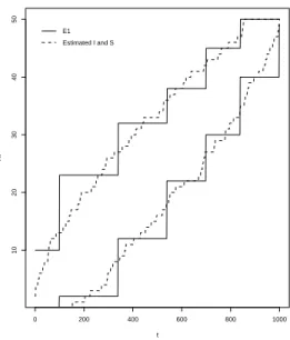
Figure 3: SchemeE1 from Table 5 versus estimates for I and S consideringm= 1000,N= 100000 andαmc= 0.05
that, underH0, the decision of theM CG will be always the same as that reached withM Cm. In addition,
iffP(p)∈ ℑ, we have
P(XtreachI before reachS |H0)≤P(Xt reachI before reachS |HA),
and then the power of these estimated boundaries is, at least, equal to that from M Cm. Concerning the
expected number of simulations, E(L) decreases by increasing the I elements and by decreasing the S elements. The construction of ˆSt and ˆIt follows this logic. The reasoning is to scan each t taking the
maximum value forIwhich does not restrict the Xttrajectories which would not rejectH0 by usingM Cm.
Simultaneously, it takes the minimum value for S which does not restrict the Xt trajectories which would
rejectH0by usingM Cm.
The resulting estimators of ηI and ηS are quite sparse using this algorithm, while they could be
com-putationally costly if calculated by means of the expressions developed in Section 3. An alternative and satisfactory way to construct ηI and ηS is based on the identification of the moments with high incidence
of impact ofXt with the estimated boundaries. For that, letn∗q = min n
t∈[1, ..., m], t:Sit≤I, iˆ ∈ R o
be an element of the sequence formed by the impact moments of each sequence Sit with ˆI (considering only
those sequencesi∈ R). The most frequent impact moments of these sequencesSit with ˆI are appropriate
candidates for composingηI. Apply the same reasoning for constructingηS, and denote the correspondent
sequence byn∗
r. Thus, as an alternative way to constructηI andηS, by arbitrary and conveniently low values
k1 and k2, choose the most frequent elements in n∗
q and n∗r to composeηI andηS, respectively. Extensive
of simulations have a small computational cost, and the results are close to that using ˆηI and ˆηS.
Figure 3 shows the estimates ˆI and ˆS obtained according to the steps 1, 2, and 3, of our algorithm, using N = 100000, m = 1000 and αmc = 0.05. The estimated boundaries are not parallel, but they are
characterized by a funnel in the extremities. This behavior was verified in all of the simulations performed by us. For these specific estimates, if we takeη=ηS =ηI, we obtain the times ˆη={99,339,539,699,839,999}.
From the estimates plotted in Figure 3, we obtain ˆI={2,12,22,30,40,49}, and ˆS={10,23,32,38,45,50}. This specific scheme for our generalized sequentialM C test is available in Table 5 and it is labeled asE1. As we can see in the Table 2, column bm,I, this scheme is efficient, presenting practically the same power
than M Cm for m= 1000, with size equal to 0.049864. From Table 3, columnsE(L|H0) and bE(L), we see
that this scheme have a small expected number of simulations, equal to 58.606 underH0, and with an upper bound underHA for any statistic, that is approximately 65% of the maximum 999. By using the classℑB
and the larger class ℑ for the p-value distribution, the bounds are expressively low, equal to 172.612 and 246.354, respectively. We consider that this scheme is a good option to replaceM Cm. We must enphasize
that, although the boundaries presented in Table 5 were guided by the algorithm above, all results in tables 2 and 3 are exact, because they were obtained by applying the expressions from Sections 3 and 4. Such algorithm is useful to construct preliminary choices of boundaries. The validation of an arbitrary design to practical use must be based on such exact calculations.
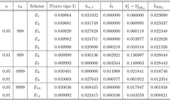
We provide other interesting schemes in Table 5. For each scheme, Table 2 offers the type I error probability, the upper bound for the power loss comparatively toM Cmand to the exact test, and the upper
bound for the resampling risk. Table 3 gives the expected number of simulations under H0 and the upper bounds under HA. We adopt bm,G to denote the general upper bound for the power loss comparatively
to M Cm, b∗G and b∗RRG, the upper bounds for the power loss, with respect to the exact test, and for the
resampling risk, respectively, where the super index ∗ indicates that the calculations are restricted to the p-value distribution on the classℑ. The same symbol was used to indicate the use of this class for the bounds in Table 3. Upper bounds using the classℑB are also available in Tables 2 and 3, and they are indicated by a tilde accent. Concerning the use ofℑB, the numerical explorations of Fay and Follmann (2002) were not used here to define the worst case of a p-value distribution with shape Hα;1−β(p). As discussed in Section
4.3,hα,1−β(p) (for 1−β≥α) andπG are decreasing with p. Therefore, the worst case within the classℑB,
in the sense of boundingRRI, occurs at the point of maximum of the function Hα;1−β(α) with respect to
β. For 1−β≥α, the point of maximum inβ for the functionHα;1−β(α) is 0.5. Then, the analytical worst
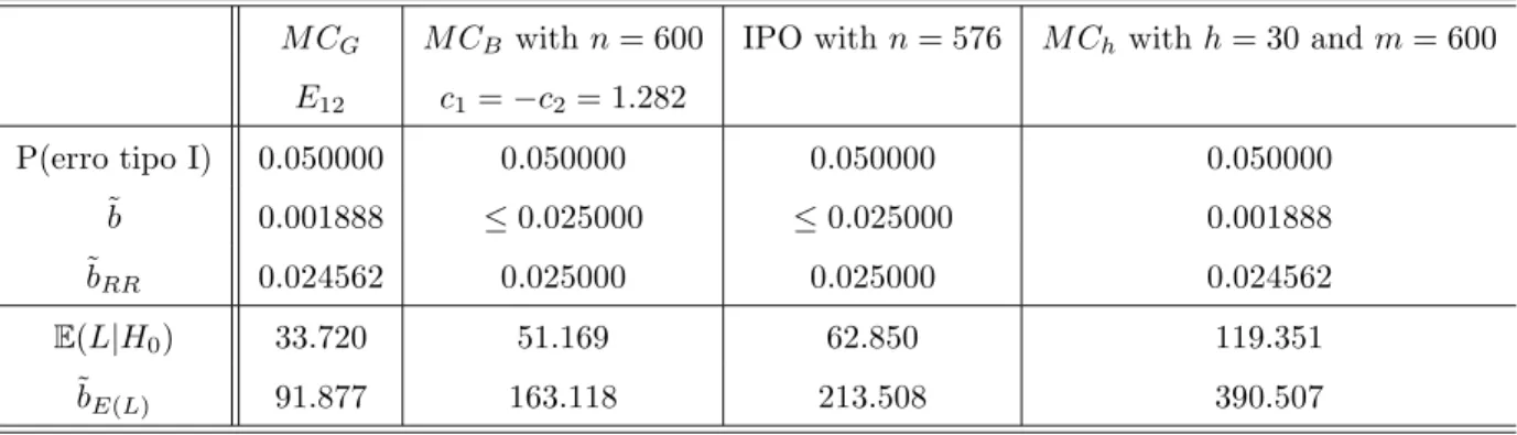
6. M CG versusM CB
In this Section we offer a comparison between theM CBandM CGsequential test procedures. We use an
example of theM CB test given by Kim (2010). In this comparison, we focus on resampling risk bound and
on the expected number of simulations. We assume that the p-value distributionfP(p) belongs to the class ℑB. We did not consider other important characteristics of a test, such as the power loss with respect to the exact test and expected number of simulations for an arbitraryfP(p), because they were not treated by Kim
(2010). We built ourM CG boundaries using the algorithm from Section 5. After securing an upper bound
for the resampling risk to M CG equal to that presented by theM CB scheme developed in Kim (2010), we
compared the average simulation time of the two procedures.
An obvious fact is that theBboundaries are particular cases ofIandS, becauseM CG was designed to
be a generalized sequential with two stopping boundaries. We can rewrite theB boundaries using theM CG
notation, based on the sets I, S, ηI andηS. In this way, for an M C
B test, the user can apply the general
expressions for the power and the expected number of simulations developed in Section 3. Define:
T1∗=
t >2 :
BInf(t−1)
<
BInf(t)
and
T2∗=
n
t >2 :jBSup(t−1)k<jBSup(t)ko .
Lett∗
11< t∗12< ... < t∗1k1 be the ordered elements of T
∗
1, andt∗21< t∗22< ... < t∗2k2 be the ordered elements
of T2∗. Rewritten in terms of I andS, the B boundaries are denoted by I∗,S∗, ηI∗ andηS∗, and they are built as follows:
I∗=
⌈BInf(t∗11)⌉,⌈BInf(t∗12)⌉, ...,
BInf(t∗1k1)
S∗=
⌊BInf(t∗21)⌋,⌊BInf(t∗22)⌋, ...,
BInf(t∗2k2)
ηI∗=
t∗11, t∗12, ..., t∗1k1
ηS∗=
t∗21, t∗22, ..., t∗2k2 .
It should be noted that some important shapes forIandS, as the funnel behavior estimated in Section 5, can not be represented by theM CB boundaries.
0 100 200 300 400 500 600
0
5
10
15
20
25
30
A
t
Xt
MCB
MCG
0 100 200 300 400 500 600
0
5
10
15
20
25
30
B
t
Xt
MCB
I and S est
0 100 200 300 400 500 600
0
5
10
15
20
25
30
C
t
Xt
MCG
I and S est
0 100 200 300 400 500 600
0
5
10
15
20
25
30
D
t
Xt
MCB
MCG
I and S est
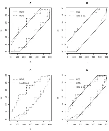
Figure 4: Boundaries forM CGandM CB sequential test procedures.
using the scheme E12 detailed in Table 5. Concerning the worst case of distribution within the class ℑB, Kim (2010) adopted the numerical studies from Fay and Follmann (2002) and she found ˜F∗=H0
.05;0.47(p)
forα= 0.05, with approximation ˜H0.05;0.47(p) :=Beta(0.389; 2.523).
These bounds are also computed here for the sequential procedure proposed by Besag and Clifford (1991), which will be denoted byM Ch. ThisM Chprocedure is a very simple way to perform sequential tests, because
it is based just in an upper boundary fixed in a value denoted byhand truncated in a maximum number of simulations n. Silva et al. (2009) had showed that M Ch has the same power than M Cm ifh =αmcm
and its power is constant forn≥h/αmc+ 1, noting that the combination of this two last rules implies that
M Cmmust be replaced byM Ch, because they have the same power for a maximum number of simulations
practically equal (that is, forn=m+ 1).
Under either hypothesis,M CGis substantially faster than theM CB procedure with their expected time
ratio being around 60%. This illustrates the gain provided by ourM CGalgorithm. The estimated boundaries
form= 600 and αmc= 0.05 for the M CG procedure are available in Figure 4, where we can also see theB
given by theM CGboundaries. While theB boundaries are parallel almost up to the end of the experiment,
the I and S boundaries are tapered when t gets close to the maximum number of simulations. This can be intuitively thought as if the boundaries were using the information thatXt not touching the boundaries
after a long time was inducing a narrower vigilance.
7. Discussion
The generalized sequential Monte Carlo test has properties that recommend it in substitution to the conventional Monte Carlo test for any test statistic. In this paper, we gave simple expressions for the calculation of the test size, the expected number of simulations under the null hypothesis, and upper bounds for the expected number of simulations under the alternative hypothesis and for the power loss with respect to the fixed length conventional Monte Carlo test.
t BSup BInf t BSup BInf ..
. ... ... ... ... ... 134 13.54 0.00 157 14.69 1.01 135 13.59 0.00 158 14.74 1.06 136 13.64 0.00 159 14.79 1.11 137 13.69 0.01 160 14.84 1.16 138 13.74 0.06 161 14.89 1.21 139 13.79 0.11 162 14.94 1.26 140 13.84 0.16 163 14.99 1.31 141 13.89 0.21 164 15.04 1.36 142 13.94 0.26 165 15.09 1.41 143 13.99 0.31 166 15.14 1.46 144 14.04 0.36 167 15.19 1.51 145 14.09 0.41 168 15.24 1.56 146 14.14 0.46 169 15.29 1.61 147 14.19 0.51 170 15.34 1.66 148 14.24 0.56 171 15.39 1.71 149 14.29 0.61 172 15.44 1.76 150 14.34 0.66 173 15.49 1.81 151 14.39 0.71 174 15.54 1.86 152 14.44 0.76 175 15.59 1.91 153 14.49 0.81 176 15.64 1.96 154 14.54 0.86 177 15.69 2.01 155 14.59 0.91 178 15.74 2.06 156 14.64 0.96 179 15.79 2.11
..
. ... ... ... ... ...
α nk Scheme P(erro tipo I) bm,I ˜bI b∗I =b∗RRG ˜bRRG
E1 0.049864 0.031032 0.000000 0.060000 0.023000 E2 0.049681 0.031748 0.000000 0.060895 0.023337 0.05 999 E3 0.049920 0.027828 0.000000 0.060118 0.022348 E4 0.049982 0.024751 0.000000 0.053977 0.022826 E5 0.049998 0.020890 0.000218 0.058518 0.021326 0.01 999 E6 0.009999 0.030136 0.002921 0.136997 0.028048 E7 0.009993 0.000000 0.003344 0.140063 0.028443 0.05 4999 E8 0.050401 0.000000 0.014908 0.021841 0.016746 0,01 E9 0.010003 0.027643 0.000577 0.061952 0.012354 0.05 9999 E10 0.050036 0.008435 0.000000 0.017947 0.001838 0.01 E11 0.009992 0.023415 0.000106 0.043559 0.008821
Table 2: Effective test size, upper bound for the power loss, and for the resampling risk associated to the schemes in the Table
5.
α nk Scheme E(L|H0) bE(L) ˜bE(L) b∗E(L) E1 58.606 644.654 172.612 246.354 E2 96.739 807.572 235.119 402.704 0.05 999 E3 113.597 792.104 264.587 407.943 E4 108.472 670.761 276.496 396.895 E5 128.276 698.242 335.969 474.473 0.01 999 E6 42.717 677.409 225.362 550.574 E7 41.728 625.841 225.334 523.601 0.05 4999 E8 384.591 4283.575 1016.884 1716.704 0.01 E9 121.992 3580.891 1816.592 687.744 0.05 9999 E10 731.131 9477.250 1951.502 3502.344 0.01 E11 190.355 8706.908 1182.462 3968.661
M CG M CB withn= 600 IPO withn= 576 M Ch withh= 30 andm= 600
E12 c1=−c2= 1.282
P(erro tipo I) 0.050000 0.050000 0.050000 0.050000
˜b 0.001888 ≤0.025000 ≤0.025000 0.001888
˜
bRR 0.024562 0.025000 0.025000 0.024562
E(L|H0) 33.720 51.169 62.850 119.351
˜bE(L) 91.877 163.118 213.508 390.507
Table 4: Upper bounds for the resampling risk and expected number of simulations for comparison amongM CGusingE12,
I={2,12,22,30,40,49}
E1 S={10,23,32,38,45,50}
η={99,339,539,699,839,999}
I={2,12,20,35,49}
E2 S={19,30,37,45,49}
η={99,379,539,779,999}
I={7,16,24,35,49}
E3 S={28,35,41,49,49}
η={199,499,699,899,999}
I={13,22,30,35,49}
E4 S={28,35,42,45,49}
η={299,559,719,799,999}
I={17,26,35,42,49}
E5 S={34,39,43,46,49}
η={399,639,799,899,999}
I={1,5,7,8,9}
E6 S={8,9,9,9,9}
η={299,599,799,899,999}
I={2,5,7,8,9}
E7 S={8,8,8,9,9}
η={399,599,769,899,999}
I={27,100,199,249}
E8 S ={80,150,219,249}
η={799,2499,3999,4999}
I={5,20,35,49}
E9 S={20,31,43,49}
η={799,2499,3999,4999}
I={17,79,499}
E10 S={79,249,499}
η={499,2999,9999}
I={79,199,499}
E11 S={199,499,499}
η={2399,4999,9999}
I={0,1,2,3,9,15,20,24,27,29}
E12 S={5,7,9,13,17,23,26,29,29,30}
References
Abrams, A., Kleinman, K., Kulldorff, M., 2010. Gumbel based p-value approximations for spatial scan statistics. International Journal of Health Geographics 9 (61).
Besag, J., Clifford, P., 1991. Sequential monte carlo p-value. Biometrika 78, 301–304.
Fay, M., Follmann, D., 2002. Designing monte carlo implementations of permutation or bootstrap hypothesis tests. The American Statistician 56 (1), 63–70.
Fay, M., Kim, H.-J., Hachey, M., 2007. On using truncated sequential probability ratio test boundaries for monte carlo implementation of hypothesis tests. Journal of Computational and Graphical Statistics 16, 946–967.
Gandy, A., 2009. Sequential implementation of monte carlo tests with uniformly bounded resampling risk. Journal of the American Statistical Association 104 (488), 1504–1511.
Kim, H.-J., 2010. Bounding the resampling risk for sequential monte carlo implementation of hypothesis tests. Journal of Statistical Planning and Inference 140, 1834–1843.
Kulldorff, M., 2001. Prospective time periodic geographical disease surveillance using a scan statistic. Journal of Royal Statistical Society 164A, 61–72.
Lan, K., Wittes, J., 1988. The b-value: a tool for monitoring data. Biometrics 44, 579–585.
Silva, I., Assun¸c˜ao, R., 2011. Monte carlo test under general conditions: Power and number of simulations. Paper submitted to Journal of Statistical Planning and Inference.
Silva, I., Assun¸c˜ao, R., Costa, M., 2009. Power of the sequential monte carlo test. Sequential Analysis 28 (2), 163–174.
Acknowledgements