Modeling of an Autonomous Underwater Vehicle

(1)

UNIVERSITY OF BEIRA INTERIOR

Engineering

Modeling of an Autonomous Underwater Vehicle

Cristiano Alves Bentes

Thesis submitted in fulfillment of Master Degree in

Aeronautical Engineering

(Integrated Cycle of Studies)

Academic Supervisor: Professor Kouamana Bousson

(2)

(3)

Dedication

To my parents, Maria Fernanda Veigas Alves and João Jaime Bentes, for all the support and dedication.

To my family and friends who have always been there for me.

”My momma always said, ”Life was like a box of chocolates. You never know what you’re gonna get.””

(4)

(5)

Acknowledgments

Thank you to my academic supervisor Professor Kouamana Bousson for all the dedication and support.

My utmost gratitude to my co-supervisor, Tiago Rebelo, and all the engineers at CEiiA, who provided much needed guidance and support during my internship.

My absolute gratitude to my parents, Fernanda and João, for their unconditional love and sup-port.

A special thanks Maria, Lucy and Serra, for their friendship.

(6)

(7)

Resumo

Os veículos subaquáticos autónomos (Autonomous Underwater Vehicles – AUV’s) têm múltiplas aplicações militares, comerciais e para investigação científica. A grande vantagem destes veícu-los advém da sua independência, sendo que operam sem a necessidade de supervisão humana. No entanto esta capacidade implica que os sistemas de navegação, guia e controlo sejam com-pletamente responsáveis pelo governo do veículo. O sistema de controlo destes veículos é tipi-camente projetado tendo como base um modelo dinâmico do mesmo. Este modelo pode ser também usado para simulação e análise de desempenho. O propósito deste trabalho é desen-volver um modelo dinâmico para um AUV de investigação de duplo-corpo, a ser desenvolvido no CEiiA.

Dado que o objetivo principal do modelo é projetar controladores e, de modo a fornecer várias abordagens para o efeito, os respetivos modelos (subsistemas) lateral e longitudinal são de-duzidos. Estes modelos são posteriormente validados através da comparação de resultados de simulação para os subsistemas com os resultados de simulação para o modelo completo. A modelação deste veículo é efetuada usando o modelo dinâmico de Fossen. Este modelo pode ser dividido em cinemática e cinética. Cinemática aborda os aspetos geométricos do movimento. As equações de cinemática são fornecidas tanto para ângulos de Euler como para quaterniões. As equações de cinética centram-se na relação entre movimento e força. O modelo de Fossen identifica quatro forças distintas que influenciam a dinâmica dos veículos subaquáticos: forças de corpo rígido; forças hidrostáticas; amortecimento (atrito) hidrodinâmico e added mass. Es-tas forças são modeladas através de métodos analíticos e computacionais. O modelo CAD do veículo, desenvolvido pelo CEiiA, foi usado para estimar os parâmetros de massa e inércia, bem como forças hidrostáticas. O amortecimento hidrodinâmico foi estimado através da adaptação de análises CFD, também efetuadas pelo CEiiA, para satisfazer os parâmetros do modelo. Os parâmetros added mass foram estimados usando métodos analíticos comprovados. Devido a limitações inerentes aos métodos de modelação atuais, simplificações foram inevitáveis. As mesmas, quando analisadas tendo em conta os requisitos de sistemas de controlo típicos não provaram ser impeditivas da aplicação deste modelo para o desenvolvimento dos mesmos. No que diz respeito à dinâmica deste AUV, a análise hidrodinâmica sugere que este AUV é instável quando na presença de ângulos de ataque e derrapagem. No entanto os motores do AUV deverão ser capazes de corrigir tais instabilidades.

Palavras-chave

Veículo Subaquático autónomo; Duplo-corpo; Dinâmica; Estimação; Modelo de Fossen; Lateral; Longitudinal; Simulação.

(8)

(9)

Abstract

Autonomous Underwater Vehicles (AUV) have multiple applications for military, commercial and research purposes. The main advantage of this technology is its independence. Since these vehicles operate autonomously, the need for a dedicated support vessel and human supervision is dismissed. However, the autonomous nature of AUVs also presents a complex challenge for the guidance, navigation and control system(s). The design of motion controllers for AUVs is model-based i.e. a dynamic model is used for the design of the control system. The dynamic model can also be used for simulation and performance analysis. In this context, the purpose of this thesis is to provide a dynamic model for a double-body research AUV being developed at CEiiA. This model is to be subsequently used for the design of the control system.

Since the purpose is the design of the control system and, in the scope of providing multiple design approaches, the appropriate lateral and longitudinal subsystems are devised. These subsystems are subsequently validated by comparing simulation results for the subsystems with simulation results for the complete model.

The AUV is modeled using Fossen’s dynamic model. The model is divided into kinematics and

kinetics. Kinematics addresses the geometrical aspects of motion. For this purpose, both Euler

angles and quaternions are used. Kinetics focuses on the relationship between motion and force. This model identifies four distinct forces that act on the underwater vehicle: rigid-body forces; hydrostatic forces; hydrosynamic damping (or drag) and added-mass. The estimation of model parameters is performed using analytical and computational methods. A detailed 3D CAD model, developed by CEiiA, proved helpful for estimating mass and inertia parameters as well as hydrostatic forces. Hydrodynamic damping estimation was performed by adapting CFD analysis, also developed by CEiiA, to satisfy model parameters. Added mass parameters were estimated using proven analytical methods. Due to limitations inherent to current modeling methods, simplifications were unavoidable. These, when analyzed considering the requirements of typical control systems, did not pose an impediment to the use of the dynamic model for this purpose. Regarding the dynamics of this AUV, the hydrodynamic analysis suggests that this AUV is unstable in the presence of angles of attack and side-slip. However the AUV’s motors should be capable of controlling such instabilities.

Keywords

Autonomous Underwater Vehicle; Double-body; Dynamics; Estimation; Fossen’s model; Lateral; Longitudinal; Simulation.

(10)

(11)

CONTENTS CONTENTS

List of Figures

1.1 Guidance, navigation and control diagram. . . 2

1.2 A block diagram of a negative feedback control system. . . 3

1.3 3D model of the AUV being developed at CEiiA (courtesy of CEiiA). . . 5

1.4 Diving and ascending scenario (courtesy of CEiiA). . . 7

1.5 Mission scenario (courtesy of CEiiA). . . 7

1.6 The Woods Hole Oceanographic Institution’s SeaBed AUV. . . 8

1.7 The Marport’s SQX-500 UUV. . . 8

1.8 Motion variables for the body-fixed reference frame i.e.{b} = (xb, yb, zb) . . . 9

1.9 Definition of angle of attack and side-slip, respectively. . . 15

1.10 Common uses for the dynamic model. . . 27

3.1 Isometric view of the AUV (courtesy of CEiiA). . . 39

3.2 General dimensions of the AUV. . . 40

3.3 Forward fairing dimensions. . . 41

3.4 Aft fairing dimensions. . . 41

3.5 Left-hand side horizontal fairing dimensions. . . 41

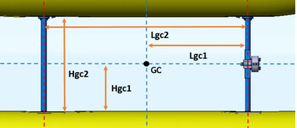
3.6 Definition of the geometric center (GC) (not to scale). . . 42

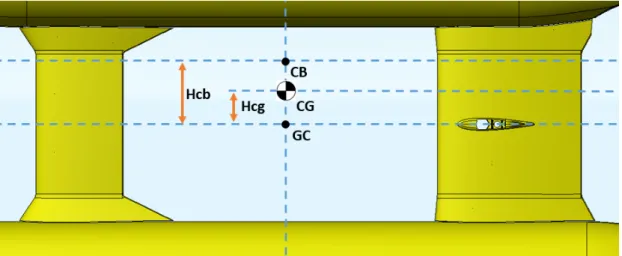
3.7 Location of geometric center (GC), CG, CB (not to scale). . . 43

3.8 Body-fixed axis for considered vehicle (not to scale). . . 43

3.9 Isometric view of the main structure. . . 46

3.10 Static damping forces as a result of motion in surge. . . 55

3.11 Static damping moments as a result of motion in surge. . . 56

3.12 Static damping forces as a result of motion in sway. . . 58

3.13 Static damping moments as a result of motion in sway. . . 58

3.14 Static damping forces as a result of motion in heave. . . 59

3.15 Static damping moments as a result of motion in heave. . . 60

4.1 Longitudinal subsystem trajectory for the dive and ascent maneuver (80s simula-tion). . . 69

4.2 Longitudinal subsystem AoA and pitch angle for the dive and ascent maneuver (80s simulation). . . 70

4.3 Complete model trajectory for the dive and ascent maneuver (80s simulation). . 70

4.4 Complete model AoA and pitch angle for the dive and ascent maneuver (80s sim-ulation). . . 71

4.5 Terminal velocity for the zig-zag maneuver. . . 72

4.6 Lateral subsystem trajectory for the zig-zag maneuver (80s simulation). . . 73

4.7 Lateral subsystem side-slip, yaw and roll angles for the zig-zag maneuver (80s simulation). . . 73

4.8 Complete model trajectory for the zig-zag maneuver (80s simulation). . . 74

4.9 Complete model attitude, AoA and side-slip angles for the zig-zag maneuver (80s simulation). . . 74

4.10 Helical diving test trajectory (Color bar indicates time - 80s). . . 76

4.11 Helical diving test attitude, AoA and side-slip angle (80s simulation). . . 76

(14)

LIST OF FIGURES LIST OF FIGURES

A.1 Lateral subsystem velocities for the zig-zag maneuver (80s simulation). . . 89 A.2 Complete model velocities for the zig-zag maneuver (80s simulation). . . 90 A.3 Longitudinal subsystem velocities for the dive and ascent maneuver (80s simulation). 91 A.4 Complete model velocities for the dive and ascent maneuver (80s simulation). . . 91

(15)

LIST OF TABLES LIST OF TABLES

List of Tables

1.1 Translation DoFs. . . 9

1.2 Rotational DoFs. . . 10

3.1 Dimensions for figures 3.2, 3.3, 3.4 and 3.5 (in millimeters). . . 41

3.2 Distances for figure 3.6 (in millimeters). . . 42

3.3 Distances of 3.7 (in millimeters). . . 43

3.4 Mass [kg] and Inertia [kg· m2_{] for this vehicle. . . .} ₄₆

3.5 Distance parameter for upper body. . . 53

3.6 Distance parameter for lower body. . . 53

3.7 Parameters for added mass estimation of the upper body. . . 53

3.8 Parameters for added mass estimation of the lower body. . . 53

3.9 Total added mass estimation for the upper body. . . 54

3.10 Total added mass estimation for the lower body. . . 54

3.11 Linear damping coefficients for motion in surge. . . 56

3.12 Quadratic damping coefficients for motion in surge. . . 56

3.13 Linear damping coefficients for motion in sway. . . 59

3.14 Quadratic damping coefficients for motion in sway. . . 59

3.15 Linear damping coefficients for motion in heave. . . 60

3.16 Quadratic damping coefficients for motion in heave. . . 60

4.1 Vertical thrust for the dive and ascent maneuver. . . 69

4.2 Motor thrust for zig-zag maneuver. . . 72

(16)

(17)

LIST OF TABLES LIST OF TABLES

List of Acronyms

2D Two Dimensions

3D Three Dimensions

AUV Autonomous Underwater Vehicle

CAD Computer-Aided Design

CB Center of Buoyancy

CEiiA Centro de Engenharia e Desenvolvimento de Produto

CFD Computational Fluid Dynamics

CG Center of Gravity

DNV GL Det Norske Veritas Germanischer Lloyd

DoF Degree of Freedom

DVL Doppler Velocity Log

NED North-East-Down

ECEF Earth-Centered Earth-Fixed

GC Geometric Center

GPS Global Positioning System

INS Inertial navigation system

LBC Lower Body Center

NDD Nominal Diving Depth

PID Proportional–Integral–Derivative

ROV Remotely Operated Vehicle

SNAME Society of Naval Architects and Marine Engineers

UBI University of Beira Interior (EN)

UBL Upper Body Center

US United States

(18)

(19)

Chapter 1 • Introduction

Chapter 1

Introduction

The ocean has been a source of valuable resources throughout human history. Although humans have ”sailed the seven seas” and actively exploited this mean for resources, our knowledge of the underwater environment remains limited. Extreme pressures, high corrosion, low visibility, limitations in underwater communications, difficult access and unstable environmental condi-tions are few reasons that make the ocean a difficult medium to explore. Ever since the first ships sailed towards the unknown that these challenges are a source of great mythical fears, as found in popular literature like Os Lusíadas by portuguese poet Luís de Camões. Nowadays, superstition has given place to science, but the challenges for marine exploration remain. Remotely Operated Vehicles (ROVs) have been the workhorse of underwater exploration. ROVs maintain communication and receive power via a umbilical-tether between the vehicle and a dedicated support vessel. A skilled operator is often required to control the craft. The need for a dedicated support vessel and a skilled operator translates into high operational costs. Recently, modern technology, most notably in computer science, allowed the advent of the Autonomous Underwater Vehicle (AUV). AUVs, like ROVs, are a type of Unmaned Underwater Vehicle (UUV)1_{. The AUV operates autonomously, meaning that the AUV’s mission has to be}

pre-programmed before its deployment. Since no physical link is present between the vehicle and the support vessel, the risk of vehicle loss is substantial, thus, assuring survivability is a complex, multi-variable task. The independence of AUV is, at the same time, the greatest advantage and disadvantage of these systems.

Presently, ocean exploration is a subject of great interest for military, economic and scientific purposes. These are the main sources of applications for AUVs. Versatility and independence makes the AUV a useful tool capable of addressing current needs. Either for cost reduction or increased capability, the interest for the technology certainly exists [2, 3]. The military sector was the first to experiment with AUVs, during the 1960’s. Sumbarine launched nuclear ballistic missiles is one, probably the most worrying, of many marine threats in the case of war. The AUV can be used to conteract such threats and provide unprecedented millitary capability [4]. Today, the millitary sector is still the most significant client in the AUV market. Academic organizations also started developing AUVs aimed for specific scientific studies. In the last decade, the use of AUVs to collect data led to major advances in oceanography. Such studies allow humans to obtain valuable knowledge about the natural laws and forces that govern our oceans [5]. The use of AUVs remained limited to the public sector until the oil & gas industry showed interest in the technology for cost reduction purposes. After sucessfull experiments with AUVs this industry became the first major commercial application of AUVs. Offshore hydrocarbon exploration is already well established: the number of offshore oil rigs is just below 500 and rising [6].

1

The class organization of ROV, UUV and AUV may differ depending on the author. The adopted class organization is devised from DNV GL [1].

(20)

Chapter 1 • Introduction

The mission of an AUV is dependent on its purpose. Although some mission scenarios are common for these vehicles, such as mapping and reconnaissance, it makes sense to organize character-istic applications in terms of purpose:

• Military applications - These range from intelligence, surveillance and reconnaissance to expeditionary and anti-submarine warfare and mine disposal. In The Navy Unmanned

Undersea Vehicle (UUV) Master Plan [4] one can find more information about the US Navy’s

strategy to develop new and extend on current AUV capabilities.

• Commercial applications - Inspection, either for environmental or engineering purposes, of pipelines, communication lines and underwater structures are the primary commercial application of AUV’s. [6, 7]. Other emerging applications include mapping and identifica-tion of underwater mineral deposits and inspecidentifica-tion of aquaculture sites.

• Research applications - According to Wynn et al., 2014 [5] four main applications are devised that can be adapted to: habitat mapping in deep- and shallow-water; study of volcanic and hydrothermal vents; temperature monitoring; and mapping of ocean terrain. These sectors are currently responsible for approximately 50%, 20% and 30%, respectively, of the AUV market (estimated 200 million (US$) in 2012). By contrast, the ROV market represented an estimated value of 850 million (US$) in the same period [2]2_{. This discrepance can be credited}

to the high degree of maturaty of the ROV technology and limitations inherent to the nature of AUVs. Although autonomy, communications, navigation, data storage and short life cycles present complex challenges that limit the use of AUVs [3], these do not seem to compromise the use of AUVs for future missions since the AUV market is estimated to reach 2.3 billion (US$) by 2019 [2]. Furthermore, integration of marine technologies such as ROVs, AUVs, towed underwater vehicles and unmanned surface vehicles is an active field of research that may prove valuable.

(21)

Historical Overview of UUV’s and Control Theory Chapter 1 • Introduction

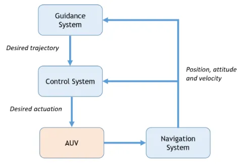
The autonomous nature of AUVs imply a high level of reboutness of the guidance, navigation

and control system(s). One of the most challenging limitations for navigation is underwater

communication: the high electrical conductivity of water inhibits the use of electromagnetic positioning (such as GPS3_{) and communication systems. The best available option is accustic}

systems, however, short range and low transfer rates restric its use for positioning and high data flux communication [3]. AUV navigation is therefore traditionally achieved by inertial navigation

systems (INS) [8]. The data from the navigation system is relayed to the guidance system, this

system is responsible for computing the desired motion that the vehicle should follow to achieve a given trajectory. A reference model is traditionally used to assure feasible trajectories. The control system can then determine the necessary forces and moments that should be imposed on the vehicle to achieve the desired motion. This forces and moments are imposed using the control actuators i.e. thrusters and control surfaces, if present [9].

1.1 Historical Overview of UUV’s and Control Theory

The first vehicle that can be classified as an UUV is the Whitehead self-propelled torpedo, developed during the 1860’s by Robert Whitehead [10, 11]. This vehicle can also be classified as the first AUV since it operated autonomously. Early torpedos operated using a Pendulum-and-hydrostat for depth-keeping and a gyroscopic steering system for course-keeping [11].

The early 20th_{century marked the beginning and subsequent expansion of feedback controllers}

(see figure 1.2) for a number of applications, most notably, the PID (Proportional–Integral– Derivative) controller was first introduced on ships for automatic steering [12]. Although, simple control systems were being implemented, limitations of current methods and little understand-ing of the underlyunderstand-ing mathematical principles in control meant that only so much could be achieved and most applications were based on a trial and error approach [13].

Figure 1.2: A block diagram of a negative feedback control system.

The development of unmanned submersibles remained limited to the torpedo until 1953 when the first ROV, nicknamed ”poodle”, was developed by Dimitri Rebikoff [14]. In control theory, the 1950’s witnessed the advent of modern control: the popularization of the state-space approach, by engineers working in the aerospace industry, meant that complex physical models could be used for the design of feedback controllers. This new approach also facilitated the use of existing

3

(22)

Chapter 1 • Introduction Classification and Norms

tools of analysis for differential equations (e.g Lyapunov stability) and allowed for new concepts such as observability and controllability by Kalman [12, 13].

The initial development of AUV’s started in the early 1960’s and by the late 1960’s, AUV’s were used for military, research and oceanographic purposes. During the 1970’s the discovery of oil in the North sea prompted the development of unmanned submersibles, mainly ROV’s, capable of deep sea exploration and tasks associated with hydrocarbon exploration [6]. However, It was not until the 1980’s and early 1990’s that major leaps in computer technology allowed for small, powerful and reliable motion control. This technology allowed for a ”boom” in AUV related research followed by routine commercial operations during the 2000’s [15, 6, 16, 17, 18]. As the AUV technology matures, commercial and noncommercial markets are expected to grow [3].

1.2 Classification and Norms

AUV’s are now classified as underwater robots (robot (as in Encyclopaedia Britannica [19]) - any automatically operated machine that replaces human effort, though it may not resemble human beings in appearance or perform functions in a human-like manner).

In auvac.org [20], a website dedicated to collect and share information about AUV systems, AUV’s are differentiated in terms of purpose, body type and class. Up to twenty different pur-poses are devised for military applications, commercial use and scientific investigation. Eleven body types and four classes are discern. In The Navy Unmanned Undersea Vehicle (UUV) Master

Plan [4] AUV’s are organized by displacement and diameter. For the purpose of this thesis,

displacement and body type are enough for classification.

1. Man-Portable class – Vehicle displacement from 10 kg to 50 kg. 2. Light Weight Vehicle class – Vehicle displacement of about 250 kg. 3. Heavy Weight Vehicle class – Vehicle displacement of about 1 400 kg. 4. Large Vehicle class – Vehicle displacement of about 10 000 kg.

This classification is far from proper and should be taken accordingly. However, it may serve as a precursor for a more significant classification.

A simple way to classify body types is by the number of hulls: single or multi. Most AUVs follow the single hull (or single body) configuration, with special emphasis on the torpedo shape. Probably the greatest advantage of such systems is in hydrodynamic efficiency due to ther lower contact area with the surrounding fluid. Multi-hull AUVs are typically comprised of two or three hulls. The Multi-hull configuration allows for greater flexibility in the distribution of of weight and buoyant force. Allocating heavy components to the lower body allows for the center of

(23)

The AUV Chapter 1 • Introduction

refered to as the metacentric height, the more stable the vehicle. This could be significant when considering missions that require the vehicle to be as stable as possible e.g. mapping [21]. On the downside, drag forces and weight are typically greater for multiple body AUVs. When designing a new product, the use of norms, ideally standards, in all stages of the project is of major importance. These help assure product feasibility. Although no standards exist for the control of AUVs, norms from Det Norske Veritas Germanischer Lloyd (DNV GL) are available [1]. The design of this AUV tries to comply with the norms from DNV GL.

1.3 The AUV

Figure 1.3: 3D model of the AUV being developed at CEiiA (courtesy of CEiiA).

The AUV being developed at CEiiA (see figure 1.3) is a double body, light weight research AUV capable of a Nominal Diving Depth (NDD)4 _{of 3,000 meter.}

The vehicle is comprised of two pressure hulls. The lower pressure hull houses the batteries and the upper one houses all necessary systems and sensors, as well as data storage equipment. The weight force is counteracted by adding low density syntactic foam which provides extra buoyancy. In order to increase the metacentric height, most syntactic foam is located in the upper body.

4

Nominal Diving Depth - The maximum diving depth for unrestricted operation of an underwater vehicle (In accordance with [1]).

(24)

Chapter 1 • Introduction The AUV

This AUV carries a variety of sensors for data acquisition and navigation. The sensors used for underwater navigation include:

• Inertial Navigation System (INS) - Comprised of accelerometers and gyroscopes. By in-tegrating linear and angular accelerations this system allows estimation of position and velocity. The gyroscope determines the orientation.

• Magnetometer - Using electromagnets, the magnetometer determines the magnetic north by analyzing the disturbance in the electromagnet’s magnetic field caused by the Earth’s magnetic field.

• Doppler Velocity Log (DVL) - This equipment uses the acoustic Doppler principle to estimate velocity. It may or may not include ocean current estimation.

• Underwater Altimeter - The altitude is estimated by sending an acoustic signal towards the seabed. Knowing the velocity of sound in water it is possible to calculate the distance. The propulsive system is comprised of four identical thrusters, two vertical and two horizontal. The vertical thrusters are embedded in the hulls: the forward engine in the lower body and the aft engine in the upper body. The position of the longitudinal thrusters can be seen in section 1.3. These provide the necessary force to propel the vehicle forward and, by applying a different force to each engine, allow the vehicle to change course.

An important feature of this vehicle is that the vertical and horizontal hydrodynamic fairings are designed to act as stabilizing surfaces. Considering that the vehicle is moving forward, the fairings induce lift forces that create a correcting moment. This is intended at keeping the vehicle parallel to the direction of the flow. The influence of the stabilizing surfaces in the general dynamics of the vehicle is addressed in section 3.2.5.

1.3.1 Mission

The AUV being developed at CEiiA follows the traditional research AUV mission, which can be divided into three main stages:

• Dive - Since ballast tanks are not present in this AUV, extra mass is carried in the bow to increase the weight force thus facilitating the descend. A spiral trajectory is to be performed through the water column with a nose down attitude (see figure 1.4). When mission depth is reached, this extra mass is released and residual buoyancy is achieved (see section 3.2.3).

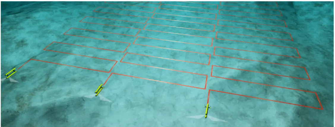
• Data acquisition - The typical sensor suit of research AUVs requires the vehicle to be capable of stable longitudinal ”flight” (small angles of attitude). The vehicle should be able of course keeping, changes in course and depth. A da aquisition scenario is performed

(25)

The AUV Chapter 1 • Introduction

Figure 1.4: Diving and ascending scenario (courtesy of CEiiA).

Figure 1.5: Mission scenario (courtesy of CEiiA).

• Ascent - Extra mass is also carried in the stern of the vehicle. When the mission is concluded the mass is released and buoyant forces overcome gravitational forces thus forcing the vehicle into a nose down ascent. Also to be preformed in a spiral manner (see figure 1.4).

1.3.2 Similar Vehicles

Although there are plenty of light weight AUVs, most are single body. Possibly the first successful double body, where both hulls are aligned vertically, AUV is the SeaBed thus, this configuration is sometimes referred as twin body type SeaBed.

(26)

Chapter 1 • Introduction The AUV

• Woods Hole Oceanographic Institution’s SeaBed

Figure 1.6: The Woods Hole Oceanographic Institution’s SeaBed AUV (adapted from [22]).

The SeaBed platform (figure 1.6), available in various configurations, has participated in a number of research missions, being currently operated by multiple institutions around the world. The standard SeaBed platform has a mass of 250 kg, a length of 2.5 m, maximum diving depth of 2,000 m and an endurance of approximately 8 hours. The success of the SeaBed led to the development of the Puma and Jaguar which improved capabilities of their predecessor [22]. The SeaBed validated the concept of a twin, vertical aligned hull AUV.

• Marport’s SQX-500

Figure 1.7: The Marport’s SQX-500 UUV (adapted from [23]).

The Marport’s SQX-500 is a more recent platform directed at military applications. The vehicle presents a mass of 95 kg, maximum diving depth of 500 meter, it is 1.6 meters long, has 8 hours of endurance and a cruise speed of 2 m/s. This vehicle is capable of moving its vertical rudders 180◦in all directions, providing the SQX-500 with great maneuverability.

(27)

Terminology Chapter 1 • Introduction

1.4 Terminology

”Nomenclature for Treating the Motion of a Submerged Body Through a Fluid” is the title of a

1950 report by the American Society of Naval Architects and Marine Engineers (SNAME) [24] that aimed to normalize nomenclature and notation in this field. This, or a similar version of it, is the most common nomenclature and notation used today when treating underwater vehicles, it is therefore used as reference for this thesis and will be address as SNAME notation hereinafter. Moreover, in recent years, Fossen’s Guidance and Control of Ocean Vehicles [25] became a common reference for modeling purposes. In Guidance and Control of Ocean Vehicles, Fossen expands the SNAME notation to address certain particularities. Notation and arrangements in this reference are also adopted.

1.4.1 Motion

Underwater vehicles experience motion in 6 Degrees of Freedom (DoF), i.e. complete freedom of movement. Two categories can be devised when considering the nature of motion, 3DoF for translation and 3DoF for rotation. According to SNAME notation:

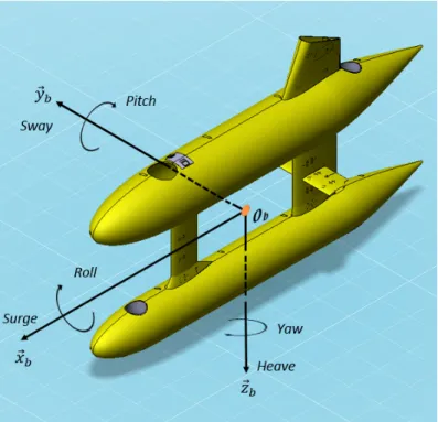
Figure 1.8: Motion variables for the body-fixed reference frame i.e.{b} = (xb, yb, zb)

.

Table 1.1: Translation DoFs.

Terminology Motion along Position Velocity Force

Surge xb x u X

Sway yb y v Y

(28)

Chapter 1 • Introduction Terminology Table 1.2: Rotational DoFs.

Terminology Rotation about Attitude Angular velocity Moment

Roll xb ϕ p K

Pitch yb θ q M

Yaw zb ψ r N

Tables 1.1 and 1.2 presents terminology and notation for translation and rotation, respectively. Figure 1.8 summarizes motion for 6DoF.

1.4.2 Vector Notation for 6DoF

It is useful to express dynamic properties in vectorial notation for purposes of simplicity and organization. The adopted notation is now produced in the context of expressing motion in 6DoF. This includes organizing vectors by qualitative property and expressing them in terms of reference frames. Two types of reference frames are of interest for the purpose of this thesis: a local North-East-Down (NED) {n} reference frame, which is inertial, and the body-fixed {b} reference frame (see section 1.6.1.1).

Arrangement: The argument represents the physical property, the superscript represents the

frame where this property is expressed, the subscript represents the point of action (if in frac-tion, the denominator denotes the reference point).

Example: pe

b n

= Position of point 0b (origin of {b}) with respect to {n}, expressed in {e}

reference frame. • Position vector pn b n =    N E D    ∈ R3

The position vector expresses the vehicle’s position in 3D space in{n} (see section 1.6.1.1). • Attitude vector Θnb=    ϕ θ ψ    ∈ S3 _{q =}       q0 q1 q2 q3      ∈ R 4

• Linear velocity vector υb

b n =      u v w     ∈ R3

(29)

Overview of Dynamic Models for Underwater Vehicles Chapter 1 • Introduction

• Angular velocity vector ωbb n =      p q r     ∈ R3 • Force vector fb_b=      X Y Z     ∈ R3 • Moment vector mb b=      K M N     ∈ R3

The complete vector representation for 6DoF can be expressed by the following vectors:

• Position and attitude vector η =

 pnb n q   ∈ R7 _; _{η =}  pnb n Θnb   ∈ R3_{× S}3

• Velocity and acceleration vector ν =

 υbb n ωb b n   ∈ R6

• Force and moment vector τ =

 fbb mb b   ∈ R6

1.5 Overview of Dynamic Models for Underwater Vehicles

The post Second World War period saw the advent of the state-space approach. Simply put, the method involves modeling a system (or plant), such as an AUV, by creating a mathematical model which is represented by first-order differential equations. The controller is design to satisfy model particularities. In the context of this thesis, the dynamic model is the set of first order differential equations that describe the vehicle’s motion. Simulation of the dynamic model is achieved by solving this equations by integration [26].

The standard equations of motion for submarines were published in 1967 by Gertler, at the request of the US Navy and can be found in [27]. These equations were subsequently revised in 1979 by Feldman [28]. The standard equations of motion for submarines are highly accurate due to the extent to which the hydrodynamic coefficients are addressed [29]. The intrinsic nature of manned submarines introduces the need for such accurate models and the state-of-art in hydrodynamic modeling, most notably in terms of test facilities and man-power. The costs associated with the development of AUVs do not compare to those of a manned submarine

(30)

Chapter 1 • Introduction Overview of Dynamic Models for Underwater Vehicles

[30]. On the other hand, unlike submarines, AUVs operate autonomously so robust and accurate control is paramount. In this context, it is of the utmost importance to evaluate requirements and capacity in order to choose the appropriate modeling approach.

Some of the most important considerations are summarized below:

• The mission (discussed in section 1.3) does not require extreme maneuvering capability. • High speed is not required.

• No experimental tests are possible at the time.

• Since control is the main purpose, applicability of modern control methods is important. In the context of these considerations it is clear that the standard equations of motion for submarines are not the answer since very detailed hydrodynamic characterization is not pos-sible. However, other, less complex options are available. In Modeling and simulation of the

autonomous underwater vehicle, Autolycus [30], Tang compares the most popular ethods for

modeling AUVs: Humphrey’s, Nahon’s and Fossen’s models.

• Humphrey’s model - Humphrey [31] used symmetry and other simplifications to linearize the equations of motion and decouple the longitudinal and lateral motion. The transfer functions are also provided for simpler implementation. However, no methods are provided to estimate hydrodynamic coefficients.

• Nahon’s model - This model follows a different approach to that of Humphrey’s. Instead of linearizing the model, Nahon searched for methods to estimate coefficients solely by the vehicle’s geometry, using both computational and analytical methods for the effect, while retaining the nonlinear nature of the equations of motion [32].

• Fossen’s model - Undoubtedly the most used method in modern literature, this model shares characteristics with the latter, the great advantage is that the equations of motion are arranged to facilitate the use o nonlinear control tools [29]. The model is a set of nonlinear equations arranged in matrix form and simple methods to estimate hydrodynamic coefficients are provided to a certain extent [33].

(31)

Fossen’s Model for Marine Craft Chapter 1 • Introduction

Since it is a proven method and satisfies the considerations discussed in this section, Fossen’s model is used for modeling the AUV being developed at CEiiA. Fossen’s model can be expressed in accordance with Fossen’s Nonlinear Modelling and Control of Underwater Vehicles [33].

˙

η = J (η)ν (1.1)

M ˙ν + C(ν)ν + D(ν)ν + g(η) = τ (1.2)

Equation 1.1 represents kinematics and equation 1.2 represents kinetics (see section 1.6). Where J is a vector transformation matrix. M , C and D denote the mass, Coriolis and Damp-ing, respectively, g(η) represents the hydrostatic forces and τ is the applied external forces vector.

1.6 Fossen’s Model for Marine Craft

Dynamics can be divided into two branches of classic mechanics: kinematics and kinetics. The geometric aspects of motion are addressed in kinematics. This includes attitude, position, velocity, acceleration and subsequent concepts such as trajectory, rotation, reference frames, etc. In turn, kinetics is the study of internal and external forces and moments that dictate the dynamic characteristics of a given vehicle.

1.6.1 Kinematics

This section addresses the different aspects of kinematics. A brief description of the used reference frames in the context of Galilean relativity is produced. Navigation angles are sub-sequently presented and the problematic of vector transformation between reference frames is also addressed.

1.6.1.1 Reference Frames

Understanding reference frames is essential when modeling vehicles considering that our main concern is motion, and motion is relative to some reference. For navigation in large areas, the earth-centered, earth-fixed (ECEF) reference frame{e} = (xe, ye, ze)is used, yet, considering

(32)

Chapter 1 • Introduction Fossen’s Model for Marine Craft

and longitude are small, a local reference frame can be adopted. In this context, two reference frames are selected to express and simulate motion. The body-fixed and a local NED reference frames [9]. These Cartesian frames follow the right hand rule.

• Local NED{n} = (xn, yn, zn)– An inertial reference frame that represents a tangent plane

normal to a fixed point 0n (the reference frame’s origin), in the earth’s surface. The{n}

vector components are respective representations of north, east and down coordinates. • Body-fixed{b} = (xb, yb, zb)– A non-inertial reference frame that is coupled to the body.

This frame exhibits rotation and acceleration relative to the Earth-fixed inertial reference frame. The {b} vector components represent, respectively, the longitudinal, transverse and normal axes of the vehicle (see figure 1.8). The origin is expressed as 0b.

Considerations of the Body-fixed reference frame The center of the Body-fixed reference frame {b} is usually appointed, either to coincide with the center of gravity (CG) or in some geometrically meaningful location, since this locations are typically well defined and less likely to suffer modification e.g. location symmetry planes intersection, geometrical midpoints, etc. Two important point to consider when designing an underwater vehicle are the CG and the CB.

rbg=

[

xg yg zg

]T

denotes the position vector for CG with respect to 0b.

rb B =

[

xB yB zB

]T

denotes the position vector for CB with respect to 0b.

1.6.1.2 Navigation angles

Flow related angles When a vehicle travels through a fluid, the incidence of the flow relative to the body axes i.e. the velocity vector is of great importance because the hydrodynamic forces are perpendicular (drag) and parallel (lift) to the flow. This suggests that another, ”flow oriented”, reference frame can be devised. This frame is commonly referred as flow axes ({f} = (xf, yf, zf)). The origin of{s} frame is the same as the {b} frame.

The angle between xband the projection of xf in the xbzbplane is denoted angle of attack (AoA

or α).

(33)

Although flow axes can be useful for hydrodynamic analysis, a perhaps simpler way to determine the angle of attack and the side-slip angle is by analyzing the velocity vector υb

b n

. The magnitude of the velocity vector is expressed by:

U =√u2_{+ v}2_{+ w}2 _(1.3)

Figure 1.9: Definition of angle of attack and side-slip, respectively (adapted from [34]).

From figure 1.9,and in accordance with [34], the following relation between velocity and these angles can be devised.

α = tan−1(w

u) (1.4) β = sin−1(v

U) (1.5)

Orientation related angles When navigating, whether for aircraft or marine craft, north is used as the orientation of reference, expressed in compasses as zero degrees. Following the NED Cartesian system and right hand rule, 90º points towards East, 180º towards South and 270º towards West. The angle between the projection of xbin the xbybplane and xndefines heading

(ϕ). If a side-slip angle is present, heading is not the direction of travel, the direction of travel is then denominated course (χ) and it is defined as the the sum of the side-slip angle and heading angle:

χ = β + ϕ. (1.6)

1.6.1.3 Transformation between Reference Frames

The underlying problem in transforming vectors between reference frames whose axes are not aligned is rotation. A handful of methods can be used to achieve vector rotation, but the two

(34)

most common methods are Euler angles and quaternions. Transformation using quaternions is significantly faster, in terms of computation, and singularities are avoid. However, Euler angles are more intuitive [35],[36], [37],[38]. Both quaternions and Euler angles were used for the 6DoF model (see chapter 4). For the purpose of data presentation and to devise the longitudinal and lateral subsystems (see chapter 2), Euler angles were used.

Quaternion Quaternions are a 4th _{order complex number system introduced by William R.}

Hamilton in 1843 and present similar properties to complex numbers. When considering the imaginary and real parts of a complex number as coordinate axis of the Cartesian plane, an association can be devised and used to translate and rotate a point and hence to transform a vector. However, for a 3D geometry, 4th_{order complex numbers are necessary to obtain similar}

capacities [39].

A quaternion q can be expressed as:

q = qo+ q1i + q2j + q3k (1.7)

Note that:

i2_{= j}2_{= k}2_{= ijk =}₋₁

Expressed in vector form:

q = [ q0 ε ]T ∈ R Where, ε =      q1 q2 q3     ∈ R3

1.6.1.4 Linear Velocity Transformation

Transformation is attained by means of multiplying the body’s velocity vector by a rotation

matrix Rf rom_to .

For quaternions linear velocity transformation can be expressed like:

˙

(35)

Fossen’s Model for Marine Craft Chapter 1 • Introduction Where: Rn_b(q) =      1− 2(q2₂+ q₃2) 2(q1q2− q3q0) 2(q1q3+ q2q0) 2(q1q2+ q3q0) 1− 2(q21+ q23) 2(q2q3+ q1q0) 2(q1q3+ q2q0) 2(q2q3+ q1q0) 1− 2(q21+ q22)     

And for Euler angles:

˙ pn_b/n= Rnb(Θnb)υ b b/n (1.9) Where: Rn_b(Θnb) =     

cos(ψ) cos(θ) − sin(ψ) cos(ϕ) + cos(ψ) sin(θ) sin(ϕ) sin(ψ) sin(ϕ) + cos(ψ) sin(θ) cos(ϕ) sin(ψ) cos(θ) cos(ψ) cos(θ) + sin(ϕ) sin(θ) sin(ψ) − cos(ψ) sin(ϕ) + sin(θ) sin(ψ) cos(θ)

− sin(θ) cos(θ) sin(ϕ) cos(θ) cos(ϕ)

     Note that (Rn b)−1= (R n b) T_.

Angular Velocity Transformation Transformation is attained by means of multiplying the vec-tor of interest by a transformation matrix T.

For quaternions: ˙ q = Tq(q)ωbb/n (1.10) Where: Tq(q) =         −q1 −q2 −q3 q0 −q3 q2 q3 q0 −q1 −q2 q1 q0        

For Euler angles:

˙

(36)

Chapter 1 • Introduction Fossen’s Model for Marine Craft Where: TΘ(Θnb) =     

1 sin(ϕ) tan(θ) cos(ϕ) tan(θ)

0 cos(ϕ) − sin(ϕ)

0 sin(ϕ)/ cos(θ) cos(ϕ)/ cos(θ)      1.6.1.5 Kinematics Equation Since η =  pnb n q 

, the kinematics equation for an AUV moving in the {n} reference frame is expressed as: ˙ η = J (η)ν (1.12) • If using quaternions: ˙ η = Jq(η)ν (1.13)

Equation 1.13 expands to:

 p˙nb n ˙ q   =  Rnb(q) 03_×3 03_×3 T(q)   ·  υbb n ωb b n  

• If using Euler angles:

˙

η = JΘ(η)ν (1.14)

Equation 1.14 expands to:

 p˙nb n ˙ Θnb   =  Rnb(Θnb) 03×3 03×3 T(Θnb)   ·  υbb n ωb  

(37)

1.6.2 Kinetics

Kinetics, as previously stated, addresses the relationship between motion and force. An under-water vehicle is exposed to the same laws of motion that govern all bodies, under the assumption that the vehicle can be considered rigid, these laws are traditionally referred to as the equations of motion for a rigid body. Since the surrounding fluid is water, a variety of hydrostatic and hydrodynamic forces are also present. The influence of these forces is mostly dependent on the geometry and mass of the vehicle. Estimation of parameters of interest presents a complex task which is addressed in chapter 3. For the purpose of this thesis, three assumptions are devised from an early stage in the project:

• Low operational velocities.

• Ocean currents are unaccounted for.

• Operating area is large enough for unrestricted motion. Other vehicle-specific constrains are expressed in section 3.2.1.

1.6.2.1 Rigid-Body Equations of motion

The relationship between motion and force in the context of classical mechanics was introduced by Isaac Newton in Philosophiæ Naturalis Principia Mathematica Newton’s Three Laws of Motion [40]. Considering the vehicle is rigid, the 6DoF rigid-body equations of motion can be expressed, in matrix form, as:

Mrb· ˙ν + Crb(ν)· ν (1.15)

Where Mrb is the rigid body mass matrix and Crb represents the rigid body Coriolis forces

matrix. The rigid body mass matrix is expressed according to Fossen, 2011 [9]:

Mrb=  m· I3_×3 −S(rbg) m· S(rb g) Ib   (1.16)

(38)

Where m is the mass of the vehicle, I3_×3is a 3× 3 identity matrix, S(rbg)is the skew-symmetric

matrix5 _{of r}b

gand Ibis the vehicle’s inertia tensor. This expands to:

Mrb=               m 0 0 0 m· zg −m · yg 0 m 0 −m · zg 0 m· xg 0 0 m m· yg −m · xg 0 0 −m · zg m· yg Ix −Ixy −Ixz m· zg 0 −m · xg −Iyx Iy −Iyz −m · yg m· xg 0 −Izx −Izy Iz               (1.17)

When an object’s movement is expressed in terms of a non inertial reference frame, in this case the Body-fixed reference frame, additional forces seem to appear, the Coriolis and centrifugal forces [9].

The Coriolis and centrifugal forces matrix can be expressed according to Fossen and Fjellstad, 2005 [35]. Crb(ν) =   03×3 −m · S(ν1)− m · S(ν2)· S(rbg) −m · S(ν1) + m· S(rbg)· S(ν2) −S(Ibν2)   (1.18) =               0 0 0 m(ygq + zgr) −m(xgq− w) −m(xgr + v) 0 0 0 −m(ygp + w) m(zgr + xgp) −m(ygr− u) 0 0 0 −m(zgp− v) −m(zgq + u) m(xgp + ygq)

−m(ygq + zgr) m(ygp + w) m(zgp− v) 0 −Iyzq− Ixzp + Izr Iyzr + Ixyp− Iyq

m(xgq− w) −m(zgr + xgp) m(zgq + u) Iyzq + Ixzp− Izr 0 −Ixzr− Ixyq + Ixp m(xgr + v) m(ygr− u) −m(xgp + ygq) −Iyzr− Ixyp + Iyq Ixzr + Ixyq− Ixp 0              

(39)

1.6.2.2 Hydrostatics

In hydrostatics, two forces are considered: buoyancy and gravitational forces.

Archimedes’ principle - A body immersed in a fluid is subjected to an upwards force equal to

the weight of the displaced fluid [41]. This force is designated as buoyancy force.

B = ρg∇ (1.19)

Where ρ is the density of the fluid, g is the acceleration of gravity and ∇ is the volume of fluid displaced by the vehicle. The buoyancy force acts upon CB, parallel to zn, in the negative

direction. Expressed in{n}: fn_B=      0 0 −B      (1.20)

The gravitational force (or weight) is derived from Newton’s 2nd_{Law of motion.}

W = mg (1.21)

Where m is the mass and g is the acceleration of gravity. The gravitational force acts upon the CG, parallel to zn, in the positive direction. Expressed in{n}:

fn_g =      0 0 W      (1.22) Expressed in{b}: fb_B= Rn_b(q)−1fn_B (1.23) fb_g= Rn_b(q)−1fn_g (1.24)

(40)

The resulting forces and moments are referred to as restoring forces. The restoring forces vector g(η) can be expressed as:

g(η) =−   fbB+ f b g rb Bf b B+ rbgf b g   (1.25)

If using Euler angles, this expands to:

g(η) =               (W− B) sin(θ) −(W − B) cos(θ) sin(ϕ) −(W − B) cos(θ) cos(ϕ)

−(ygW − yBB) cos(θ) cos(ϕ) + (zgW− zBB) cos(θ) sin(ϕ)

(zgW− zBB) sin(θ) + (xgW− xBB) cos(θ) cos(ϕ)

−(xgW − xBB) cos(θ) sin(ϕ)− (ygW− yBB) sin(θ)

              (1.26)

1.6.2.3 Hydrodynamic Added Mass

When a vehicle accelerates through a fluid a phenomena occurs in which some of the vehicles kinetic energy is transferred to the fluid due to friction, this results in extra resistance to ac-celerations. If the fluid density is much lower than the vehicle’s e.g. air, this effect can be neglected yet, if those are similar, the vehicle behaves as if it had more mass then it actually does. Hence, the phenomena is generally known as added mass. If the mean is water, one can address this phenomena as hydrodynamic added mass.

In [42], the complete expressions for added mass are produced for an ideal fluid.

The kinetic energy of the fluid surrounding the vehicle TAcan be expressed according to [42]:

TA=

1 2νMAν

(41)

Where MAis the added mass matrix:

MA=−               Xu˙ Xv˙ Xw˙ Xp˙ Xq˙ Xr˙ Yu˙ Yv˙ Yw˙ Yp˙ Yq˙ Yr˙ Zu˙ Zv˙ Zw˙ Zp˙ Zq˙ Zr˙ Ku˙ Kv˙ Kw˙ Kp˙ Kq˙ Kr˙ Mu˙ Mv˙ Mw˙ Mp˙ Mq˙ Mr˙ Nu˙ Nv˙ Nw˙ Np˙ Nq˙ Nr˙               (1.28)

As defined by SNAME [24], the upper half of the matrix elements represents the typical inertia coefficient i.e. the derivative of the force component with respect to an acceleration (linear or angular) component, e.g. Xu˙ = ∂X_{∂ ˙}_u. The lower half of the matrix elements represents the

typical moment of inertia coefficient i.e. the derivative of the moment component with respect to a acceleration component, e.g. Ku˙ = ∂K_{∂ ˙}_u.

Alternatively, this can be understood as the corresponding axial force or moment due to an acceleration.

Experimental methods are typicaly used to estimate hydrodynamic coeficients, however, an-alytical methods are also used to estimate added mass, either by specialized programs, like

WAMIT 6 _{or ESAM [43], or by simplifying the vehicle’s shape so that complex, time-consuming}

expressions can be avoided. Recently though, transient analysis in CFD has produced results in accordance with theoretical ones [44].

The Coriolis matrix due to added mass is expressed as:

CA(ν) =               0 0 0 0 −a3 a2 0 0 0 a3 0 −a1 0 0 0 −a2 a1 0 0 −a3 a2 0 −b3 b2 a3 0 −a1 b3 0 −b1 −a2 a1 0 −b2 b1 0               (1.29) 6 http://www.wamit.com/

(42)

Chapter 1 • Introduction Fossen’s Model for Marine Craft Where, a1= Xu˙u + Xv˙v + Xw˙w + Xp˙p + Xq˙q + Xr˙r a2= Yu˙u + Yv˙v + Yw˙w + Yp˙p + Yq˙q + Yr˙r a3= Zu˙u + Zv˙v + Zw˙w + Zp˙p + Zq˙q + Zr˙r b1= Ku˙u + Kv˙v + Kw˙w + Kp˙p + Kq˙q + Kr˙r b2= Mu˙u + Mv˙v + Mw˙w + Mp˙p + Mq˙q + Mr˙r b3= Nu˙u + Nv˙v + Nw˙w + Np˙p + Nq˙q + Nr˙r 1.6.2.4 Hydrodynamic Damping

Since the density of water is high when compared to other means where earth vehicles operate, drag forces are greater. Even at low speeds, like the ones experienced by most UUV, the drag component is considerable and should therefore be modeled correctly. More over, due to high fluid viscosity, this property should be taken into account.

The drag force can be modeled using the drag equation:

FD=−

1

2ρ CD A0V

2 _(1.30)

Where CDis the is the drag coefficient, A0represents the reference area and V is the velocity.

6DoF Damping for underwater vehicles can be described mathematically as:

Dn(ν)ν =               | ν |T _D n1ν | ν |T _D n2ν | ν |T _D n3ν | ν |T _D n4ν | ν |T _D n5ν | ν |T _D n6ν               (1.31)

(43)

The hydrodynamic damping i.e. drag, of an underwater vehicle can be highly coupled and nonlinear. If moving with low velocity, it is common to use quadratic approximation:

D(ν) = Dl+ Dq(ν) (1.32) Where: Dl=−               Xu Xv Xw Xp Xq Xr Yu Yv Yw Yp Yq Yr Zu Zv Zw Zp Zq Zr Ku Kv Kw Kp Kq Kr Mu Mv Mw Mp Mq Mr Nu Nv Nw Np Nq Nr               (1.33) Dq(ν) =−               Xu|u|| u | Xv|v|| v | Xw|w|| w | Xp|p|| p | Xq|q|| q | Xr|r|| r | Yu|u|| u | Yv|v|| v | Yw|w|| w | Yp|p| | p | Yq|q|| q | Yr|r|| r | Zu|u|| u | Zv|v|| v | Zw|w|| w | Zp|p|| p | Zq|q|| q | Zr|r|| r | Ku|u|| u | Kv|v|| v | Kw|w|| w | Kp|p| | p | Kq|q|| q | Kr|r|| r | Mu|u|| u | Mv|v|| v | Mw|w|| w | Mp|p|| p | Mq|q|| q | Mr|r|| r | Nu|u|| u | Nv|v|| v | Nw|w|| w | Np|p|| p | Nq|q|| q | Nr|r|| r |               (1.34)

As defined by [24], the upper half elements represent the typical static force derivative and the lower half represent the typical static moment derivative.

Drag forces are traditionally modeled using experimental methods. Analytical methods are too complex, except for simple shapes [45]. Alternatively, computational methods can and have been exploited to some extent (see references [46, 47]).

1.6.2.5 External Forces

The force that moves an AUV is typically provided by trolling motors. The external forces vector

τ (or thrust vector) relates the geometric and thrust characteristics of each motor with the resultant forces and moments.

(44)

Chapter 1 • Introduction Complete Dynamic Model

For vehicles controled by thrusters, the thrust vector can be expresses as in [48]:

τ = LU (1.35)

Where U is the force vector representing the thrust provided by each motor and L is the mapping matrix that relates motor thrust to resulting forces and moments. An example of a mapping matrix can also be found in [48].

1.7 Complete Dynamic Model

The complete dynamic model is the association of the kinematic and kinetic equations (equations 1.1 and 1.2, repectively). ˙ η = J (η)ν M ˙ν + C(ν)ν + D(ν)ν + g(η) = τ (1.36) Where: M = Mrb+ MA C = Crb+ CA (1.37)

The dynamic model can be conveniently arranged like in [49] since it is convenient to present the nonlinear model in the ˙x = f (x, t) form [50].

M ˙ν =−(C(ν)ν + D(ν))ν − g(η) + τ (1.38)

Since M−1M = I (this proves that the inverse of M−1exists):

˙

ν = M−1[−(C(ν) + D(ν))ν − g(η) + τ ] (1.39)

(45)

Purpose and Contribution Chapter 1 • Introduction

1.8 Purpose and Contribution

Control of AUVs is a complex challenge. This is mainly due to the variety of nonlinear hydrody-namic forces that these vehicles are subjected to. Moreover, since AUVs operate autonomously and carry a variety of very expensive equipment thus, the possibility of vehicle loss could prove costly and places extra requirements for the performance of the control system. Although modern feedback controllers are very capable, the underlying dynamic model, and therefore the validity of its parameters, can have an impact on controller performance. It is therefore paramount to devote the necessary effort for the estimation and validation of model parame-ters.

In this context, the purpose of this thesis is to devise the dynamic model of a AUV being de-veloped at CEiiA - Centro de Engenharia e Desenvolvimento de Produto. This work is aimed at increasing CEiiA’s capabilities in the field of control for underwater vehicles. The main goal of the model is the design of the control system, however, the same can be used for simula-tion, devising reference models for navigation and performance analysis during and after vehicle development [9, 16, 51].

Figure 1.10: Common uses for the dynamic model.

An overview of dynamic models commonly used for underwater vehicles suggests that Fossen’s dynamic model for marine craft is the most suited for modeling the AUV being developed at CEiiA. Since the main purpose is the application of control and, in the scope of providing different control design approaches, the appropriate lateral and longitudinal models are devised. These subsystems allow a) for a better understanding dynamic characteristics of the vehicle within the horizontal and vertical planes b) a simpler approach for controller design. Data estimation is achieved using analytic and computational methods. Data estimated via computational methods is provided by CEiiA and subsequently adapted to satisfy model parameters. Upon completion of the model parameters, simulation programs were devised. These programs are suited for controller design, analysis of the maneuverability and analysis of stability. The validity of the lateral and longitudinal models is also addressed using simulation.

(46)

Chapter 1 • Introduction Outline

1.9 Outline

This thesis is organized in the following manner:

• Chapter 1 contextualizes the research developed in this thesis by providing a brief histor-ical introduction, a description of the reference AUV, the necessary bibliographic review and other relevant topics.

• In chapter 2 the longitudinal and lateral models are devised to meet the particularities of the considered AUV. This was performed by decoupling the lateral and longitudinal motions.

• Chapter 3 addresses the estimation of model parameters for the AUV being developed at CEiiA using analytic and computational methods.

• Chapter 4 validates the lateral and longitudinal models by comparing simulation results between the decoupled and the complete models. A helical diving test is also performed to study the behavior of the vehicle for coupled motion scenarios.

• Chapter 5 expresses the conclusions derived from this research and provides guidance for further works based on this study.

(47)

Chapter 2 • 3DoF Subsystems

Chapter 2

3DoF Subsystems

A common approach in the design of controllers for marine vehicles is to use reduced-order models (or subsystems), and desive individual control to each subsystem. This is achieved by decoupling the motions of the vehicle. For slender body vehicles, such as aircraft, submarine and most AUVs, it is common to devise two, slightly interacting, subsystems: the lateral and the longitudinal. 1DoF models are also common for simple control systems [9].

The usefulness of the reduced-order models is dependent on the requirements for the controller. In this context, the advantages of each of the most common subsystems, the one and three DoF subsystems, and of the complete 6DoF model, are now summarized according to [9]:

• 1DoF - Allows the implementation of control for simple motion. These models are tradi-tionally used for forward speed and depth control and heading autopilots. Such models are simple to devise and allow the direct implementation of traditional feedback controllers. • 3DoF - Although other 3DoF subsystems can be devised, the most common for underwater vehicles are the lateral and longitudinal subsystems. The lateral subsystem (sway, roll and yaw) is mostly used for turning and heading control. The longitudinal subsystem (surge, heave and pitch) is regularly used for forward speed, depth and pitch control. Since inter-action between the subsystems is assumed to be small, the same can be used to implement simpler control systems, when compared to the complete model, without significant loss of performance.

• Complete Model - The 6DoF equations of motion capture the interaction between all DoF and are used in the design of advanced control systems, as well as for simulations. Considering that the model being devised is the basis for the implementation of a controller, the author felt that this work would be incomplete without considering the lateral and longi-tudinal subsystems since they provide a different approach for such implementation. Although a simplified form of these subsystems is devised by Fossen, 2011 [9], these were found to be unsuited because they do not address the particularities of this vehicle. In this context, a more general form for the longitudinal and lateral subsystems is deduced in this chapter.

The fact that the AUV being developed at CEiiA is, essentially, the combination of two torpedo shaped bodies suggests that this decomposition is valid (validation is addressed in sections 4.2 and 4.2.1). An analysis of the 6DoF model’s mass and added mass matrices shows that surge, heave and pitch are mostly dependent on the state variable in these DoFs i.e. u, w and q re-spectively. Complementary, sway, roll and pitch are mostly dependent on v, p and r. This is due to port/starboard symmetry of the vehicle.