Mathematical Modeling and Simulation of an Electric Vehicle

DOI: http://dx.doi.org/10.15282/jmes.8.2015.6.0128

1312

MATHEMATICAL MODELING AND SIMULATION OF AN ELECTRIC VEHICLE

T.A.T. Mohd1, M.K. Hassan1,2 and WMK. A. Aziz1

1

Department of Electrical and Electronic Engineering Faculty of Engineering, Universiti Putra Malaysia

43400 Serdang, Selangor, Malaysia Email: [email protected] Phone : +603-89464367; Fax : +603-89466327

2

Institut Teknologi Maju, Universiti Putra Malaysia 43400 Serdang, Selangor, Malaysia

Email: [email protected]

ABSTRACT

As electric vehicles become promising alternatives for sustainable and cleaner energy emissions in transportation, the modeling and simulation of electric vehicles has attracted increasing attention from researchers. This paper presents a simulation model of a full electric vehicle on the Matlab-Simulink platform to examine power flow during motoring and regeneration. The drive train components consist of a motor, a battery, a motor controller and a battery controller; modeled according to their mathematical equations. All simulation results are plotted and discussed. The torque and speed conditions during motoring and regeneration were used to determine the energy flow, and performance of the drive. This study forms the foundation for further research and development.

Keywords: Mathematical modeling; simulation; electric vehicle; Matlab-Simulink.

INTRODUCTION

Environmental concerns and energy issues have led to the mass transfer of effort in the automotive industry from the internal combustion engine (ICE) vehicle to an electrical vehicle (EV) as the prime source of transportation. The issues of air pollution in urban areas, ICEs being the second highest contributor to global warming with approximately 21% of greenhouse gasses emissions [1], and the depletion of fossil fuels and their increasing prices, have significantly amplified interest in EVs [2-4]. This is due to the advantages of EVs as clean and silent technology, as well as their offering better efficiency than ICE vehicles and electricity being a cheaper energy source than fuel [5]. Numerous simulation and modeling package have been developed to study the operation of electric and hybrid powered trains, such as CarSim from AeroVironment

Inc., SIMPLEV from the DOE’s Idaho National Laboratory, MARVEL (Argonne

1313

use of visual programming allows the user to quickly modify parameters, architectures and graphically examine the output data.

Much effort has been put in by past researchers in modeling an EV [7-12]. The model by Husain & Islam [7] focuses on the electric propulsion unit and the drive evaluation to meet performance desires using a switched reluctance motor (SRM). The study showed the effective use of computer tools in the preliminary design stage of an EV. A popular vehicle modeling package written in Matlab-Simulink, ADVISOR has been promoted by Markel et al. [8]. They clarify that ADVISOR is a tool for evaluating and quantifying the vehicle level impacts of the advanced technologies applied to vehicles. Simulations and analysis of a series hybrid EV (SHEV) using the correct matching of the vehicle powertrain was carried out by Jiang-Wen & Liang [9] on the ADVISOR platform. The results satisfied the vehicle performance requirements and improved the vehicle driving range. A study by Kaloko, Soebagio, & Purnomo [10] examined the performance of small EVs and analyzed the power flow of required electrical energy. A Matlab-Simulink model was developed in order to identify the best power flow for the EV. The driving range and battery usage are determined from the required battery capacity and EV specifications. A comprehensive study of modeling full EVs (FEVs) or battery EVs (BEVs) was undertaken by Schaltz [11] and Luigi & Tarsitano [12]. Schaltz [11] modeled and designed a BEV which fulfilled both the power and energy requirements for a given driving cycle while Luigi & Tarsitano [12] developed a simulation model comprising multidisciplinary domains such as the electric, mechanical, thermal, power electronic, electrochemical and control domains. Both studies used the iterative process in designing the procedures and all component losses were included to attain realistic energy calculations for the vehicle. In the next section, the modeling of the EV will be thoroughly explained. Then, the simulation results will be presented and discussed while the final section concludes the study.

ELECTRIC VEHICLE MODELING

For modeling purposes, the recommended EV drive train is as shown in Figure 1. The drive train consists of six components: the electrical motor, power electronics, battery, motor controller, battery controller and vehicle interface. The vehicle interface provides the interface for the sensors and controls which communicate with the motor controller and battery controller. The motor controller normally controls the power supplied to the motor, while the battery controller controls the power from the battery. The battery is for energy storage, usually lithium-ion cells which provide more than 200 V and high current to the power electronics. The power electronics manipulate the voltage, current and frequency provided to suit the motor requirements.

By considering both directions of operation (clockwise and anti-clockwise) and

1314

during motoring mode, but is increased in regenerating mode during regenerative braking when the motor is operating as a generator.

Figure 1. EV Drive Train [14].

Figure 2. Four Quadrant Drive Operation.

To model an EV, all mathematical equations to represent each component in the EV drive train were determined. The motor, battery, motor controller and proportional-integral (P-I) controller were modeled on the Matlab-Simulink platform into individual block diagrams to form an EV drive system using the following equations. For a DC motor, the torque developed in the motor, Td is proportional to the armature current, Ia;

Td = Km · Ia (1)

where, Kmis the motor constant depending on its winding construction.

Voltage developed in the motor, Vd is proportional to armature speed, ωd;

Vd = Km ·ωd (2)

Power Electronics

Battery Motor

Battery Controller

Motor Controller

Vehicle Interface

Torque, T

Speed, N Quadrant 1

Quadrant 2

Quadrant 4 Quadrant 3

T (+ve) N (+ve) T (+ve)

N (–ve)

T (–ve) N (+ve) T (–ve)

N (–ve)

Forward Motoring

Reverse Motoring Reverse Regeneration

1315

Voltage at the high side of the motor (terminal voltage), VH is given by;

VH = IH · Ra + LH · di(t)/dt + Vd (3)

where, IHis the current at the high side (terminal current), Ra is the armature resistance

value, and LHis the inductor value at the high side.

By assuming that there is no friction loss and no inertia loss, the electrical torque developed, Td, is equal to the output mechanical torque, Tmech. Hence, the developed

electrical power is equal to the developed mechanical power. A simple motor controller is used to maintain the input power equal to the output power. The controller is assumed to be ideal with zero loss and no time lag.

High side voltage (input),

VH = K · VL (4)

High side current (input),

IH = (1/K) · IL (5)

where K is the controller gain value, VLis voltage at the low side (output), and IL is

the current at the low side (output).

The battery is modeled as the voltage source, EB and internal power loss in the

battery resistance, RA.

VL = IL · RA + EB (6)

The required battery’s internal voltage is calculated using the current and

voltage from the motor controller. The difference between the calculated EB (EB

(calculated)) and the actual EB (EB(actual)) represents the battery voltage error, BErr to be used

by the P-I controller for gain adjustment.

BErr = EB(actual) - EB(calculated) (7)

The (P-I controller employs the values of the proportional gain, KP and integral

gain, KIto compute the motor controller’s, K value.

K = ( KP + s·KI ) · BErr (8)

1316

0 10 20 30 40 50 60 70 80 90 100

0 1000 2000 3000

Time(sec)

R

o

a

d

S

p

e

e

d

(

rp

m

)

Required Road Speed

0 10 20 30 40 50 60 70 80 90 100

-200 0 200 400

Time(sec)

R

o

a

d

T

rq

(N

m

)

Required Road Torque

5 _{Required Road Power}

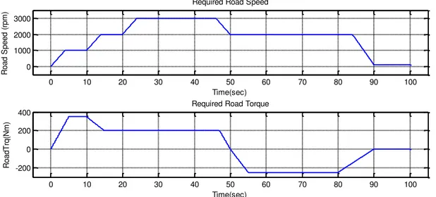
Figure 3. Speed and torque values for the simulation.

The required road speed is a plot of a combination of step by step increases and decreases with a partly constant positive speed, while the required road torque consists of the plots of both the positive and negative sides. The drive cycle is designed in such a way as to observe the power flow during both motoring and regeneration.

RESULTS AND DISCUSSION

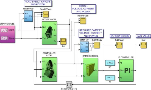
Figure 4 illustrates the EV drive simulation model produced from mathematical Eqs. (1)–[12] which are represented by each subsystem block. From the model, five simulation points were selected and added to the output scopes in order to determine and illustrate the energy flow, performance and efficiency of two important elements of the EV drive train: (i) the motor, and (ii) the battery. The simulation points are labelled in Figure 4 (in blue) as below:

1. Road speed, torque and power 2. Motor voltage, current and power

3. Required battery voltage, current and power 4. Battery error

5. Gain value

1317

Figure 4. EV drive simulation model.

0 10 20 30 40 50 60 70 80 90 100

-1 0 1 2x 10

5

Time(sec)

R

o

a

d

P

o

w

e

r(

W

a

tt

s

)

Required Road Power

(+T)*(+S)= +P = 1st Quadrant = Motoring (-T)*(+S)= -P = 4th Quadrant = Regeneration

Figure 5. Required power.

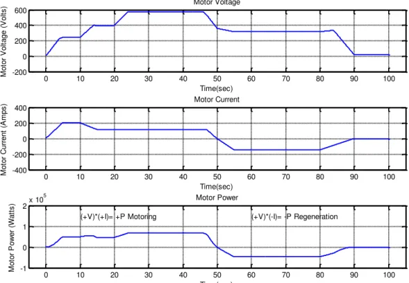
Figure 6 illustrates the voltage, current and power developed in the motor. The figure is very similar to the previous figure of speed, torque and power. The voltage curve follows the speed curve while the current follows the torque. This is obvious due to their relationship as in Eqs. (1) and (2). Finally, the power curve in the third plot,

once again confirms the motor’s operation in the motoring and regeneration modes. The

power flows from the battery to the motor during motoring operation, but returns back to the battery during regenerative braking.

1318

0 10 20 30 40 50 60 70 80 90 100

-200 0 200 400 600 Time(sec) M o to r V o lt a g e ( V o lt s

) Motor Voltage

0 10 20 30 40 50 60 70 80 90 100

-400 -200 0 200 400 Time(sec) M o to r C u rr e n t (A m p s

) Motor Current

0 10 20 30 40 50 60 70 80 90 100

-1 0 1

2x 10

5 Time(sec) M o to r P o w e r (W a tt s

) Motor Power

(+V)*(+I)= +P Motoring (+V)*(-I)= -P Regeneration

Figure 6. Motor voltage, current and power.

0 10 20 30 40 50 60 70 80 90 100

0 100 200 300 Time(sec) M o to r V o lt a g e ( V o lt s

) Battery Voltage

0 10 20 30 40 50 60 70 80 90 100

-400 -200 0 200 400 Time(sec) M o to r C u rr e n t (A m p s

) Battery Current

0 10 20 30 40 50 60 70 80 90 100

-1 0 1 2 3x 10

5 Time(sec) M o to r P o w e r (W a tt s

) Battery Power

(+V)*(+I)= +P Motoring (+V)*(-I)= -P Regeneration

Batt Energy Motoring = 745WattHour Batt Energy ReGeneration = -413WattHour

Figure 7. Battery voltage, current and power.

1319

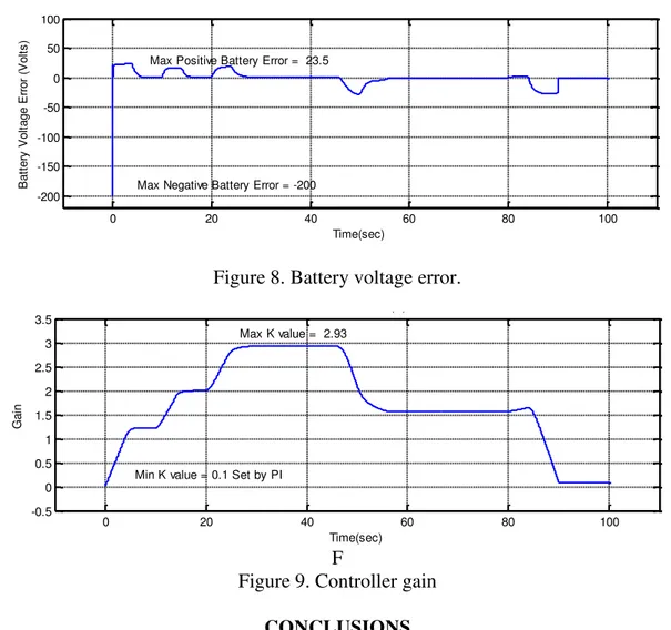
values. This error output was employed as the input to the P-I controller. From the figure, the maximum negative simulation error of -200 V which appears at 0 sec is normal and can be negligible. The controller promptly recovers the system and compensates the maximum error of 23.5 V during motor starting. The performance of the controller is acceptable because for most of the time the error is zero. However, the controller could still be improved by using various intelligent methods. The controller gain, K is presented in Figure 9. From the figure, the value of K varies proportionally to the speed demand where the rise in speed demand will increase the value of K. During modeling, the integrator in the P-I controller block is preset with 0.1 initial conditions to avoid an algebraic loop error during simulation. The P-I controller compensates the error through the selected proportional and integral constants of Kp and Ki to keep the

system healthy. The value of the constants was established from the tuning process in the Matlab-Simulink environment, providing the respective minimum and maximum K

values of 0.1 and 2.93.

0 20 40 60 80 100

-200 -150 -100 -50 0 50 100

Time(sec)

B

a

tt

e

ry

V

o

lt

a

g

e

E

rr

o

r

(V

o

lt

s

)

Max Negative Battery Error = -200 Max Positive Battery Error = 23.5

Figure 8. Battery voltage error.

0 20 40 60 80 100

-0.5 0 0.5 1 1.5 2 2.5 3 3.5

Controller Gain (K)

Time(sec)

G

a

in

Max K value = 2.93

Min K value = 0.1 Set by PI

F

Figure 9. Controller gain

CONCLUSIONS

1320

regeneration. The EV’s performance depends on the performance of the controller in removing error from the system. This work utilized a simple controller to maintain the identical input–output power of battery and the P-I controller to compensate for the voltage error. The design of the EV model presented in this paper is indeed a basic model. There are still many opportunities for augmentation in order to establish a good EV model which will form the foundation for further research and development. Modeling and simulation are very important for automotive designers in order to find the best energy control strategy and exact component size, and to minimize the use of energy, because prototyping and testing are expensive and complex operations. Good design leads to a good compromise among flexibility, model simplicity, computational load and detailed representation of the components.

ACKNOWLEDGEMENTS

The authors would like to express highest gratitude to the Faculty of Engineering, Universiti Putra Malaysia (UPM) for providing the effective facilities and efficient learning environment in conducting the research. The research is supported by the research grant of 03-01-13-1245FR from Ministry of Higher Education, Malaysia.

REFERENCES

[1] Trigg T, Telleen P, Boyd R, Cuenot F, D’Ambrosio D, Gaghen R, et al. Global EV outlook: understanding the electric vehicle landscape to 2020. International Energy Agency. 2013:1-40.

[2] Situ L. Electric vehicle development: the past, present & future. 3rd International Conference on Power Electronics Systems and Applications. 2009; 1-3.

[3] Rahmat MS, Ahmad F, Mat Yamin AK, Aparow VR, Tamaldin N. Modeling and torque tracking control of permanent magnet synchronous motor (PMSM) for hybrid electric vehicle. International Journal of Automotive and Mechanical Engineering. 2013;7:955-67.

[4] Salleh I, Md. Zain MZ, Raja Hamzah RI. Evaluation of annoyance and suitability of a back-up warning sound for electric vehicles. International Journal of Automotive and Mechanical Engineering. 2013;8:1267-77.

[5] Pereirinha PG, Trovão JP. Multiple energy sources hybridization: the future of electric vehicles?2012.

[6] Butler KL, Ehsani M, Kamath P. A Matlab-based modeling and simulation package for electric and hybrid electric vehicle design. IEEE Transactions on Vehicular Technology. 1999;48:1770-8.

[7] Husain I, Islam MS. Design, modeling and simulation of an electric vehicle system. SAE Technical Paper No. 1999-01-1149; 1999.

[8] Markel T, Brooker A, Hendricks T, Johnson V, Kelly K, Kramer B, et al. ADVISOR: a systems analysis tool for advanced vehicle modeling. Journal of Power Sources. 2002;110:255-66.

1321

[10] Kaloko BS, Soebagio MHP, Purnomo MH. Design and Development of Small Electric Vehicle using MATLAB/Simulink. International Journal of Computer Applications. 2011;24:19-23.

[11] Schaltz E. Electrical Vehicle Design and Modeling. In: Soylu S, editor. Electric Vehicles - Modelling and Simulations: InTech; 2011.

[12] Mapelli FL, Tarsitano D. Modeling of full electric and hybrid electric vehicles. INTECH Open Access Publisher; 2012.

[13] Sanita CS, Kuncheria JT. Modelling and Simulation of four Quadrant operation of Three phase Brushless DC Motor with Hysteresis Current Controller. International Journal of Advanced Research in Electrical, Electronics and Instrumentation Engineering. 2013;2:2461-70.