Volume 30, Issue 3
Diffusion Paths: Fixed Points, Periodicity and Chaos
Orlando Gomes ISCAL-IPL; UNIDE-ISCTE
Abstract
It is common to recognize that ideas, technology and information disseminate across the economy following some kind of diffusion pattern. Typically, the process of adopting a new piece of knowledge will be translated into an s-shaped trajectory for the adoption rate. This type of process of diffusion tends to be stable in the sense that convergence from any initial state towards the long-term scenario in which all the potential adopters enter in contact with the innovation is commonly guaranteed. Here, we introduce a mechanism under which stability of the diffusion process does not necessarily hold. When the perceived law of motion concerning the evolution of the number of potential adopters differs from the actual law of motion, and agents try to learn this law resorting to an adaptive learning rule, nonlinear long-term outcomes might emerge: the percentage of individuals accepting the innovation in the long-run may be a varying value that evolves according to some cyclical (periodic or a-periodic) pattern. The concept of nonlinear diffusion that is addressed is applied to a problem of information and monetary policy.
Citation: Orlando Gomes, (2010) ''Diffusion Paths: Fixed Points, Periodicity and Chaos'', Economics Bulletin, Vol. 30 no.3 pp. 2413-2424. Submitted: Aug 07 2010. Published: September 16, 2010.
1
Introduction
The establishment of economic and social relations allows ideas, knowledge, technology, infor-mation and other intangible entities to spread throughout the interested audiences. At …rst, because few have yet adopted the innovation, its rate of growth is slow, but it will evolve at an increasing pace; at some stage of this di¤usion process, the acceleration phase is typically exhausted and the rate of adoption becomes less intense as the system asymptotically con-verges to the point representing full adoption. Thus, di¤usion is characterized by an s-shaped trajectory for the variable representing the rate of adoption.
Adoption processes have been studied by the economic science under multiple scenarios. Without intending to be exhaustive, we mention some illustrative examples. A …rst important model of di¤usion is the contagion model, used by Bass (1969, 1980) to address the adoption by costumers of new consumption goods; the main idea underlying this model relates to the fact that economic agents tend to adopt an innovation whenever they perceive that others have done the same, i.e., there will be a contagion or an epidemic e¤ect. Following this pioneer work, most of the literature on di¤usion concentrates on technology adoption, both in general terms and also relating some speci…c realities. Relevant generic approaches to the di¤usion of technology include, among others, Parente (1994, 2000), Karshenas and Stoneman (1995), Geroski (2000), Chatterjee and Hu (2004) and Mukoyama (2006). An example of technology di¤usion in a speci…c sector is Barros and Martinez-Giralt (2009) who address technological di¤usion in health care.
Nevertheless, di¤usion processes are not circumscribed to technology adoption. We …nd, more generally, this type of process associated with social interaction; di¤usion of ideas and information inside social networks is a progressively more important theme of discussion by economists. Di¤usion in social networks, involving learning or a simple process of in‡uence through direct contact are addressed, e.g., in the work of Bala and Goyal (1998), Young (2003), Cowan and Jonard (2004), Jackson and Yariv (2007) and Richiardi, Gallegati, Greenwald and Stiglitz (2008). Also in macroeconomics, di¤usion assumes a relevant role; for instance, Carroll (2006) o¤ers an explanation for infrequent information updating [that is present in the sticky information macro model of Mankiw and Reis (2002, 2006, 2007)] that involves contagion: information spreads across the population as an infectious disease, i.e., under a contagion e¤ect that will imply a typical di¤usion process.
The question we ask here is whether convergence to total adoption (or, eventually in some cases, divergence back to a zero adoption level) is the only possible long-term outcome for a typical di¤usion process. Assuming a particular bounded rationality setting, we formulate an environment in which agents fail in automatically perceiving the dimension of the interested audience; as a result, they consider a perceived law of motion for the dynamics of the share of potential adopters that eventually di¤ers from the actual law of motion. Estimating the relevant parameter by resorting to an adaptive learning algorithm (involving a constant gain sequence), one may …nd a nonlinear outcome for the long-term share of agents virtually interested in adopting the innovation. The nonlinearity in potential adoption spills over actual adoption and, in the long-run, we will not be able to …nd a stable constant share of agents accepting the innovation: this value can change systematically, following either a periodic or an a-periodic pattern of evolution. There is no guarantee that the number of long-term adopters will match the initially predicted quantity of adopters; long-term observed values can be below or above the forecasted level.
If di¤usion processes lead to ’boundedly unstable’ long-term outcomes, this implies that …rms, households or public authorities will experience di¢ culties in formulating plans or poli-cies. For instance, …rms may lack the ability to predict the pro…tability of a new product or monetary authorities may …nd it harder to implement policies aimed at stabilizing prices. Af-ter characAf-terizing the process through which nonlinear di¤usion may occur, we illustrate this process by developing an example involving price setting and the role of monetary policy.
The paper is organized as follows. Section 2 selects a speci…c type of di¤usion process and applies to it the adaptive learning regime. In section 3, we study the underlying dynamics. Section 4 develops the monetary policy example and section 5 concludes.
2
The Di¤usion Process
There are several types of dynamic rules that de…ne s-shaped di¤usion processes. For instance, Young (2009) makes reference to three sources of di¤usion: by contagion, by social in‡uence or by social learning. We will consider the intermediate case - social in‡uence. In this case, each agent will intend to adopt only after a given share of agents have already adopted the innovation.
Let nt 2 [0; 1] be the share of agents that at time t have adopted the innovation and consider
the cumulative distribution function of this share, F (nt). The percentage of agents who are
willing to adopt but have not done so at time t will be entF (nt) nt, with ent2 [0; 1] the share
of potential adopters. Variable ent will correspond to the ratio of potential adopters at time t
(Nt) relatively to the entire population, which we represent by the constant level eN.
De…ning a rate of adoption 2 (0; 1), the rule governing the di¤usion process will be
nt+1 nt= [entF (nt) nt] ; n0 = 0 (1)
Independently of the considered type of distribution, F : [0; 1] ! [0; 1] and F0 > 0. Note
that F0 represents the probability density function of nt.
We assume that the number of individual agents potentially interested in adopting the new
technology or piece of information evolves in time from a given N0 value towards a steady-state
amount N Ne. This evolution process is stable and it will be presented under the form of a
simple di¤erence equation,
Nt+1 = aNt+ (1 a)N ; 0 < a < 1 (2)
Dividing both sides of equation (2) by eN, we can write the equation under the form
ent+1= aent+ (1 a)n (3)
where n := N = eN. Equation (3) is the actual law of motion (ALM) for the share of interested
individuals. Assuming a scenario of perfect foresight, agents know that (3) e¤ectively charac-terizes the evolution of the number of agents that are potentially attentive to how the adoption
rate evolves. Thus, for instance if en0 < n , then ent grows positively in time; simultaneously,
nt, i.e., the e¤ective share of adopters, will grow as well. In the long-run, the adoption share
will remain at n . Note that, in these circumstances, this is a stable outcome. Equation (3)
converge to the long-run value nt= n , i.e., in the steady-state the percentage of agents willing to absorb the ideas / knowledge / news will e¤ectively absorb them.
Now assume that the interested audience ignores the true shape of equation (3). Agents
understand that there is an initial share of potentially interested individuals, en0, but they fail
in perceiving that this number converges to n . Instead, they will expect a long-term outcome
n that may be distinct from n . The perceived law of motion (PLM) is:
Etent+1 = bent+ (1 b)n , 0 < b < 1 (4)
Parameter b represents the expected rate of convergence towards n , which agents do not
know but will try to estimate by observing the time evolution of nt. The estimation will involve
the following learning rule [in Gomes (2009), similar types of learning rules are explored],
bt+1= bt+ (bt 1 bt), 0 1 (5)
Equation (5) translates an adaptive learning process under constant gain. Basically, the expression indicates that the extent of the change in the value of b will depend on how is the
previous period change weighted. Parameter re‡ects how demanding is the learning process;
if = 0, no adjustment is required and b remains constant (this will be the perfect foresight
case, where agents possess the su¢ cient information to take as granted that the actual value of the parameter is the one already considered and no further adjustment is necessary). The
higher the value of , the larger will be the impact of previous changes in the value of b over
the current change.
According to the PLM, bt = Etnenet+1t n n ; observe that the value of b in period t 1 will be
known in t and corresponds to bt 1= enentt1nn . The learning rule can rewritten as
Et+1ent+2 n ent+1 n = Etent+1 n ent n + ent n ent 1 n Etent+1 n ent n (6)
Equation (6) corresponds to how the evolution of ent will be perceived by the economic
agents. This is the rule they will incorporate in their behavior. However, in period t + 1, the
expectation Etent+1 will correspond to the observed value of ent+1 (which is given by the ALM).
As a result, the motion of ent that agents will consider relevant to take their adoption decisions
is (6) with Etent+1=ent+1. The observed motion of ent will be given by the pair of equations
ent+1= xxtt 1an +x1 at an
zt+1 =ent
(7)
with xt:= (1 )aent+(1 a)nnet n n + enztt nn .
3
Local and Global Dynamics
We need to study the dynamic properties of (7) in order to obtain insights about the value that the share of potential adopters will, in fact, display. We begin by addressing local dynamics.
The steady-state corresponds to the point ent = z = n . System (7) can be linearized in the
vicinity of this point; we get,
ent+1 n zt+1 n = 1 1 a 1 a 1 0 : ent n zt n (8)
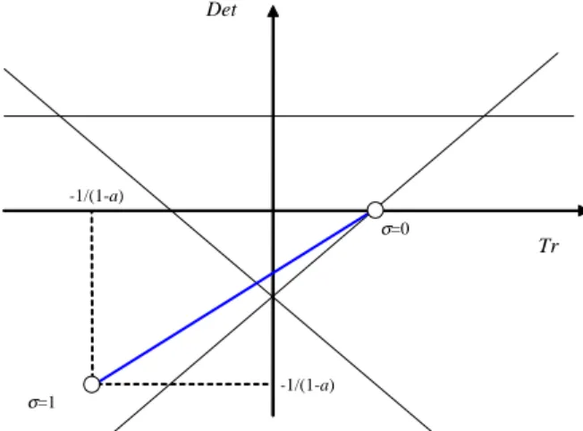
Trace and determinant of the matrix in the linearized system are, respectively, T r = 1
1 a and Det = 1 a. Stability conditions are straightforward to compute:
(i ) 1 Det = 1 +1 a > 0;
(ii ) 1 T r + Det = > 0;
(iii ) 1 + T r + Det = 2 21 a > 0
The …rst two conditions are satis…ed for any admissible value of parameters and a. The
third condition may not hold. Stability is guaranteed under the inequality < 2(1 a)3 a . At point
= 2(1 a)3 a a ‡ip bifurcation will occur. Therefore, convergence of ent to n will require a low value for the gain parameter; if a relatively large weight is attributed to previous changes when estimating future values of the parameter in the PLM, the system may be pushed into a region of absence of local stability.
Figure 1 illustrates local dynamics through the presentation of a trace-determinant diagram. The inverted triangle will correspond to the area of stability (it is the area delimited by the three bifurcation lines); the line in bold represents the dynamics of the system (the pairs trace-determinant that are admissible for di¤erent values of the gain value). One can observe that
for low values of stability is evidenced; large values of make the system fall outside the
stability area. σ=1 -1/(1-a) σ=0 -1/(1-a) Det Tr
Figure 1. Local Stability in a Trace-Determinant Diagram
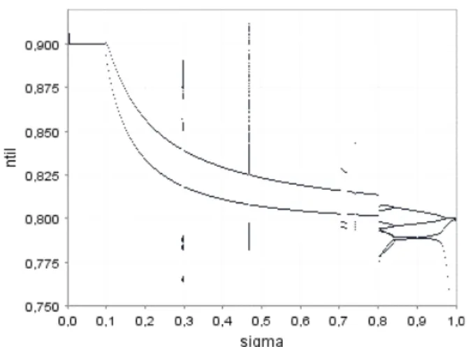
Looking at global dynamics, one observes that once stability is lost, cycles of various peri-odicities are formed for di¤erent values of . Figure 2 displays a bifurcation diagram drawn for
a = 0:9. According to the stability condition, stability holds for any value of below 0:0952;
above this value, we observe the presence of cycles of various periodicities and even the existence
of small regions of chaotic motion. Thus, ent may not remain at the constant steady-state level
(in the …gure this is n = 0:9) and, due to the learning process, the share of potential adopters may register an evolution characterized by the persistence of regular or irregular cycles. In panel B of …gure 2, a segment of the bifurcation diagram where chaotic motion is identi…ed is displayed in detail.
Figure 2. Panel A. Bifurcation diagram (0 < < 1).
Figure 2. Panel B. Bifurcation diagram (0:2865 < < 0:303).
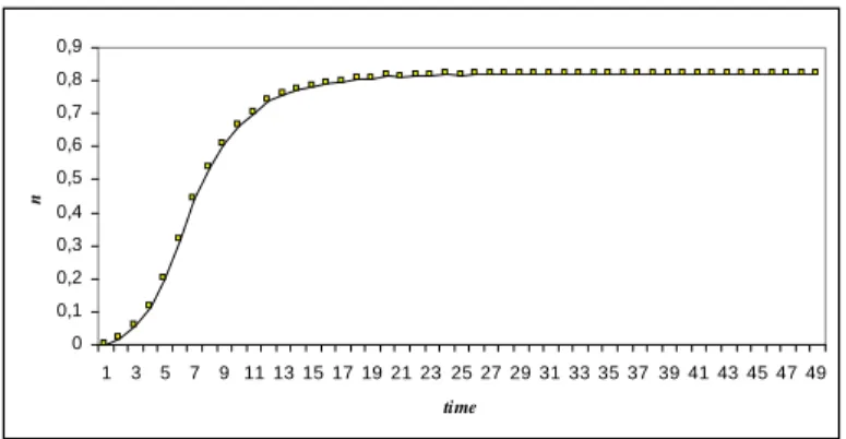
If the target that the di¤usion process intends to ful…ll is a moving target, then there will not be convergence towards a given constant number of adopters. Figure 3 displays the outcome for
nt when the gain parameter takes the value = 0:4 (and, thus, a period-2 cycle is evidenced);
recall that the motion of nt is given by equation (1). To build the trajectory for nt, we have
considered a normal distribution with mean equal to 0:1 and variance equal to 0:01. Note that
because ent is subject to endogenous ‡uctuations, a same type of nonlinear evolution is passed
on to the e¤ective adoption share. Two panels are displayed; panel A respects to the …rst 50
observations of nt; through this panel, we can con…rm the s-shaped pattern of the adoption
process. Panel B displays 50 observations after excluding the transient phase; we observe that
the long-term evolution is characterized by a period-2 cycle with ntassuming, alternatively, the
0 0,1 0,2 0,3 0,4 0,5 0,6 0,7 0,8 0,9 1 3 5 7 9 11 13 15 17 19 21 23 25 27 29 31 33 35 37 39 41 43 45 47 49 time n
Figure 3. Panel A. Di¤usion process (…rst 50 observations).
0,817 0,8175 0,818 0,8185 0,819 0,8195 0,82 0,8205 0,821 0,8215 0,822 1 4 7 10 13 16 19 22 25 28 31 34 37 40 43 46 49 time n
Figure 3. Panel B. Di¤usion process (long-run behavior).
4
The Monetary Policy Example
To illustrate the nonlinear di¤usion result, we apply it to the role of monetary policy in a setting where information about price evolution disseminates gradually across the economy.
Monetary policy will be characterized by the selection of some rate of money growth. The
initial policy will be such that money supply grows at the constant rate m0; at a given time
moment, the central bank changes its policy by increasing (or decreasing) its rate of growth
of money supply to m1. Firms will set prices at time t to the subsequent time period, given
their expectations about price evolution.
Two types of expectations are formed: agents who have not yet perceived the change in policy will expect prices to move as they did until the previous time moment, i.e., they form
an expectation EtIpt+1 = pt+ m0, with pt the price level at t, measured in logs. The …rms
that are able to understand how the policy has shifted will form rational expectations, i.e.,
EII
t pt+1= pt, where pt represents the target price …rms intend to set under a monopolistically
competitive environment [see Mankiw and Reis (2002) for details on the formation of this target
price]. The target price is de…ned by pt = pt+ yt, where ytis the output gap (the di¤erence, in
logs, between e¤ective and potential output) and > 0 is a parameter representing the degree
of real rigidities or the extent in which the di¤erent varieties of the assumed good are more or
less close from being perfect substitutes (perfect substitutability is represented by = 0). The
value of pt is chosen optimally by pro…t maximizing …rms and it indicates how …rms react to
di¤erent stages of the business cycles: phases of expansion push desired prices upward, while phases of recession imply a downward movement of desired prices.
At time t, a share nt of …rms will be acquainted with the policy change while the remainder
share 1 nt will continue to set prices as if the policy had not changed (and therefore
re-optimization is not needed). The aggregate price level at time t + 1 will be
pt+1 = (1 nt)EtIpt+1+ ntEtIIpt+1 (9)
Given the expectations formation rules, and de…ning the in‡ation rate as t := pt pt 1,
it is straightforward to transform the price level in expression (9) into a Phillips curve (into a relation between the output gap and the in‡ation rate):
t+1=
nt
1 nt
yt+1+ m0 (10)
Equation (10) can be interpreted as follows: the larger is the share of agents that, at time t, has already acknowledged the change in policy, the steeper will be the relation, at time t + 1, between the output gap and the in‡ation rate.
Next, assume a simple money demand equation mt = yt+ pt (demand for money equals
nominal output). If the policy change has already occurred, we can apply …rst di¤erences to this equation to notice that the change in the output gap will correspond to the di¤erence between
monetary growth and price change, i.e., yt+1 yt= m1 t+1. Combining this relation with
equation (10), we compute a rule of motion for the in‡ation rate:
t+1=
nt 1nt m1 (nt nt 1) m0+ (1 nt 1)nt t
nt 1[1 (1 )nt]
(11)
Equation (11) reveals the relevant role of information acquisition when assessing the dy-namics of the in‡ation rate. The share of …rms that absorb information about monetary policy changes is crucial in determining the path of in‡ation.
If one assumes that share nt evolves as characterized in section 3, the eventual nonlinear
motion of the adoption rate spills over the long-term in‡ation trajectory. In this case, the lack of price stability will be the outcome of an unstable information di¤usion process that does not allow for the number of …rms that accept the information about the new policy as reliable to be a constant value.
Let us …rst look at the steady-state. Taking := t+1 = t and applying this condition
to expression (11), we get = m1. Thus, the initial level of in‡ation will correspond to
the rate of money growth before the policy change: 0 = m0; in the long-run, the
in‡a-tion rate will coincide with the new money supply growth rate (if the steady-state is a stable point). The convergence from one to the other …xed point will occur gradually, as the di¤u-sion process implies a progressive adoption of the new information by the interested audience. The Phillips curve equation (10) allows us to determine the steady-state for the output gap: y = 1 1 n
n ( m1 m0); assuming m1 > m0, the steady-state output gap remains positive
as long as n < 1. If all the population accesses the new information, then the output gap falls to zero.
The long-run in‡ation and output gap trajectories are dependent on the speci…cation of the information di¤usion process. If we consider the learning environment, the long-term outcome for the rate of in‡ation and for the output gap will correspond to a …xed-point, periodic cycles or chaos if each of these is also the outcome of the di¤usion process. De…ciencies in e¢ ciently learning the number of agents that are e¤ectively interested in some piece of information, may
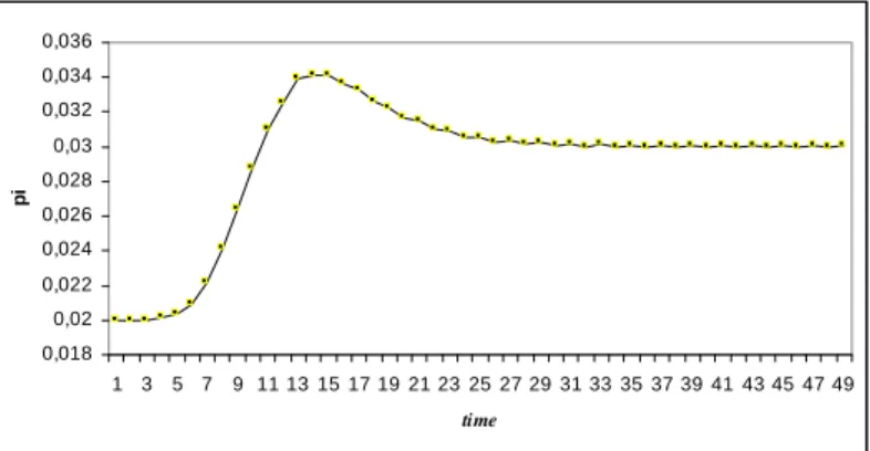
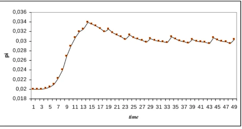
lead to nonlinear outcomes for both in‡ation and real economic activity measures. Figure 4 illustrates the result for the in‡ation rate. The example is the same used to draw …gure 3, i.e.,
we consider = 0:4 and, therefore, the long-term outcome is characterized by a period-2 cycle
(in this case, the in‡ation rate switches between 0:02992 and 0:03007); in this example, it is
also considered that m0 = 0:02 and m1 = 0:03. Panel A shows the transient phase, where
the information di¤usion process implies an in‡ation ’overshooting’; the long-run result (shown in panel B) reveals that, in fact, a period-2 cycle is followed. It is relevant to observe that the in‡ation rate ‡uctuates around the long-term growth rate of money supply, which is 0:03.
0,018 0,02 0,022 0,024 0,026 0,028 0,03 0,032 0,034 0,036 1 3 5 7 9 11 13 15 17 19 21 23 25 27 29 31 33 35 37 39 41 43 45 47 49 time pi
Figure 4. Panel A. The e¤ect of a monetary policy change over the in‡ation rate (…rst 50
observations; = 0:4). 0,02985 0,0299 0,02995 0,03 0,03005 0,0301 1 4 7 10 13 16 19 22 25 28 31 34 37 40 43 46 49 time pi
Figure 4. Panel B. The e¤ect of a monetary policy change over the in‡ation rate (long-run
impact; = 0:4).
Again, we must stress that the cycles of periodicity 2 are the direct result of assuming a learning process that allows information to spread across the population under such pattern; other gain values can imply …xed-point stability, cycles of periodicity larger than two, or fully irregular cycles. As an illustration recover the panel B of section 2. There, chaotic motion is
observed for a small range of values of . Consider a value of this constant for which chaos
e¤ectively holds; e.g., let = 0:298. Figure 5 shows the pattern of evolution for the in‡ation
rate in this speci…c case - panel A characterizes the initial phase of the adjustment process
(with 0 = m0 = 0:02); panel B displays the long-run endogenous irregular behavior of the
0,018 0,02 0,022 0,024 0,026 0,028 0,03 0,032 0,034 0,036 1 3 5 7 9 11 13 15 17 19 21 23 25 27 29 31 33 35 37 39 41 43 45 47 49 time pi
Figure 5. Panel A. The e¤ect of a monetary policy change over the in‡ation rate (…rst 50
observations; = 0:298). 0,0285 0,029 0,0295 0,03 0,0305 0,031 0,0315 1 3 5 7 9 11 13 15 17 19 21 23 25 27 29 31 33 35 37 39 41 43 45 47 49 time pi
Figure 5. Panel B. The e¤ect of a monetary policy change over the in‡ation rate (long-run
impact; = 0:298).
5
Conclusion
Di¤usion processes usually explain how some innovation becomes pervasively accepted by the economic system. Social in‡uence may justify an s-shaped adoption curve that culminates in a stable outcome where all the potential adopters end up, sooner or later, gaining access to the new idea, news or technological knowledge. This steady-state …xed-point result can be disturbed when agents fail in perceiving how the potential audience evolves over time; this value can be learned on the aggregate, but misspeci…cation problems may lead to the adoption of an incorrect learning rule. The result is that the steady-state outcome is no longer guaranteed. In the long-run, the share of agents that are potential adopters will systematically change, with some regularity or following completely irregular paths. The systematic change in the share of potential adopters automatically suggests that the long-term share of e¤ective adopters will also su¤er the same type of ‡uctuations. Once we adapt these notions about di¤usion to a speci…c economic setting (e.g., the dissemination of information on a monetary policy change over the universe of price-setting …rms), we o¤er a possible rationale for observed ‡uctuations in the economic system.
References
[1] Bala, V. and S. Goyal (1998) “Learning from Neighbours.” Review of Economic Studies 65, 595-621.
[2] Barros, P. P. and X. Martinez-Giralt (2009) "Technological Adoption in Health Care." Universidade Nova de Lisboa and Universitat Autonoma de Barcelona working paper. [3] Bass, F. (1969) "A New Product Growth Model for Consumer Durables." Management
Science 15, 215-227.
[4] Bass, F. (1980) "The Relationship between Di¤usion Rates, Experience Curves and De-mand Elasticities for Consumer Durables and Technological Innovations." , Journal of Business 53, 551-567.
[5] Carroll, C. D. (2006) "The Epidemiology of Macroeconomic Expectations." in L. Blaume and S. Durlauf (eds.), The Economy as an Evolving Complex System III, Oxford: Oxford University Press.
[6] Chatterjee, K. and S. Hu (2004) "Technology Di¤usion by Learning from Neighbors." Advances in Applied Probability 36, 355-376.
[7] Cowan, R. and N. Jonard (2004) “Network Structure and the Di¤usion of Knowledge.” Journal of Economic Dynamics and Control 28, 1557-1575.
[8] Geroski, P. A. (2000) "Models of Technology Di¤usion." Research Policy 29, 603–625. [9] Gomes, O. (2009) "Adaptive Learning and Complex Dynamics." Chaos, Solitons and
Frac-tals 42, 1206-1213.
[10] Jackson, M. O. and L. Yariv (2007) “Di¤usion of Behavior and Equilibrium Properties in Network Games.” American Economic Review Papers and Proceedings 97, 92-98.
[11] Karshenas, M. and P. Stoneman (1995) "Technological Di¤usion." in: Stoneman, P. (Ed.), Handbook of the Economics of Innovation and Technological Change. Oxford: Blackwell, 265–297.
[12] Mankiw, N. G. and R. Reis (2002) "Sticky Information versus Sticky Prices: a Proposal to Replace the New Keynesian Phillips Curve." Quarterly Journal of Economics 117, 1295-1328.
[13] Mankiw, N. G. and R. Reis (2006) "Pervasive Stickiness." American Economic Review 96, 164-169.
[14] Mankiw, N. G. and R. Reis (2007) "Sticky Information in General Equilibrium." Journal of the European Economic Association 5, 603-613.
[15] Mukoyama, T. (2006) "Rosenberg’s ’Learning by Using’and Technology Di¤usion." Jour-nal of Economic Behavior and Organization 61, 123-144.
[16] Parente, S. L. (1994) "Technology Adoption, Learning-by-doing, and Economic Growth." Journal of Economic Theory 63, 346-369.
[17] Parente, S. L. (2000) "Learning-by-using and the Switch to Better Machines." Review of Economic Dynamics 3, 675-703.
[18] Gallegati, M.; B. Greenwald; M. G. Richiardi; and J. E. Stiglitz (2008) "The Asymmetric E¤ect of Di¤usion Processes: Risk Sharing and Contagion." Global Economy Journal 8, Issue 3, Article 2.
[19] Young, H. P. (2003) “The Di¤usion of Innovations in Social Networks.” in The Economy as a Complex Evolving System, vol. III, ed. L. E. Blume and S. N. Durlauf. Oxford: Oxford University Press.
[20] Young, H. P. (2009) "Innovation Di¤usion in Heterogeneous Populations: Contagion, Social In‡uence, and Social Learning." American Economic Review 99, 1899-1924.