An Effective Implementation of the
Lin-Kernighan Traveling Salesman Heuristic
Keld Helsgaun E-mail: [email protected] Department of Computer Science
Roskilde University DK-4000 Roskilde, Denmark
Abstract
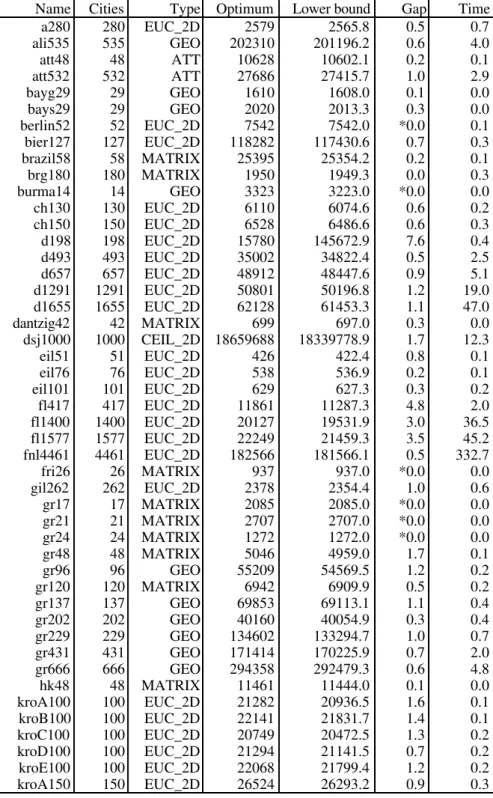
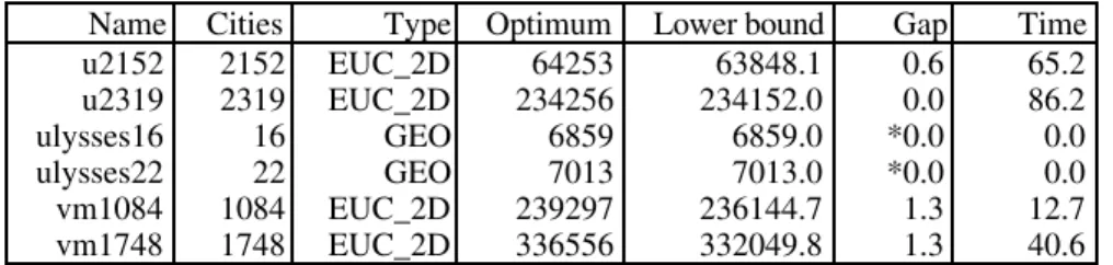
This report describes an implementation of the Lin-Kernighan heuris-tic, one of the most successful methods for generating optimal or near-optimal solutions for the symmetric traveling salesman problem. Com-putational tests show that the implementation is highly effective. It has found optimal solutions for all solved problem instances we have been able to obtain, including a 7397-city problem (the largest nontrivial problem instance solved to optimality today). Furthermore, the algo-rithm has improved the best known solutions for a series of large-scale problems with unknown optima, among these an 85900-city problem.
1. Introduction
The Lin-Kernighan heuristic [1] is generally considered to be one of the most effective methods for generating optimal or near-optimal solutions for the symmetric traveling salesman problem. However, the design and implemen-tation of an algorithm based on this heuristic is not trivial. There are many design and implementation decisions to be made, and most decisions have a great influence on performance.
This report describes the implementation of a new modified version of the Lin-Kernighan algorithm. Computational experiments have shown that the implementation is highly effective.
Run times of both algorithms increase approximately as n2.2. However, the
new algorithm is much more effective. The new algorithm makes it possible to find optimal solutions to large-scale problems, in reasonable running times. For a typical 100-city problem the optimal solution is found in less than a sec-ond, and for a typical 1000-city problem optimum is found in less than a min-ute (on a 300 MHz G3 Power Macintosh).
2. The traveling salesman problem 2.1 Formulation
A salesman is required to visit each of n given cities once and only once, starting from any city and returning to the original place of departure. What tour should he choose in order to minimize his total travel distance?
The distances between any pair of cities are assumed to be known by the salesman. Distance can be replaced by another notion, such as time or money. In the following the term ’cost’ is used to represent any such notion.
This problem, the traveling salesman problem (TSP), is one of the most widely studied problems in combinatorial optimization [2]. The problem is easy to state, but hard to solve. Mathematically, the problem may be stated as follows:
Given a ‘cost matrix’ C = (cij), where cij represents the cost of
going from city i to city j, (i, j = 1, ..., n), find a permutation (i1, i2, i3, ..., in) of the integers from 1 through n that minimizes
the quantity
ci1i2 + ci2i3 + ... + cini1
Properties of the cost matrix C are used to classify problems.
• If cij = cji for all i and j, the problem is said to be symmetric; otherwise, it
is asymmetric.
• If the triangle inequality holds (cik≤ cij + cjk for all i, j and k), the problem
is said to be metric.
• If cij are Euclidean distances between points in the plane, the problem is
said to be Euclidean. A Euclidean problem is, of course, both symmetric and metric.
2.2 Motivation
For example, consider the following process planning problem. A number of jobs have to be processed on a single machine. The machine can only process one job at a time. Before a job can be processed the machine must be prepared (cleaned, adjusted, or whatever). Given the processing time of each job and the switch-over time between each pair of jobs, the task is to find an execu-tion sequence of the jobs making the total processing time as short as possi-ble.
It is easy to see that this problem is an instance of TSP. Here cij represents the time to complete job j after job i (switch-over time plus time to perform job j). A pseudo job with processing time 0 marks the beginning and ending state for the machine.
Many real-world problems can be formulated as instances of the TSP. Its ver-satility is illustrated in the following examples of application areas:
• Computer wiring • Vehicle routing • Crystallography • Robot control
• Drilling of printed circuit boards • Chronological sequencing.
TSP is a typical problem of its genre: combinatorial optimization. This means that theoretical and practical insight achieved in the study of TSP can often be useful in the solution of other problems in this area. In fact, much progress in combinatorial optimization can be traced back to research on TSP. The now well-known computing method, branch and bound, was first used in the context of TSP [3, 4]. It is also worth mentioning that research on TSP was an important driving force in the development of the computational complex-ity theory in the beginning of the 1970s [5].
However, the interest in TSP not only stems from its practical and theoretical importance. The intellectual challenge of solving the problem also plays a role. Despite its simple formulation, TSP is hard to solve. The difficulty be-comes apparent when one considers the number of possible tours - an astro-nomical figure even for a relatively small number of cities. For a symmetric problem with n cities there are (n-1)!/2 possible tours. If n is 20, there are more than 1018 tours. The 7397-city problem, which is successfully solved
by the algorithm described in this report, contains more than 1025,000 possible
2.3 Solution algorithms
It has been proven that TSP is a member of the set of NP-complete problems. This is a class of difficult problems whose time complexity is probably expo-nential. The members of the class are related so that if a polynomial time were found for one problem, polynomial time algorithms would exist for all of them. However, it is commonly believed that no such polynomial algorithm exists. Therefore, any attempt to construct a general algorithm for finding op-timal solutions for the TSP in polynomial time must (probably) fail.
That is, for any such algorithm it is possible to construct problem instances for which the execution time grows at least exponentially with the size of the input. Note, however, that time complexity here refers to any algorithm’s be-havior in worst cases. It can not be excluded that there exist algorithms whose average running time is polynomial. The existence of such algorithms is still an open question.
Algorithms for solving the TSP may be divided into two classes: • Exact algorithms;
• Approximate (or heuristic) algorithms. 2.3.1 Exact algorithms
The exact algorithms are guaranteed to find the optimal solution in a bounded number of steps. Today one can find exact solutions to symmetric problems with a few hundred cities, although there have been reports on the solution of problems with thousands of cities.
The most effective exact algorithms are cutting-plane or facet-finding algo-rithms [6, 7, 8]. These algoalgo-rithms are quite complex, with codes on the order of 10,000 lines. In addition, the algorithms are very demanding of computer power. For example, the exact solution of a symmetric problem with 2392 cities was determined over a period of more than 27 hours on a powerful su-per computer [7]. It took roughly 3-4 years of CPU time on a large network of computers to determine the exact solution of the previously mentioned 7397-city problem [8].
2.3.2 Approximate algorithms
In contrast, the approximate algorithms obtain good solutions but do not guar-antee that optimal solutions will be found. These algorithms are usually very simple and have (relative) short running times. Some of the algorithms give solutions that in average differs only by a few percent from the optimal so-lution. Therefore, if a small deviation from optimum can be accepted, it may be appropriate to use an approximate algorithm.
The class of approximate algorithms may be subdivided into the following three classes:
• Tour construction algorithms • Tour improvement algorithms • Composite algorithms.
The tour construction algorithms gradually build a tour by adding a new city at each step. The tour improvement algorithms improve upon a tour by per-forming various exchanges. The composite algorithms combine these two features.
A simple example of a tour construction algorithm is the so-called nearest-neighbor algorithm [11]: Start in an arbitrary city. As long as there are cities, that have not yet been visited, visit the nearest city that still has not appeared in the tour. Finally, return to the first city.
This approach is simple, but often too greedy. The first distances in the con-struction process are reasonable short, whereas the distances at the end of the process usually will be rather long. A lot of other construction algorithms have been developed to remedy this problem (see for example [2], [12] and [13]).
The tour improvement algorithms, however, have achieved the greatest suc-cess. A simple example of this type of algorithm is the so-called 2-opt algo-rithm: Start with a given tour. Replace 2 links of the tour with 2 other links in such a way that the new tour length is shorter. Continue in this way until no more improvements are possible.
t
1t
2t
3t
4t
2t
1t
4t
3Figure 2.1A 2-opt move
A generalization of this simple principle forms the basis for one the most ef-fective approximate algorithms for solving the symmetric TSP, the Lin-Ker-nighan algorithm [1]. The original algorithm, as implemented by Lin and Kernighan in 1971, had an average running time of order n2.2 and was able to
3. The Lin-Kernighan algorithm 3.1 The basic algorithm
The 2-opt algorithm is a special case of the -opt algorithm [15], where in each step λ links of the current tour are replaced by λ links in such a way that a shorter tour is achieved. In other words, in each step a shorter tour is ob-tained by deleting λ links and putting the resulting paths together in a new way, possibly reversing one ore more of them.
The λ-opt algorithm is based on the concept -optimality:
A tour is said to be -optimal (or simply -opt) if it is impossible to obtain a shorter tour by replacing any λ of its links by any other set of λ links.
From this definition it is obvious that any λ-optimal tour is also λ’-optimal for 1 ≤λ’ ≤λ. It is also easy to see that a tour containing n cities is optimal if and only if it is n-optimal.
In general, the larger the value of λ, the more likely it is that the final tour is optimal. For fairly large λ it appears, at least intuitively, that a λ-optimal tour should be optimal.
Unfortunately, the number of operations to test all λ-exchanges increases rapidly as the number of cities increases. In a naive implementation the testing of a λ-exchange has a time complexity of O(nλ). Furthermore, there is no nontrivial upper bound of the number of λ–exchanges. As a result, the values
λ = 2 and λ = 3 are the most commonly used. In one study the values λ = 4 and λ = 5 were used [16].
However, it is a drawback that λmust be specified in advance. It is difficult to know what λ to use to achieve the best compromise between running time and quality of solution.
Lin and Kernighan removed this drawback by introducing a powerful variable -opt algorithm. The algorithm changes the value of λ during its execution, deciding at each iteration what the value of λ should be. At each iteration step the algorithm examines, for ascending values of λ, whether an interchange of
At each step the algorithm considers a growing set of potential exchanges (starting with r = 2). These exchanges are chosen in such a way that a feasible tour may be formed at any stage of the process. If the exploration succeeds in finding a new shorter tour, then the actual tour is replaced with the new tour. The Lin-Kernighan algorithm belongs to the class of so-called local optimiza-tion algorithms [17, 18]. The algorithm is specified in terms of exchanges (or moves) that can convert one tour into another. Given a feasible tour, the algo-rithm repeatedly performs exchanges that reduce the length of the current tour, until a tour is reached for which no exchange yields an improvement. This process may be repeated many times from initial tours generated in some randomized way. The algorithm is described below in more detail.
Let T be the current tour. At each iteration step the algorithm attempts to find two sets of links, X = {x1, ..., xr} and Y = {y1, ..., yr}, such that, if the
links of X are deleted from T and replaced by the links of Y, the result is a better tour. This interchange of links is called a r-opt move. Figure 3.1 illus-trates a 3-opt move.
y1 y3
y2
x1
x3 x2
y1 y3
y2
x2 x3
x1 Figure 3.1 A 3-opt move
The two sets X and Y are constructed element by element. Initially X and Y are empty. In step i a pair of links, xi and yi, are added to X and Y,
respec-tively.
In order to achieve a sufficient efficient algorithm, only links that fulfill the following criteria may enter X and Y.
(1) The sequential exchange criterion
xi and yi must share an endpoint, and so must yi and xi+1. If t1 denotes one of
the two endpoints of x1, we have in general: xi = (t2i-1,t2i), yi = (t2i,t2i+1) and
yi t2i+2
t2i-1 t2i+1
t2i xi yi+1 xi+1
Figure 3.2. Restricting the choice of xi, yi, xi+1, and yi+1.
As seen, the sequence (x1, y1, x2, y2, x3, ..., xr, yr) constitutes a chain of
ad-joining links.
A necessary (but not sufficient) condition that the exchange of links X with links Y results in a tour is that the chain is closed, i.e., yr = (t2r,t1). Such an
exchange is called sequential.
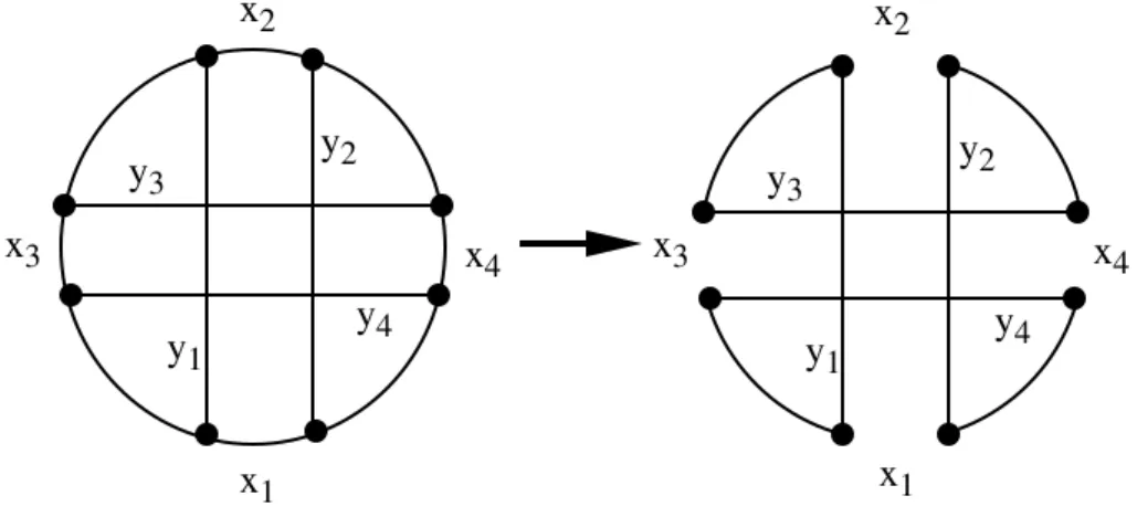
Generally, an improvement of a tour may be achieved as a sequential ex-change by a suitable numbering of the affected links. However, this is not always the case. Figure 3.3 shows an example where a sequential exchange is not possible.
Figure 3.3 Nonsequential exchange (r = 4).
y1 y4
y2 y3
y1 y4
y2 y3
x3
x2
x4
x1 x1
x2
(2) The feasibility criterion
It is required that xi = (t2i-1,t2i) is chosen so that, if t2iis joined to t1, the
re-sulting configuration is a tour. This feasibility criterion is used for i ≥ 3 and guarantees that it is possible to close up to a tour. This criterion was included in the algorithm both to reduce running time and to simplify the coding. (3) The positive gain criterion
It is required that yi is always chosen so that the gain, Gi, from the proposed
set of exchanges is positive. Suppose gi = c(xi) - c(yi) is the gain from
ex-changing xi with yi. Then Gi is the sum g1 + g2 + ... + gi.
This stop criterion plays a great role in the efficiency of the algorithm. The demand that every partial sum, Gi, must be positive seems immediately to be
too restrictive. That this, however, is not the case, follows from the following simple fact: If a sequence of numbers has a positive sum, there is a cyclic permutation of these numbers such that every partial sum is positive. The proof is simple and can be found in [1].
(4) The disjunctivity criterion
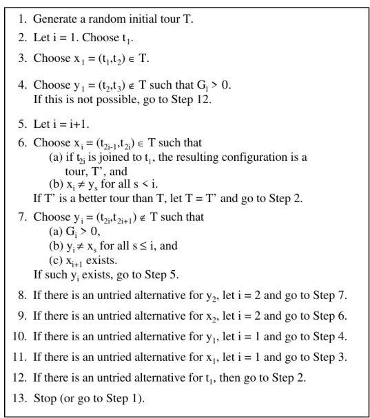
Below is given an outline of the basic algorithm (a simplified version of the original algorithm).
1. Generate a random initial tour T. 2. Let i = 1. Choose t1.
3. Choose x1 = (t1,t2) ∈ T.
4. Choose y1 = (t2,t3) ∉ T such that G1 > 0.
If this is not possible, go to Step 12. 5. Let i = i+1.
6. Choose xi = (t2i-1,t2i) ∈ T such that
(a) if t2i is joined to t1, the resulting configuration is a
tour, T’, and (b) xi≠ ys for all s < i.
If T’ is a better tour than T, let T = T’ and go to Step 2. 7. Choose yi = (t2i,t2i+1) ∉ T such that
(a) Gi > 0,
(b) yi ≠ xs for all s ≤ i, and
(c) xi+1 exists.
If such yi exists, go to Step 5.
8. If there is an untried alternative for y2, let i = 2 and go to Step 7. 9. If there is an untried alternative for x2, let i = 2 and go to Step 6. 10. If there is an untried alternative for y1, let i = 1 and go to Step 4. 11. If there is an untried alternative for x1, let i = 1 and go to Step 3. 12. If there is an untried alternative for t1, then go to Step 2.
13. Stop (or go to Step 1).
Figure 3.4. The basic Lin-Kernighan algorithm
Comments on the algorithm:
Step 1. A random tour is chosen as the starting point for the explorations. Step 3. Choose a link x1 = (t1,t2) on the tour. When t1 has been chosen, there
alter-Step 6. There are two choices of xi. However, for given yi-1 (i ≥ 2) only one
of these makes it possible to ‘close’ the tour (by the addition of yi). The other
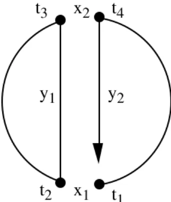
choice results in two disconnected subtours. In only one case, however, such an unfeasible choice is allowed, namely for i = 2. Figure 3.5 shows this situation.
t1 t2 x1 y1
t3 x2 t4
y2
Figure 3.5 No close up at x2.
If y2 is chosen so that t5 lies between t2 and t3, then the tour can be closed in
the next step. But then t6 may be on either side of t5 (see Figure 3.6); the
original algorithm investigated both alternatives.
t1 t2 x1
t3 t4
t5 x3
y1 y2 x2
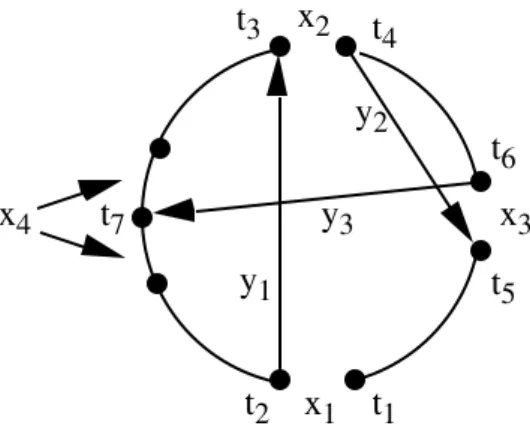
On the other hand, if y2 is chosen so that t5 lies between t4 and t1, there is only
one choice for t6 (it must lie between t4 and t5), and t7 must lie between t2 and t3. But then t8 can be on either side of t7 (see Figure 3.7); the original algo-rithm investigated the alternative for which c(t7,t8) is maximum.
t1 t2
t3 t4
t5 t6 t7
x4
x1
x3 x2
y1
y2
y3
Figure 3.7 Unique choice for x3. Limited choice of y3. Two choices for x4.
Condition (b) in Step 6 and Step 7 ensures that the sets X and Y are disjoint: yi must not be a previously broken link, and xi must not be a link previously
added.
Steps 8-12. These steps cause backtracking. Note that backtracking is al-lowed only if no improvement has been found, and only at levels 1 and 2. Step 13. The algorithm terminates with a solution tour when all values of t1
have been examined without improvement. If required, a new random initial tour may be considered at Step 1.
The algorithm described above differs from the original one by its reaction on tour improvements. In the algorithm given above, a tour T is replaced by a shorter tour T’ as soon as an improvement is found (in Step 6). In contrast, the original algorithm continues its steps by adding potential exchanges in or-der to find an even shorter tour. When no more exchanges are possible, or when Gi ≤ G*, where G* is the best improvement of T recorded so far, the
3.2 Lin and Kernighan’s refinements
A bottleneck of the algorithm is the search for links to enter the sets X and Y. In order to increase efficiency, special care therefore should be taken to limit this search. Only exchanges that have a reasonable chance of leading to a re-duction of tour length should be considered.
The basic algorithm as presented in the preceding section limits its search by using the following four rules:
(1) Only sequential exchanges are allowed. (2) The provisional gain must be positive.
(3) The tour can be ‘closed’ (with one exception, i = 2).
(4) A previously broken link must not be added, and a previously added link must not be broken.
To limit the search even more Lin and Kernighan refined the algorithm by in-troducing the following rules:
(5) The search for a link to enter the tour, yi = (t2i,t2i+1), is limited to
the five nearest neighbors to t2i.
(6) For i ≥ 4, no link, xi, on the tour must be broken if it is a common link of a small number (2-5) of solution tours.
(7) The search for improvements is stopped if the current tour is the same as a previous solution tour.
Rules 5 and 6 are heuristic rules. They are based on expectations of which links are likely to belong to an optimal tour. They save running time, but sometimes at the expense of not achieving the best possible solutions.
Rule 7 also saves running time, but has no influence on the quality of solu-tions being found. If a tour is the same as a previous solution tour, there is no point in attempting to improve it further. The time needed to check that no more improvements are possible (the checkout time) may therefore be saved. According to Lin and Kernighan the time saved in this way it typically 30 to 50 percent of running time.
chosen. In cases where several alternatives must be tried, the alternatives are tried in descending priority order (using backtracking). To be more specific, the following rules are used:
(8) When link yi (i ≥ 2) is to be chosen, each possible choice is given the priority c(xi+1) - c(yi).
(9) If there are two alternatives for x4, the one where c(x4) is highest
is chosen.
Rule 8 is a heuristic rule for ranking the links to be added to Y. The priority for yi is the length of the next (unique) link to be broken, xi+1, if yi is included
in the tour, minus the length of yi. In this way, the algorithm is provided with
some look-ahead. By maximizing the quantity c(xi+1) - c(yi), the algorithm
aims at breaking a long link and including a short link.
Rule 9 deals with the special situation in Figure 3.7 where there are two choices for x4. The rule gives preference to the longest link in this case. In
three other cases, namely for x1, x2, and sometimes x3 (see Figure 3.6) there
are two alternatives available. In these situations the algorithm examines both choices using backtracking (unless an improved tour was found). In their pa-per Lin and Kernighan do not specify the sequence in which the alternatives are examined.
4. The modified Lin-Kernighan algorithm
Lin and Kernighan’s original algorithm was reasonably effective. For prob-lems with up to 50 cities, the probability of obtaining optimal solutions in a single trial was close to 100 percent. For problems with 100 cities the prob-ability dropped to between 20 and 30 percent. However, by running a few trials, each time starting with a new random tour, the optimum for these problems could be found with nearly 100 percent assurance.
The algorithm was evaluated on a spectrum of problems, among these a drill-ing problem with 318 points. Due to computer-storage limitations, the prob-lem was split into three smaller probprob-lems. A solution tour was obtained by solving the subproblems separately, and finally joining the three tours. At the time when Lin and Kernighan wrote their paper (1971), the optimum for this problem was unknown. Now that the optimum is known, it may be noted that their solution was 1.3 percent above optimum.
In the following, a modified and extended version of their algorithm is pre-sented. The new algorithm is a considerable improvement of the original algo-rithm. For example, for the mentioned 318-city problem the optimal solution is now found in a few trials (approximately 2), and in a very short time (about one second on a 300 MHz G3 Power Macintosh). In general, the quality of solutions achieved by the algorithm is very impressive. The algorithm has been able to find optimal solutions for all problem instances we have been able to obtain, including a 7397-city problem (the largest nontrivial problem instance solved to optimality today).
The increase in efficiency is primarily achieved by a revision of Lin and Ker-nighan’s heuristic rules for restricting and directing the search. Even if their heuristic rules seem natural, a critical analysis shows that they suffer from considerable defects.
4.1 Candidate sets
A central rule in the original algorithm is the heuristic rule that restricts the in-clusion of links in the tour to the five nearest neighbors to a given city (Rule 5 in Section 3.2). This rule directs the search against short tours and reduces the search effort substantially. However, there is a certain risk that the appli-cation of this rule may prevent the optimal solution from being found. If an optimal solution contains one link, which is not connected to the five nearest neighbors of its two end cities, then the algorithm will have difficulties in ob-taining the optimum.
neigh-bors to be considered ought to be at least 22. Unfortunately, this enlargement of the set of candidates results in a substantial increase in running time.
The rule builds on the assumption that the shorter a link is, the greater is the probability that it belongs to an optimal tour. This seems reasonable, but used too restrictively it may result in poor tours.
In the following, a measure of nearness is described that better reflects the chances of a given link being a member of an optimal tour. This measure, called -nearness, is based on sensitivity analysis using minimum spanning trees.
First, some well-known graph theoretical terminology is reviewed.
Let G = (N, E) be a undirected weighted graph where N = {1, 2, ..., n} is the set of nodes and E = {(i,j)| i ∈ N, j ∈N} is the set of edges. Each edge (i,j) has associated a weight c(i,j).
A path is a set of edges {(i1,i2), (i2,i3), ..., (ik-1,ik)} with ip≠ iq for all p ≠ q.
A cycle is a set of edges {(i1,i2), (i2,i3), ..., (ik,i1)} with ip≠ iq for p ≠ q.
A tour is a cycle where k = n.
For any subset S ⊆E the length of S, L(S), is given by L(S) = ∑(i,j)∈S c(i,j). An optimal tour is a tour of minimum length. Thus, the symmetric TSP can simply be formulated as: “Given a weighted graph G, determine an optimal tour of G”.
A graph G is said to be connected if it contains for any pair of nodes a path connecting them.
A tree is a connected graph without cycles. A spanning tree of a graph G with n nodes is a tree with n-1 edges from G. A minimum spanning tree is a span-ning tree of minimum length.
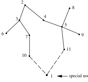
Now the important concept of a 1-tree may be defined.
The choice of node 1 as a special node is arbitrary. Note that a 1-tree is not a tree since it contains a cycle (containing node 1; see Figure 4.1).
Figure 4.1 A 1-tree.
A minimum 1-tree is a 1-tree of minimum length.
The degree of a node is the number of edges incident to the node. It is easy to see [20, 21] that
(1) an optimal tour is a minimum 1-tree where every node has degree 2; (2) if a minimum 1-tree is a tour, then the tour is optimal.
Thus, an alternative formulation of the symmetric TSP is: “Find a minimum 1-tree all whose nodes have degree 2”.
Usually a minimum spanning tree contains many edges in common with an optimal tour. An optimal tour normally contains between 70 and 80 percent of the edges of a minimum 1-tree. Therefore, minimum 1-trees seem to be well suited as a heuristic measure of ‘nearness’. Edges that belong, or ‘nearly be-long', to a minimum 1-tree, stand a good chance of also belonging to an op-timal tour. Conversely, edges that are ‘far from’ belonging to a minimum 1-tree have a low probability of also belonging to an optimal tour. In the Lin-Kernighan algorithm these ‘far’ edges may be excluded as candidates to enter a tour. It is expected that this exclusion does not cause the optimal tour to be missed.
1 10
7 6
3 2
4
8
5
9
11
More formally, this measure of nearness is defined as follows:
Let T be a minimum 1-tree of length L(T) and let T+(i,j) denote
a minimum 1-tree required to contain the edge (i,j). Then the nearness of an edge (i,j) is defined as the quantity
α(i,j) = L(T+(i,j)) - L(T).
That is, given the length of (any) minimum 1-tree, the α−nearness of an edge is the increase of length when a minimum 1-tree is required to contain this edge.
It is easy to verify the following two simple properties of α: (1) α(i,j) ≥ 0.
(2) If (i,j) belongs to some minimum 1-tree, then α(i,j) = 0.
The α-measure can be used to systematically identify those edges that could conceivably be included in an optimal tour, and disregard the remainder. These 'promising edges', called the candidateset, may, for example, consist of the k α-nearest edges incident to each node, and/or those edges having an
α-nearness below a specified upper bound.
In general, using the α-measure for specifying the candidate set is much better than using nearest neighbors. Usually, the candidate set may be smaller, without degradation of the solution quality.
The use of α-nearness in the construction of the candidate set implies com-putations of α-values. The efficiency, both in time of space, of these compu-tations is therefore important. The method is not of much practical value, if the computations are too expensive. In the following an algorithm is pre-sented that computes all α-values. The algorithm has time complexity O(n2)
and uses space O(n).
Let G = (N, E) be a complete graph, that is, a graph where for all nodes i and j in N there is an edge (i,j) in E. The algorithm first finds a minimum 1-tree for G. This can be done by determination of a minimum spanning tree that contains the nodes {2, 3, …, n}, followed by the addition of the two shortest edges incident to node 1. The minimum spanning tree may, for example, be determined using Prim’s algorithm [22], which has a run time complexity of O(n2). The additional two edges may be determined in time O(n). Thus, the
Next, the nearness α(i,j) is determined for all edges (i,j). Let T be a minimum 1-tree. From the definition of a minimum spanning tree, it is easy to see that a minimum spanning tree T+(i,j) containing the edge (i,j) may be determined
from T using the following action rules:
(a) If (i,j) belongs to T, then T+(i,j) is equal to T.
(b) Otherwise, if (i,j) has 1 as end node (i = 1 ∨j = 1), then T+(i,j) is
obtained from T by replacing the longest of the two edges of T incident to node 1 with (i,j).
(c) Otherwise, insert (i,j) in T. This creates a cycle containing (i,j) in the spanning tree part of T. Then T+(i,j) is obtained by
removing the longest of the other edges on this cycle.
Cases a and b are simple. With a suitable representation of 1-trees they can both be treated in constant time.
Case c is more difficult to treat efficiently. The number of edges in the pro-duced cycles is O(n). Therefore, with a suitable representation it is possible to treat each edge with time complexity O(n). Since O(n2) edges must be treated
this way, the total time complexity becomes O(n3), which is unsatisfactory.
However, it is possible to obtain a total complexity of O(n2) by exploiting a
simple relation between the α-values [23, 24].
Let β(i,j) denote the length of the edge to be removed from the spanning tree when edge (i,j) is added. Thus α(i,j) = c(i,j) - β(i,j). Then the following fact may be exploited (see Figure 4.2). If (j1,j2) is an edge of the minimum
span-ning tree, iis one of the remaining nodes and j1 is on that cycle that arises by adding the edge (i,j2) to the tree, then β(i,j2) may be computed as the
Figure 4.2 (i,j2) may be computed from (i,j1).
Thus, for a given node i all the values β(i,j), j = 1, 2, ..., n, can be computed with a time complexity of O(n), if only the remaining nodes are traversed in a suitable sequence. It can be seen that such a sequence is produced as a by-product of Prim’s algorithm for constructing minimum spanning trees, namely a topological order, in which every node's descendants in the tree are placed after the node. The total complexity now becomes O(n2).
Figure 4.3 sketches in C-style notation an algorithm for computing β(i,j) for i ≠ 1, j ≠ 1, i ≠ j. The algorithm assumes that the father of each node j in the tree, dad[j], precedes the node (i.e., dad[j] = i ⇒ i < j).
for (i = 2; i < n; i++) { β[i][i] = -∞;
for (j = i+1; j <= n; j++)
β[i][j] = β[j][i] = max(β[i][dad[j]], c(j,dad[j])); }
Figure 4.3 Computation of (i,j) for i ≠1, j ≠1, i j.
Unfortunately this algorithm needs space O(n2) for storing β-values. Some
space may be saved by storing the c- and β-values in one quadratic matrix, so that, for example, the c-values are stored in the lower triangular matrix, while the β-values are stored in the upper triangular matrix. For large values of n, however, storage limitations may make this approach impractical.
1 i
j1
Half of the space may be saved if the c-values are not stored, but computed when needed (for example as Euclidean distances). The question is whether it is also possible to save the space needed for the β-values At first sight it would seem that the β-values must be stored in order to achieve O(n2) time
complexity for their computation. That this is not the case will now be dem-onstrated.
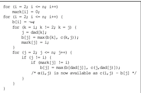
The algorithm, given in Figure 4.4, uses two one-dimensional auxiliary ar-rays, b and mark. Array b corresponds to the β-matrix but only contains β -values for a given node i, i.e., b[j] = β(i,j). Array mark is used to indicate that b[j] has been computed for node i.
The determination of b[j] is done in two phases. First, b[j] is computed for all nodes j on the path from node i to the root of the tree (node 2). These nodes are marked with i. Next, a forward pass is used to compute the re-maining b-values. The α-values are available in the inner loop.
for (i = 2; i <= n; i++) mark[i] = 0;
for (i = 2; i <= n; i++) { b[i] = -∞;
for (k = i; k != 2; k = j) { j = dad[k];
b[j] = max(b[k], c(k,j)); mark[j] = i;
}
for (j = 2; j <= n; j++) { if (j != i) {
if (mark[j] != i)
b[j] = max(b[dad[j]], c(j,dad[j)]);
/* α(i,j) is now available as c(i,j) - b[j] */ }
} }
Figure 4.4 Space efficient computation of .
It is easy to see that this algorithm has time complexity O(n2) and uses space
O(n).
c-nearest edge for a node, whereas the worst case when using the α-measure is an optimal edge being the 14th α-nearest. The average rank of the optimal edges among the candidate edges is reduced from 2.4 to 2.1.
This seems to be quite satisfactory. However, the α-measure can be improved substantially by making a simple transformation of the original cost matrix. The transformation is based on the following observations [21]:
(1) Every tour is a 1-tree. Therefore the length of a minimum 1-tree is a lower bound on the length of an optimal tour.
(2) If the length of all edges incident to a node are changed with the same amount, π, any optimal tour remains optimal. Thus, if the cost matrix C= (cij) is transformed to D = (dij), where
dij = cij + πi + πj,
then an optimal tour for the D is also an optimal tour for C. The length of every tour is increased by 2Σπi. The transformation
leaves the TSP invariant, but usually changes the minimum 1-tree. (3) If Tπ is a minimum 1-tree with respect to D, then its length, L(Tπ),
is a lower bound on the length of an optimal tour for D. Therefore w(π) = L(Tπ) - 2Σπi is lower bound on the length of
an optimal tour for C.
The aim is now to find a transformation, C → D, given by the vector
π = (π1, π2, ..., πn), that maximizes the lower bound w(π) = L(Tπ) - 2Σπ i.
If Tπbecomes a tour, then the exact optimum has been found. Otherwise, it appears, at least intuitively, that if w(π) > w(0), then α-values computed from D are better estimates of edges being optimal than α-values computed from C. Usually, the maximum of w(π) is close to the length of an optimal tour. Com-putational experience has shown that this maximum typically is less than 1 percent below optimum. However, finding maximum for w(π) is not a trivial task. The function is piece-wise linear and concave, and therefore not differ-entiable everywhere.
A suitable method for maximizing w(π) is subgradient optimization [21] (a subgradient is a generalization of the gradient concept). It is an iterative method in which the maximum is approximated by stepwise changes of π. At each step πis changed in the direction of the subgradient, i.e., πk+1 = πk +
For the actual maximization problem it can be shown that vk = dk - 2 is a
sub-gradient vector, where dk is a vector having as its elements the degrees of the
nodes in the current minimum 1-tree. This subgradient makes the algorithm strive towards obtaining minimum 1-trees with node degrees equal to 2, i.e., minimum 1-trees that are tours. Edges incident to a node with degree 1 are made shorter. Edges incident to a node with degree greater than 2 are made longer. Edges incident to a node with degree 2 are not changed.
The π-values are often called penalties. The determination of a (good) set of penalties is called an ascent.
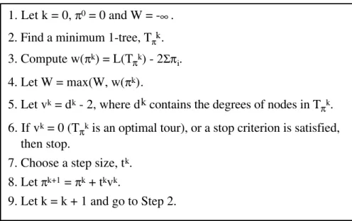
Figure 4.5 shows a subgradient algorithm for computing an approximation W for the maximum of w(π).
1. Let k = 0, π0 = 0 and W = -∞.
2. Find a minimum 1-tree, Tπk.
3. Compute w(πk) = L(T
πk) - 2Σπi.
4. Let W = max(W, w(πk).
5. Let vk = dk - 2, where dk contains the degrees of nodes in T
πk.
6. If vk = 0 (T
πk is an optimal tour), or a stop criterion is satisfied,
then stop.
7. Choose a step size, tk.
8. Let πk+1 = πk + tkvk.
9. Let k = k + 1 and go to Step 2.
Figure 4.5 Subgradient optimization algorithm.
It has been proven [26] that W will always converge to the maximum of w(π), if tk → 0 for k → ∞ and ∑tk = ∞. These conditions are satisfied, for
example, if tk is t0/k, where t0 is some arbitrary initial step size. But even if
convergence is guaranteed, it is very slow.
No general methods to determine an optimum strategy for the choice of step size are known. However, many strategies have been suggested that are quite effective in practice [25, 27, 28, 29, 30, 31]. These strategies are heuristics, and different variations have different effects on different problems. In the present implementation of the modified Lin-Kernighan algorithm the follow-ing strategy was chosen (inspired by [27] and [31]):
• The step size is constant for a fixed number of iterations, called a period. • When a period is finished, both the length of the period and the step size
are halved.
• The length of the first period is set to n/2, where n is the number of cities. • The initial step size, t0, is set to 1, but is doubled in the beginning of the
first period until W does not increase, i.e., w(πk) ≤ w(πk-1). When this
happens, the step size remains constant for the rest of the period.
• If the last iteration of a period leads to an increment of W, then the period is doubled.
• The algorithm terminates when either the step size, the length of the period or vk becomes zero.
Furthermore, the basic subgradient algorithm has been changed on two points (inspired by [13]):
• The updating of π, i.e., πk+1 = πk + tkvk, is replaced by
πk+1 = πk + tk(0.7vk + 0.3vk-1), where v-1 = v0.
• The special node for the 1-tree computations is not fixed. A minimum 1-tree is determined by computing a minimum spanning tree and then
adding an edge corresponding to the second nearest neighbor of one of the leaves of the tree. The leaf chosen is the one that has the longest second nearest neighbor distance.
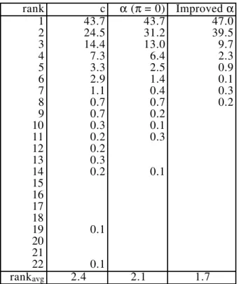
Table 4.1 shows the percent of optimal edges having a given rank among the nearest neighbors with respect to the c-measure, the α-measure, and the im-proved α-measure, respectively.
rank c α (π = 0) Improved α 1 43.7 43.7 47.0 2 24.5 31.2 39.5 3 14.4 13.0 9.7 4 7.3 6.4 2.3 5 3.3 2.5 0.9 6 2.9 1.4 0.1 7 1.1 0.4 0.3 8 0.7 0.7 0.2 9 0.7 0.2
10 0.3 0.1 11 0.2 0.3 12 0.2
13 0.3
14 0.2 0.1 15
16 17 18
19 0.1 20
21
22 0.1
rankavg 2.4 2.1 1.7
Table 4.1. The percentage of optimal edges among candi-date edges for the 532-city problem.
It appears from the table that the transformation of the cost matrix has the ef-fect that optimal edges come ‘nearer’, when measured by their α-values. The transformation of the cost matrix ‘conditions’ the problem, so to speak. Therefore, the transformed matrix is also used during the Lin-Kernighan search process. Most often the quality of the solutions is improved by this means.
The candidate edges of each node are sorted in ascending order of their α -val-ues. If two edges have the same α-value, the one with the smallest cost, cij, comes first. This ordering has the effect that candidate edges are considered for inclusion in a tour according to their ‘promise’ of belonging to an optimal tour. Thus, the α-measure is not only used to limit the search, but also to fo-cus the search on the most promising areas.
To speed up the search even more, the algorithm uses a dynamic ordering of the candidates. Each time a shorter tour is found, all edges shared by this new tour and the previous shortest tour become the first two candidate edges for their end nodes.
This method of selecting candidates was inspired by Stewart [32], who dem-onstrated how minimum spanning trees could be used to accelerate 3-opt heu-ristics. Even when subgradient optimization is not used, candidate sets based on minimum spanning trees usually produce better results than nearest neigh-bor candidate sets of the same size.
Johnson [17] in an alternative implementation of the Lin-Kernighan algorithm used precomputed candidate sets that usually contained more than 20 (ordi-nary) nearest neighbors of each node. The problem with this type of candidate set is that the candidate subgraph need not be connected even when a large fraction of all edges is included. This is, for example, the case for geometrical problems in which the point sets exhibit clusters. In contrast, a minimum spanning tree is (by definition) always connected.
Other candidate sets may be considered. An interesting candidate set can be obtained by exploiting the Delaunay graph [13, 33]. The Delaunay graph is connected and may be computed in linear time, on the average. A disadvan-tage of this approach, however, is that candidate sets can only be computed for geometric problem instances. In contrast, the α-measure is applicable in general.
4.2 Breaking of tour edges
A candidate set is used to prune the search for edges, Y, to be included in a tour. Correspondingly, the search of edges, X, to be excluded from a tour may be restricted. In the actual implementation the following simple, yet very effective, pruning rules are used:
(1) The first edge to be broken, x1, must not belong to the currently best
solution tour. When no solution tour is known, that is, during the determination of the very first solution tour, x1 must not belong to
The first rule prunes the search already at level 1 of the algorithm, whereas the original algorithm of Lin and Kernighan prunes at level 4 and higher, and only if an edge to be broken is a common edge of a number (2-5) of solution tours. Experiments have shown that the new pruning rule is more effective. In addition, it is easier to implement.
The second rule prevents an infinite chain of moves. The rule is a relaxation of Rule 4 in Section 3.2.
4.3 Basic moves
Central in the Lin-Kernighan algorithm is the specification of allowable moves, that is, which subset of r-opt moves to consider in the attempt to transform a tour into a shorter tour.
The original algorithm considers only r-opt moves that can be decomposed into a 2- or 3-opt move followed by a (possibly empty) sequence of 2-opt moves. Furthermore, the r-opt move must be sequential and feasible, that is, it must be a connected chain of edges where edges removed alternate with edges added, and the move must result in a feasible tour. Two minor devia-tions from this general scheme are allowed. Both have to do with 4-opt moves. First, in one special case the first move of a sequence may be a se-quential 4-opt move (see Figure 3.7); the following moves must still be 2-opt moves. Second, nonsequential 4-opt moves are tried when the tour can no longer be improved by sequential moves (see Figure 3.3).
The new modified Lin-Kernighan algorithm revises this basic search structure on several points.
First and foremost, the basic move is now a sequential 5-opt move. Thus, the moves considered by the algorithm are sequences of one or more 5-opt moves. However, the construction of a move is stopped immediately if it is discovered that a close up of the tour results in a tour improvement. In this way the algorithm attempts to ensure 2-, 3-, 4- as well as 5-optimality.
The new algorithm’s improved performance compared with the original algo-rithm is in accordance with observations made by Christofides and Eilon [16]. They observed that 5-optimality should be expected to yield a relatively superior improvement over 4-optimality compared with the improvement of 4-optimality over 3-optimality.
Another deviation from the original algorithm is found in the examination of nonsequential exchanges. In order to provide a better defense against possible improvements consisting of nonsequential exchanges, the simple nonsequen-tial 4-opt move of the original algorithm has been replaced by a more power-ful set of nonsequential moves.
This set consists of
• any nonfeasible 2-opt move (producing two cycles) followed by any 2- or 3-opt move, which produces a feasible tour (by joining the two
cycles);
• any nonfeasible 3-opt move (producing two cycles) followed by any 2-opt move, which produces a feasible tour (by joining the two cycles). As seen, the simple nonsequential 4-opt move of the original algorithm be-longs to this extended set of nonsequential moves. However, by using this set of moves, the chances of finding optimal tours are improved. By using candidate sets and the “positive gain criterion” the time for the search for such nonsequential improvements of the tour is small relative to the total running time.
Unlike the original algorithm the search for nonsequential improvements is not only seen as a post optimization maneuver. That is, if an improvement is found, further attempts are made to improve the tour by ordinary sequential as well as nonsequential exchanges.
4.4 Initial tours
The Lin-Kernighan algorithm applies edge exchanges several times to the same problem using different initial tours.
In the original algorithm the initial tours are chosen at random. Lin and Ker-nighan concluded that the use of a construction heuristic only wastes time. Besides, construction heuristics are usually deterministic, so it may not be possible to get more than one solution.
Clarke and Wright savings heuristic [36] in general improved the performance of the algorithm. Reinelt [13] also found that is better not to start with a ran-dom tour. He proposed using locally good tours containing some major er-rors, for example the heuristics of Christofides [37]. However, he also ob-served that the difference in performance decreases with more elaborate ver-sions of the Lin-Kernighan algorithm.
Experiments with various implementations of the new modified Lin-Ker-nighan algorithm have shown that the quality of the final solutions does not depend strongly on the initial tours. However, significant reduction in run time may be achieved by choosing initial tours that are close to being optimal. In the present implementation the following simple construction heuristic is used:
1. Choose a random node i.
2. Choose a node j, not chosen before, as follows: If possible, choose j such that
(a) (i,j) is a candidate edge, (b) α(i,j) = 0, and
(c) (i,j) belongs to the current best tour.
Otherwise, if possible, choose j such that (i,j) is a candidate edge. Otherwise, choose j among those nodes not already chosen. 3. Let i = j. If not all nodes have been chosen, then go to Step 2.
If more than one node may be chosen at Step 2, the node is chosen at random among the alternatives. The sequence of chosen nodes constitutes the initial tour.
This construction procedure is fast, and the diversity of initial solutions is large enough for the edge exchange heuristics to find good final solutions. 4.5 Specification of the modified algorithm
Below is given a sketch of the main program.
void main() {
ReadProblemData(); CreateCandidateSet(); BestCost = DBL_MAX;
for (Run = 1; Run <= Runs; Run++) { double Cost = FindTour();
if (Cost < BestCost) { RecordBestTour(); BestCost = Cost;
} }
PrintBestTour(); }
First, the program reads the specification of the problem to be solved and cre-ates the candidate set. Then a specified number (Runs) of local optimal tours is found using the modified Lin-Kernighan heuristics. The best of these tours is printed before the program terminates.
The creation of the candidate set is based on α-nearness.
void CreateCandidateSet() {
double LowerBound = Ascent();
long MaxAlpha = Excess * fabs(LowerBound); GenerateCandidates(MaxCandidates, MaxAlpha); }
First, the function Ascent determines a lower bound on the optimal tour length using subgradient optimization. The function also transforms the origi-nal problem into a problem in which α-values reflect the likelihood of edges being optimal. Next, the function GenerateCandidates computes the α -val-ues and associates to each node a set of incident candidate edges. The edges are ranked according to their α-values. The parameter MaxCandidates speci-fies the maximum number of candidate edges allowed for each node, and MaxAlpha puts an upper limit on their α-values. The value of MaxAlpha is set to some fraction, Excess, of the lower bound.
double Ascent() { Node *N;
double BestW, W;
int Period = InitialPeriod, P, InitialPhase = 1;
W = Minimum1TreeCost(); if (Norm == 0) return W;
GenerateCandidates(AscentCandidates, LONG_MAX); BestW = W;
ForAllNodes(N) {
N->LastV = N->V; N->BestPi = N->Pi; }
for (T = InitialStepSize; T > 0; Period /= 2, T /= 2) { for (P = 1; T > 0 && P <= Period; P++) {
ForAllNodes(N) {
if (N->V != 0)
N->Pi += T*(7*N->V + 3*N->LastV)/10; N->LastV = N->V;
}
W = Minimum1TreeCost(); if (Norm == 0) return W; if (W > BestW) {
BestW = W; ForAllNodes(N)
N->BestPi = N->Pi; if (InitialPhase) T *= 2; if (P == Period) Period *= 2; }
else if (InitialPhase && P > InitalPeriod/2) { InitialPhase = 0;
P = 0; T = 3*T/4; }
} }
ForAllNodes(N)
Below is shown the pseudo code of the function GenerateCandidates. For each node at most MaxCandidates candidate edges are determined. This up-per limit, however, may be exceeded if a “symmetric” neighborhood is de-sired (SymmetricCandidates != 0) in which case the candidate set is com-plemented such that every candidate edge is associated to both its two end nodes.
void GenerateCandidates(long MaxCandidates, long MaxAlpha) { Node *From, *To;
long Alpha; Candidate *Edge;
ForAllNodes(From)
From->Mark = 0;
ForAllNodes(From) {
if (From != FirstNode) { From->Beta = LONG_MIN;
for (To = From; To->Dad != 0; To = To->Dad) { To->Dad->Beta = max(To->Beta, To->Cost); To->Dad->Mark = From;
} }
ForAllNodes(To, To != From) {
if (From == FirstNode)
Alpha = To == From->Father ? 0 : C(From,To) - From->NextCost;
else if (To == FirstNode)
Alpha = From == To->Father ? 0: C(From,To) - To->NextCost; else {
if (To->Mark != From)
To->Beta = max(To->Dad->Beta, To->Cost); Alpha = C(From,To) - To->Beta;
}
if (Alpha <= MaxAlpha)
InsertCandidate(To, From->CandidateSet);
} }
if (SymmetricCandidates)
ForAllNodes(From)
ForAllCandidates(To, From->CandidateSet)
if (!IsMember(From, To->CandidateSet))
InsertCandidate(From, To->CandidateSet);
After the candidate set has been created the function FindTour is called a pre-determined number of times (Runs). FindTour performs a number of trials where in each trial it attempts to improve a chosen initial tour using the modi-fied Lin-Kernighan edge exchange heuristics. Each time a better tour is found, the tour is recorded, and the candidates are reordered with the function AdjustCandidateSet. Precedence is given to edges that are common to the two currently best tours. The candidate set is extended with those tour edges that are not present in the current set. The original candidate set is re-estab-lished at exit from FindTour.
double FindTour() { int Trial;
double BetterCost = DBL_MAX, Cost;
for (Trial = 1; Trial <= Trials; Trial++) { ChooseInitialTour();
Cost = LinKernighan(); if (Cost < BetterCost) { RecordBetterTour(); BetterCost = Cost AdjustCandidateSet(); }
}
ResetCandidateSet(); return BetterCost; }
double LinKernighan() { Node *t1, *t2; int X2, Failures; long G, Gain; double Cost = 0;
ForAllNodes(t1)
Cost += C(t1,SUC(t1)); do {
Failures = 0;
ForallNodes(t1, Failures < Dimension) {
for (X2 = 1; X2 <= 2; X2++) {
t2 = X2 == 1 ? PRED(t1) : SUC(t1); if (InBetterTour(t1,t2))
continue; G = C(t1,t2);
while (t2 = BestMove(t1, t2, &G, &Gain)) { if (Gain > 0) {
Cost -= Gain; StoreTour(); Failures = 0; goto Next_t1; }
}
Failures++; RestoreTour(); }
Next_t1: ; }
if ((Gain = Gain23()) > 0) { Cost -= Gain;
StoreTour(); }
} while (Gain > 0); }
The function BestMove is sketched below. The function BestMove makes sequential edge exchanges. If possible, it makes an r-opt move (r ≤ 5) that improves the tour. Otherwise, it makes the most promising 5-opt move that fulfils the positive gain criterion.
Node *BestMove(Node *t1, Node *t2, long *G0, long *Gain) { Node *t3, *t4, *t5, *t6, *t7, *t8, *t9, *t10;
Node *T3, *T4, *T5, *T6, *T7, *T8, *T9, *T10 = 0;
long G1, G2, G3, G4, G5, G6, G7, G8, BestG8 = LONG_MIN; int X4, X6, X8, X10;
*Gain = 0; Reversed = SUC(t1) != t2;
ForAllCandidates(t3, t2->CandidateSet) {
if (t3 == PRED(t2) || t3 == SUC(t2) || (G1 = *G0 - C(t2,t3)) <= 0)
continue;
for (X4 = 1; X4 <= 2; X4++) {
t4 = X4 == 1 ? PRED(t3) : SUC(t3); G2 = G1 + C(t3,t4);
if (X4 == 1 && (*Gain = G2 - C(t4,t1)) > 0) { Make2OptMove(t1, t2, t3, t4);
return t4; }
ForAllCandidates(t5, t4->CandidateSet) {
if (t5 == PRED(t4) || t5 == SUC(t4) || (G3 = G2 - C(t4,t5)) <= 0)
continue;
for (X6 = 1; X6 <= 2; X6++) {
Determine (T3,T4,T5,T6,T7,T8,T9,T10) =
(t3,t4,t5,t6,t7,t8,t9,t10) such that
G8 = *G0 - C(t2,T3) + C(T3,T4)
- C(T4,T5) + C(T5,T6) - C(T6,T7) + C(T7,T8) - C(T8,T9) + C(T9,T10) is maximum (= BestG8), and (T9,T10) has not previously been included; if during
this process a legal move with *Gain > 0
is found, then make the move and exit
from BestMove immediately;
} } } }
*Gain = 0;
if (T10 == 0) return 0;
Make5OptMove(t1,t2,T3,T4,T5,T6,T7,T8,T9,T10); *G0 = BestG8;
Only the first part of the function (the 2-opt part) is given in some detail. The rest of the function follows the same pattern. The tour is as a circular list. The flag Reversed is used to indicate the reversal of a tour.
To prevent an infinite chain of moves the last edge to be deleted in a 5-opt move, (T9,T10), must not previously have been included in the chain.
5. Implementation
The modified Lin-Kernighan algorithm has been implemented in the pro-gramming language C. The software, approximately 4000 lines of code, is entirely written in ANSI C and portable across a number of computer plat-forms and C compilers. The following subsections describe the user interface and the most central techniques employed in the implementation.
5.1 User interface
The software includes code both for reading problem instances and for print-ing solutions.
Input is given in two separate files: (1) the problem file and (2) the parameter file.
The problem file contains a specification of the problem instance to be solved. The file format is the same as used in TSPLIB [38], a publicly available library of problem instances of the TSP.
The current version of the software allows specification of symmetric, asym-metric, as well as Hamiltonian tour problems.
Distances (costs, weights) may be given either explicitly in matrix form (in a full or triangular matrix), or implicitly by associating a 2- or 3-dimensional coordinate with each node. In the latter case distances may be computed by either a Euclidean, Manhattan, maximum, geographical or pseudo-Euclidean distance function. See [38] for details. At present, all distances must be inte-gral.
The format is as follows:
PROBLEM_FILE = <string>
Specifies the name of the problem file.
Additional control information may be supplied in the following format:
RUNS = <integer> The total number of runs. Default: 10.
MAX_TRIALS = <integer>
The maximum number of trials in each run.
Default: number of nodes (DIMENSION, given in the problem file).
TOUR_FILE = <string>
Specifies the name of a file to which the best tour is to be written.
OPTIMUM = <real>
Known optimal tour length. A run will be terminated as soon as a tour length less than or equal to optimum is achieved.
Default: DBL_MAX.
MAX_CANDIDATES = <integer> { SYMMETRIC }
The maximum number of candidate edges to be associated with each node. The integer may be followed by the keyword SYMMETRIC, signifying that the candidate set is to be complemented such that every candidate edge is associated with both its two end nodes.
Default: 5.
ASCENT_CANDIDATES = <integer>
The number of candidate edges to be associated with each node during the ascent. The candidate set is complemented such that every candidate edge is associated with both its two end nodes.
Default: 50.
EXCESS = <integer>
The maximum α-value allowed for any candidate edge is set to EXCESS times the absolute value of the lower bound of a solution tour (determined by the ascent). Default: 1.0/DIMENSION.
INITIAL_PERIOD = <integer>
The length of the first period in the ascent. Default: DIMENSION/2 (but at least 100).
PI_FILE = <string>
Specifies the name of a file to which penalties (π-values determined by the ascent) is to be written. If the file already exits, the penalties are read from the file, and the ascent is skipped.
PRECISION = <integer>
The internal precision in the representation of transformed distances: dij = PRECISION*cij + πi + πj, where dij, cij, πi and πj are all integral. Default: 100 (which corresponds to 2 decimal places).
SEED = <integer>
Specifies the initial seed for random number generation. Default: 1.
SUBGRADIENT: [ YES | NO ]
Specifies whether the π-values should be determined by subgradient optimization. Default: YES.
TRACE_LEVEL = <integer>
Specifies the level of detail of the output given during the solution process. The value 0 signifies a minimum amount of output. The higher the value is the more information is given.
Default: 1.
During the solution process information about the progress being made is written to standard output. The user may control the level of detail of this in-formation (by the value of the TRACE_LEVEL parameter).
Before the program terminates, a summary of key statistics is written to stan-dard output, and, if specified by the TOUR_FILE parameter, the best tour found is written to a file (in TSPLIB format).
The user interface is somewhat primitive, but it is convenient for many appli-cations. It is simple and requires no programming in C by the user. However, the current implementation is modular, and an alternative user interface may be implemented by rewriting a few modules. A new user interface might, for example, enable graphical animation of the solution process.
5.2 Representation of tours and moves
The data structure should support the following primitive operations: (1) find the predecessor of a node in the tour with respect to a chosen orientation (PRED);
(2) find the successor of a node in the tour with respect to a chosen orientation (SUC);
(3) determine whether a given node is between two other nodes in the tour with respect to a chosen orientation (BETWEEN); (4) make a move;
(5) undo a sequence of tentative moves.
The necessity of the first three operations stems from the need to determine whether it is possible to 'close' the tour (see Figures 3.5-3.7). The last two operations are necessary for keeping the tour up to date.
In the modified Lin-Kernighan algorithm a move consists of a sequence of basic moves, where each basic move is a 5-opt move (k-opt moves with k ≤ 4 are made in case an improvement of the tour is possible).
In order simplify tour updating, the following fact may be used: Any r-opt move (r ≥ 2) is equivalent to a finite sequence of 2-opt moves [16, 39]. In the case of 5-opt moves it can be shown that any 5-opt move is equivalent to a sequence of at most five 2-opt moves. Any 4-opt move as well as any 3-opt move is equivalent to a sequence of at most three 2-opt moves.
This is exploited as follows. Any move is executed as a sequence of one or more 2-opt moves. During move execution, all 2-opt moves are recorded in a stack. A bad move is undone by unstacking the 2-opt moves and making the inverse 2-opt moves in this reversed sequence.
Thus, efficient execution of 2-opt moves is needed. A 2-opt move, also called a swap, consists of moving two edges from the current tour and reconnecting the resulting two paths in the best possible way (see Figure 2.1). This opera-tion is seen to reverse one of the two paths. If the tour is represented as an array of nodes, or as a doubly linked list of nodes, the reversal of the path takes time O(n).
outperformed by update algorithms based on the array and list structures. In addition, they are not simple to implement.
In the current implementation of the modified Lin-Kernighan algorithm a tour may be represented in two ways, either by a doubly linked list, or by a two-level tree [43]. The user can select one of these two representations. The dou-bly linked list is recommended for problems with fewer than 1000 nodes. For larger problems the two-level tree should be chosen.
When the doubly link list representation is used, each node of the problem is represented by a C structure as outlined below.
struct Node {
unsigned long Id, Rank; struct Node *Pred, *Suc; };
The variable Id is the identification number of the node (1 ≤ Id ≤ n).
Rank gives the ordinal number of the node in the tour. It is used to quickly determine whether a given node is between two other nodes in the tour. Pred and Suc point to the predecessor node and the successor node of the tour, respectively.
A 2-opt move is made by swapping Pred and Suc of each node of one of the two segments, and then reconnecting the segments by suitable settings of Pred and Suc of the segments’ four end nodes. In addition, Rank is updated for nodes in the reversed segment.
The following small code fragment shows the implementation of a 2-opt move. Edges (t1,t2) and (t3,t4) are exchanged with edges (t2,t3) and (t1,t4) (see Figure 3.1).
R = t2->Rank; t2->Suc = 0; s2 = t4; while (s1 = s2) {
s2 = s1->Suc;
s1->Suc = s1->Pred; s1->Pred = s2; s1->Rank = R--; }
Any of the two segments defined by the 2-opt move may be reversed. The segment with the fewest number of nodes is therefore reversed in order to speed up computations. The number of nodes in a segment can be found in constant time from the Rank-values of its end nodes. In this way much run time can be spared. For an example problem with 1000 nodes the average number of nodes touched during reversal was about 50, whereas a random reversal would have touched 500 nodes, on the average. For random Euclid-ean instances, the length of the shorter segment seems to grow roughly as n0.7
[44].
However, the worst-case time cost of a 2-opt move is still O(n), and the costs of tour manipulation grow to dominate overall running time as n increases. A worst-case cost of O(√n) per 2-opt move may be achieved using a two-level tree representation. This is currently the fastest and most robust representation on large instances that might arise in practice. The idea is to divide the tour into roughly √n segments. Each segment is maintained as a doubly linked list of nodes (using pointers labeled Pred and Suc).
Each node is represented by a C structure as outlined below.
struct Node {
unsigned long Id, Rank; struct Node *Pred, *Suc; struct Segment *Parent; };
Rank gives the position of the node within the segment, so as to facilitate BETWEEN queries. Parent is a pointer the segment containing the node. Each segment is represented by the following C structure.
struct Segment {
unsigned long Rank;
struct Segment *Pred, *Suc; struct Node *First, *Last; bit Reversed;
};