101 The European Journal of Management
Studies is a publication of ISEG, Universidade de Lisboa. The mission of EJMS is to significantly influence the domain of management studies by publishing innovative research articles. EJMS aspires to provide a platform for thought leadership and outreach.
Editors-in-Chief: Luís M. de Castro, PhD
ISEG - Lisbon School of Economics and Management, Universidade de Lisboa, Portugal
Gurpreet Dhillon, PhD
Virginia Commonwealth University, USA Tiago Cardão-Pito, PhD
ISEG - Lisbon School of Economics and Management, Universidade de Lisboa, Portugal
Managing Editor: Mark Crathorne, MA
ISEG - Lisbon School of Economics and Management, Universidade de Lisboa, Portugal
ISSN: 2183-4172 Volume 21, Issue 2
www.european-jms.com
WHAT DRIVES FOREIGN DIRECT
INVESTMENT IN THE TRADABLE
SECTOR?
Márcio Mateus1, Isabel Proença2, and Paulo Júlio3
1Banco de Portugal, Financial Stability Department, Portugal; 2ISEG – Lisbon School of Economics and Management, Universidade de Lisboa, and CEMAPRE, Portugal; 3Banco de Portugal, Economics and Research Department, and CEFAGE, Portugal.
Abstract
Researchers usually investigate the determinants of aggregated Foreign Direct Investment (FDI), although there is evidence that the sectoral distribution of FDI matters and that too much FDI in the non-tradable sector can exacerbate external imbalances. This paper differs from most existing studies on FDI determinants by focusing on tradable sector FDI. We show that countries with a large market size, a higher degree of economic openness, a higher productivity level and good institutions are more likely to receive FDI in the tradable sector. We also show that physical distance does not represent so large an obstacle for tradable sector FDI, as it seems to represent for aggregated FDI. In contrast, based on results of empirical studies on aggregated FDI which share a common border, it does not seem to have an impact on the attraction of FDI for the tradable sector. This paper uses a modified gravity model to compare different methods, specifications and variables, in order to obtain robust results1.
Key words: Gravity models, Econometrics, Foreign Direct Investment, European Union.
1 The authors would like to acknowledge the following financial support: Isabel Proença - FCT (Fundação
102
Introduction
One important feature of globalisation has been the significant increase in the flows of people, goods, services and investment between countries. According to the United Nations Conference on Trade and Development (UNCTAD)2, from 1990 to 2013, Foreign Direct Investment (FDI) stocks have grown by a factor of more than 12. Over the same period of time, by comparison, the world Gross Domestic Product (GDP) has only grown by a factor of approximately 3.3, and global exports of goods and services have grown by a factor of nearly 5.6. In 2007, prior to the financial crisis, developed countries hosted nearly 71 percent of the world’s FDI positions, 42 percent targeted to the European Union. Since then, the share of developed countries in the world’s inward FDI has decreased to 63 percent, due to the decline of the FDI hosted by European Union countries (-8 percent to 34 percent). This evolution, explained by the economic and financial turmoil in Europe, urges the European Union to design successful policies to attract FDI investors.
Over the last decades, as multinational firms increasingly seek to spread their production all over the world in order to exploit countries’ comparative advantages, the attraction of FDI has acquired a significant importance for both developing and developed economies. The attraction of FDI has become a key issue, as this type of investment, when compared with other types, generally has a more significant impact on long-run growth and development (Barrell and Pain, 1996; Borensztein et al., 1998). In fact, a direct investment relationship involves control, or a significant degree of influence on the management from the investor to the investee, which means that it tends to involve a lasting relationship between companies and countries.
The literature shows that both investor and host countries benefit from FDI. For host countries, FDI means investment, job creation, technological transfer, improvement of managerial and marketing skills, an increase in productivity, and improvement of the host country’s institutions (Larraín and Tavares, 2004). FDI can also contribute to correct external imbalances, as multinational firms have a greater propensity to export than domestic firms usually have. For investor countries and companies, this kind of investment can also be positive. Investor companies can spread their production all over the world to take advantage of countries’ specific comparative advantages (natural resources, less expensive or more qualified labour, legal framework, etc.). They can also reduce their risk by diversifying their holdings outside a specific country. For the investor country, FDI could also improve the access to foreign markets and lead to increase exports.
The vast majority of researchers investigate the determinants of aggregate FDI, which is an approach that can lead to spurious conclusions about what a country can do to attract FDI, as aggregated FDI can be inflated by the presence of Special Purpose Entities (SPEs). These kind of entities choose their geographical location for tax reasons, have significant positions in direct investment (inward and outward), and a very small number of workers. More importantly, they do not carry out substantial real economic activity in the countries where they are located.
103 Additionally, investments in other economic activities (agriculture, mining, manufacturing, real estate, education, wholesale and retail trade, etc.) come under the umbrella of FDI. Buying a stake in a monopolist company operating in a protected economic sector is as much FDI as is investing in a company operating in a sector open to external competition. These two types of investment could have a very different impact on the host country’s economy. This study differs from existing studies on FDI determinants as it focuses on tradable sector FDI, instead of aggregate FDI.
Kinoshita (2011) studies the sectoral composition of FDI in Eastern Europe and finds that FDI in the non-tradable sector can exacerbate external imbalances of countries, while FDI in the tradable sectors leads to an improvement of the external balance. FDI in the tradable sector is expected to increase exports over time3, while FDI in the non-tradable sector may fuel domestic demand and boost imports. Thus, according to Kinoshita (2011), countries where FDI is mainly targeted to the non-tradable sector are expected to present a higher trade deficit than countries where FDI is mainly targeted to the tradable sector. In this sense, the question policy makers should focus on is not how to attract FDI, but instead how to attract tradable sector FDI. This is especially important for those European countries with significant external imbalances.4 Data seems to support the idea that FDI in the tradable sector is associated with higher exports (see Figure B.1 in the Appendix) and current and capital account surpluses (see Figure B.2 and B.3 in the Appendix). This paper will therefore focus on tradable sector FDI, as this is more open to international competition, with more potential to export and to create jobs and to transfer know-how. More importantly, it can be an important tool to solve external imbalances of countries.
As a proxy for the tradable sector we use the manufacturing sector.5 This sector does not usually contain SPE’s, allowing us to avoid their effect.
In this paper we first examine the role of economic, geographic, and institutional variables in attracting tradable sector FDI to European Union countries. We demonstrate that a large market size, a higher degree of economic openness, a higher productivity level and good institutions are all key driving forces of tradable sector FDI. We then compare our results for tradable sector FDI with those obtained in the literature for aggregated FDI. We show that physical distance does not represent an obstacle that is impossible to overcome for tradable sector FDI, as it seems to represent for aggregated FDI. Finally, we also demonstrate that the degree of economic openness is much more important as a tradable sector FDI determinant, than as an aggregated FDI determinant.
3 Tradable sector FDI can also imply a reduction of imports once imported goods are replaced by
domestically-produced goods.
4 The Eurozone debt crisis was a typical balance of payments crisis (Higgins and Klitgaard, 2014), and some of
the most affected countries (Greece, Spain and Portugal) also presented the highest external imbalances (see Figure B.2 in the Appendix).
104
Throughout this paper we compare the performance of different methods, specifications and variables in the estimation of a gravity model and find out the best way to deal with zero-FDI values, heteroscedasticity, and heterogeneity across countries. We will apply a modified gravity model, using both a cross-section and a panel data specification.
The remainder of this paper is organized in the following way. Section 2 reviews the economic and econometric literature. The next section presents the data used in the empirical analysis. Section 4 presents the econometric methodology, and Section 5 presents the results obtained. Section 6 concludes.
Literature Review
Economic and econometric literature
The FDI literature initially focused on economic and geographical determinants, including host-country market size, economic growth, economic openness, labour costs, tax rates and geographical distance between countries. Market size, measured as the GDP level or population, is the economic determinant that receives most attention in the literature. Billington (1999), Scaperlanda and Balough (1983) and Júlio et al. (2013) find a statistically significant impact of market size and growth on FDI. Barrel and Pain (1996) also find a link between market size and FDI. Culem (1988) and Kinoshita (2011) conclude that a greater degree of openness affects aggregate FDI and the tradable sector FDI in a positive way, respectively. Barrel and Pain (1996) and Culem (1988) find a negative impact for labour costs on FDI, while Tsai (1994), Wheeler and Mody (1992), Kravis and Lipsey (1982) find a non-statistically significant or positive effect. Hartman (1984, 1985) and Cassou (1997) find a negative relationship between taxation and FDI. Altomonte and Guagliano (2003) find that education has a negative effect on the investment of multinational companies in Central and Eastern Europe countries, while for investment in the Mediterranean countries they find a positive effect of education on investment targeted to the services sector and a negative effect on investment targeted to traditional industries. Kinoshita (2011), also for a panel of Eastern Europe countries, finds that a highly educated labour force positively affects the share of FDI in the tradable sector. The distance between countries (Júlio et al., 2013), or the distance to a central city (Altomonte and Guagliano, 2003 and Kinoshita, 2011) is used in literature as a proxy of the physical and cultural barriers, and also as a proxy of transaction costs.6 Sometimes it is also used as a proxy for the ease of access to a major consumer market. Either way, authors find a negative effect of distance on FDI.
Over the last years, a second wave of research articles have pointed out that institutional and political factors play also a role in explaining inward FDI. As transaction costs were reduced with
6 The impact of transaction costs in FDI is not as obvious as it is in trade, but they still exist, as distance
105 the proliferation of intra-regional integration agreements, competition between countries in attracting FDI started to be based on business facilitation measures that provide investing firms a better business environment. According to Stein and Daude (2007), the impact of institutions on investment can be reflected through two different channel. First, bad institutions increase the cost of doing business. Second, poor enforcement of contracts is expected to increase the uncertainty associated with future returns, and thus has a negative impact on investment. The classical example of bad institutions is corruption, which represents increased cost of doing business and uncertainty.
Schneider and Frey (1985) were among the pioneers in assessing the importance of institutional factors, and they show a negative relationship between political instability and inward investment.
Biswas (2002) concludes that institutions are important determinants of FDI inflows. Wei (2000) and Wei and Shleifer (2000) show that corruption has a negative impact on inward FDI. Lee and Mansfield (1996) and Knack and Keefer (1995) conclude that FDI inflows are positively correlated with the protection of property rights and intellectual property. Several other studies also report that FDI is positively associated with the efficiency of the legal system (Buch et al., 2005), with the regulation of labour markets (Botero et al., 2004) and investors’ protection (Djankov et al., 2008).
While a substantial amount of research has been devoted to study aggregated FDI, very few authors have devoted their time to analyse sectoral FDI, in part due to the unavailability of this kind of data.7 Altomonte and Guagliano (2003) constructed a panel of European multinationals that have invested in Central and Eastern Europe and in the Mediterranean (in 48 NACE 3 industries) and find that education matters for FDI targeted to the services sector, but not to FDI targeted to traditional industries. Zhang (2005), using disaggregated industry level data, finds that FDI hosted by China has a stronger effect on exports from labour-intensive sectors than from capital-intensive industries. Kinoshita (2011) studies the sectoral composition of FDI in Eastern Europe and finds that tradable sector FDI leads to an improvement of the external balance, while investment in the non-tradable sector has the opposite effect.
A significant amount of the trade and FDI literature has been developed based on gravity models over the last decades. Gravity models were first introduced by Tinbergen (1962) in the context of international trade, based on the idea that a gravity relationship, analogous to the Newton’s law of universal gravitation, can explain trade flows between countries.8 In its simplest formulation, the gravity model for international trade states that bilateral trade between country i to country j is proportional to the product of the two countries GDPs, and that it is inversely proportional to
7 Industry-specific information on bilateral FDI position is not available in official statistics, even for some
European countries, therefore researchers sometimes use firm-level data on multinational enterprises available on commercial databases.
8 Newton’s law of universal gravitation states that any two bodies in the universe attract each other with a
106
their physical distance. Ever since the first successful application to trade, gravity models have also been used to model tourism, migration and bilateral FDI.
The usual procedure of the FDI literature consists in estimating the multiplicative gravity equation, after the model is log-linearly transformed, applying the traditional ordinary least squares technique (OLS). Santos Silva & Tenreyro (2006), using cross-sectional data, showed that, in the presence of heteroscedasticity in the multiplicative error, the consistent estimation of the gravity equation by OLS after the logarithmic transformation entails very strong assumptions that do not hold in general. Moreover, due to the Jensen’s inequality, which states that the expected value of the logarithm of a random variable is not equal to the logarithm of its expected value, logarithmic transformed models can be significantly misleading in estimating elasticities and semi-elasticities. The consistent estimation of the log-linearized model relies critically on the assumption that the error term, and also the log of the error term, are statistically independent of the regressors. However, the expected value of the logarithm of a random variable depends, in general, both on the mean and on higher-order moments of the distribution. For example, if the variance of the error term 𝜑𝑖𝑗 depends on regressors, the expected value of ln(𝜑𝑖𝑗) will also depend on regressors, and therefore OLS estimates will be inconsistent.
Santos Silva & Tenreyro (2006) illustrate this problem, considering the case in which ϕij follows a
log normal distribution, with E(𝜑𝑖𝑗| 𝐱𝑖𝑗) = 1 and variance 𝜎𝑖𝑗2 = 𝑓(𝐱𝑖𝑗), where 𝐱𝑖𝑗 is the vector containing the regressors. In the log-linearized specification the error term will follow a normal
distribution, with 𝐸(ln(𝜑𝑖𝑗) |𝐱𝑖𝑗) = −1
2ln(1 + 𝜎𝑖𝑗2) also a function of the covariates 𝐱𝑖𝑗. This way, Santos Silva & Tenreyro (2006) argue that in the presence of heteroscedasticity, the log-linearized errors will depend on the regressors, which leads to inconsistent estimates of OLS. The authors find strong evidence of the presence of heteroscedasticity in the empirical applications of the gravity model to the international trade analysed in their research.
Another problem concerning the log-linear transformation of the gravity equation is the existence of zeros (because the logarithm of zero is not defined). The usual approach followed in empirical studies to deal with this problem is simply to drop the pairs with zero values. Another alternative approach consists in adding 1 to the dependent variable observations. Santos Silva & Tenreyro (2006) conclude that is not advisable to follow these procedures and estimate the gravity equation in the log-linear form with OLS. They suggest estimating the gravity equation, and constant-elasticity models, in the multiplicative form, through a Poisson pseudo-maximum-likelihood (PPML) estimator. To assess the performance of this estimator, the authors performed a simulation study using different estimators (e.g. OLS, Tobit, NLS and PPML) and different patterns of heteroscedasticity. Results confirm that the PPML estimator is more robust than the alternatives.
107 results (Cheng and Wall (2005); Cheng and Tsai (2008). Panel data is an alternative that can mitigate this problem, allowing different types of heterogeneity to be taken into consideration.
The usual approach used to estimate the gravity model using panel data is to estimate the log-linearized version of the gravity equation by fixed effect least squares. Following Santos Silva & Tenreyro’s (2006) research with cross-sectional data, Westerlund & Wilhelmsson (2009) pointed out that the log-linearised model still causes problems with using panel data estimation methods. Zeros and the presence of heteroscedasticity also affect panel data usual estimators. The log-linearised gravity equations can only be estimated consistently by a least squares estimator if the conditional expected value of logarithm of the error term of the model equals zero. Following the arguments of Santos Silva & Tenreyro (2006), they stress that this assumption is violated with panel data as well, and, as a result, the fixed effects OLS estimator will be inconsistent.
Westerlund & Wilhelmsson (2009) also recommend to estimate gravity equations in their multiplicative form, and they propose a fixed effect Poisson pseudo-maximum-likelihood (FE-PPML) estimator. The authors compare the performance of OLS fixed effects estimator and PPML fixed effects on a simulation study, and conclude that OLS performed poorly when compared with PPML fixed effects. PPML estimation presented very small bias and good accuracy. Finally, Westerlund & Wilhelmsson (2009) argue that the PPML random effects estimator should not be used, as it assumes non-correlation of the individual specific effect with the other regressors, which is hard to verify in practice for many applications.
Proença et al. (2014) propose a semiparametric gravity model for panel data to overcome the above-mentioned problems. These authors introduce a non-parametric component in the gravity panel equation in order to capture the dependency between the explanatories and the unobserved individual heterogeneity term. The method proposed seeks to captures country unobserved heterogeneity that is dependent on the explanatories, without compromising the estimate of time-invariant variables and untransformed non-linear gravity equations.
Empirical results
108
literature are quite different from the one we are going to use, which makes it difficult and unwise to perform any comparison of results.
From the survey we carried out, five important conclusions emerge. First, host country GDP elasticity varies between 0.83 (Bénassy-Quéré et al., 2007) and 1.18 (Júlio et al., 2013), which means that estimates are usually around the unit. Second, estimated elasticities we found for distance between countries oscillate between -1.9 (Stein and Daude, 2007a) and -0.49 (Bénassy-Quéré et al., 2007). Nevertheless, the elasticity obtained by Stein and Daude (2007a) is clearly an outlier. Results usually obtained by authors vary between -0.9 and -0.49. Third, the contiguity dummy estimated coefficient varies between 0.55 (Júlio et al., 2013) and 2.5 (Stein and Daude, 2007b). As a general rule, the contiguity dummy comes out with a positive and statistically significant sign. Notwithstanding, studies exist which show a non-significant (Tong, 2005), or even a negative impact (Stein and Daude, 2007a) of sharing a common border. Fourth, the estimated coefficients we found in the literature for the degree of openness are relatively close, but are not always statistically significant. Júlio et al. (2013) estimates varies between 0.003 and 0.021, while Ali (2010) coefficients oscillate between 0.006 and 0.010. Fifth, the other variables do not appear so frequently as the previous ones, and the results are not entirely conclusive regarding the statistical significance and, sometimes, even regarding the signal of the estimated coefficient.
The results obtained by Júlio et al. (2013) with cross-sectional data demonstrate the huge importance of geographical determinants for aggregated FDI. According to these authors’ results, the investment of a country in its neighbour is between 73 and 88 percent higher than the investment in a similar country that does not share a common border. Physical distance is also a key determinant, as an increase of 1 percent in the number of kilometers between countries is expected to reduce aggregated FDI between 0.54 and 0.63 percent. Results also suggest that market size, economic growth and the quality of the host country’s institutions play an important role in the attraction of aggregated FDI.
The model and the variables used by Júlio et al. (2013) for aggregated FDI are quite similar to those we use for tradable sector FDI. The main differences between our research, and that of Júlio et al. (2013) is obviously the depend variable used. We use tradable sector FDI, while Júlio et al. (2013) use aggregated FDI. Additionally, the institutional variables used, the time span analysed, and the sample of source and host countries are not quite the same. Finally, Júlio et al. (2013) only use cross-section specification, while we use both cross-section and panel data. Thus, whenever we compare our results with the literature we are now going to rely mostly on Júlio et al.’s (2013) results as a reference. Even so, any comparison with Júlio et al. (2013) or other results should be looked at with caution, as different time periods or/and different sample of countries were used.
Data and variables
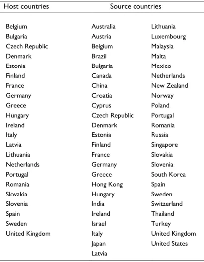
109 to the new European classification of economic activity NACE Rev. 2. The dataset covers FDI from 47 source countries to 22 European host countries.9 Source and host countries were selected based on data availability. The source countries included are worth 86 % of European Union inward FDI in the tradable sector, and 92 % of the 22 host countries considered. Selection bias should therefore not be a problem. The economic literature recommends the use of stocks relative to flows, as these are less volatile and are the relevant decision variable in the long term. The period considered is 2008-2011. This period was chosen based on the availability of data using the new European classification of economic activity NACE Rev. 2. For the cross-section analysis, we used a 4-year average for FDI stocks, which is an approach followed by other authors (Wei and Shleifer, 2000; Stein and Daude, 2007a; Júlio et al., 2013) to avoid the influence of changes in FDI’s valuation due to price changes or exchange rate variations. For panel data, due to the short time span, we used the annual inward FDI stocks. The FDI data was collected from the Eurostat website.
Data on bilateral FDI positions exhibit a considerable number of zero and negative values, as can be seen in Table A.3 of the Appendix. Later in this study we will see different ways to deal with the zeros. With regards to negative bilateral FDI positions, the approach pursued has been to drop these observations. The existence of negative bilateral FDI positions is explained by the methodology used to compile these statistics.10
Inward FDI in the tradable sector is explained in the framework of an augmented gravity model, using geographical, economic, and institutional regressors. In the cross-section specification, the regressors are dated 200711,while in the panel data, annual FDI stocks are explained using regressors concerning the previous year, as a way to avoid simultaneity problems. Geographical variables include the physical distance (in kilometers) between investor and investee countries’ capitals - a proxy for transaction costs and cultural and language barriers - and a border dummy variable, which takes the value 1 if the countries involved share a common border, and 0 otherwise. A large distance between source and host countries should have a negative impact on FDI, while sharing a common border is expected to have a positive impact.
The economic variables considered are host countries’ GDP (a proxy for market size), GDP growth rate (a market dynamism proxy), and labour costs. We also considered degree of openness, measured as the share of imports plus exports over GDP, as an indicator of the degree of openness
9 See Table A.1 of Appendix for a description of the variables, and Table A.2 for a list of countries covered.
10 The reason why there are negative values in the sample is because FDI data is presented according to the
direction of the direct investment relationship based on the so-called directional principle. According to this principle, if company A (of country A) holds company B (of country B), and this position is worth 10, but company B grants a loan to company A in the amount of 11, then the bilateral FDI position of country A in country B, will be -1, in accordance with this principle.
110
of the host country’s economy. Finally, we also include education, defined as the average years of schooling in each country, and Effective Average Tax Rate (EATR)12- a proxy of tax burden.
GDP, GDP growth, and openness are all expected to have a positive impact on tradable sector FDI and EATRto haveanegativeimpact.Theeffectoflabourcostsisunclear,asthesecanreflectlabour productivity. Some studies argue that education also has an ambiguous effect on FDI, as a higher level of education implies not only higher labour productivity, but also higher wage costs. As we controlled for the cost effect, education is expected to have a positive effect on tradable sector FDI.
GDP, GDP growth rate, and openness were collected from Eurostat, and labour costs from AMECO. Mean years of schooling were obtained from the database in Barro and Lee (2010), which has a five years range and for the time span considered in this study, only 2010 data is available. Effective average tax rate was collected from the 2012 final report13 on effective tax levels produced by the Centre for European Economic Research in the scope of a European Commission project. All effective tax levels reports are publicly available on the European Commission website (http://ec.europa.eu). Those variables presented above were collected for the period 2007-2011.
The institutional variables used were obtained from three different databases: the Heritage Foundation Index of Economic Freedom database, the World Bank’s Worldwide Governance Indicators database, and the Doing Business database. The Index of Economic Freedom comprises ten different components: property rights, freedom from corruption, fiscal freedom, government spending, business freedom, labour freedom, monetary freedom, trade freedom, investment freedom and financial freedom. It is expected that countries with better performances in this index attract more FDI into the tradable sector, as investors expect to deal with fewer problems regarding corruption, protection of property rights, tax burden and bureaucratic laws.
The Worldwide Governance Indicators database is based on a set of institutional variables developed by Kaufmann et al. (1999). The indicators measure six broad dimensions of governance: Voice and Accountability, Political Stability and Absence of Violence/Terrorism, Government Effectiveness, Regulatory Quality, Rule of Law, and Control of Corruption. The six aggregate indicators are based on 31 underlying data sources reporting the perceptions of governance of a large number of survey respondents and expert assessments worldwide. Voice and Accountability, Political Stability, and Absence of Violence/Terrorism gather those aspects related to the way societies select and replace their authorities, such as the political process, civil rights, and the risk of removal from power of the government in a violent and illegal way. Government Effectiveness
12 The EATR is a measure, proposed by Devereux and Griffith (2003), to assess the effective tax level that
companies have to support. Unlike the statutory tax rate, EATR reflect all income and non-income taxes, and also reflects such incentives as investment tax credits, deductions, and depreciation.
13 http://ec.europa.eu/taxation_customs/resources/documents/common/publications/studies/effective_levels
111 and Regulatory Quality are associated with the ability of government to formulate and implement policies efficiently and without excessive regulation. Rule of Law and Control of Corruption, consider aspects related to the respect for court decisions that govern interactions between citizens and government. Societies presenting better governance indicators are expected to attract more FDI, as the existence of political instability, violence, terrorism and corruption make investment riskier.
Finally, the Doing Business database evaluates the cost of starting, running, and closing a company in each country. This database covers 33 different variables in nine areas: Starting a Business, Dealing with Construction Permits, Registering Property, Getting Credit, Protecting Investors, Paying Taxes, Trading Across Borders, Enforcing Contracts, and Resolving Insolvency. This last database complements the information of the others with more generic information about the obstacles to doing business along the life cycle of a company.
Following the approach in Júlio et al. (2013), we converted each of the 33 variables of Doing Business into indexes, according to the min-max standardisation method.14 This conversion was made such that higher values reflect a better institutional performance. The resulting indexes were summarised into the nine areas mentioned above. Once again, one should expect that countries with better performances in these indexes attract more FDI. The period considered for the collection of all institutional data was 2007-2011.
The Index of Economic Freedom indicators range from 0 to 100. For the Worldwide Governance Indicators the range is from -2.5 to 2.5. To ease comparisons across institutional indicators, these indexes were re-scaled to the 0-10 range, with higher scores indicating better performances. Doing Business indicators were also ranged to the 0-10 interval when the min-max standardisation was performed.
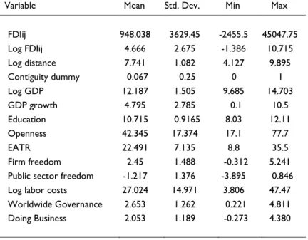
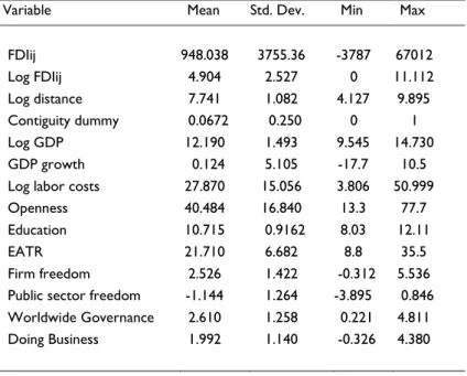
The Appendix presents a set of summary statistics for cross-section (see Table A.4) and panel data (see Table A.6).
Methodology
Empirical studies concerning FDI are usually based on some variation of the gravity model employed in empirical models of bilateral trade. Although in the trade literature the gravity model has good theoretical support, in the case of FDI the use of this model still needs development of solid theoretical foundations. When applied to bilateral FDI, this model states that the greater the
14 The min-max standardisation method rescaled to the 0-10 range implies to convert each original
variable to an index according to the formula 𝑆𝑐𝑜𝑟𝑒𝑘= 10 𝑓𝑎𝑐𝑡𝑜𝑟𝑘−𝑓𝑎𝑐𝑡𝑜𝑟𝑚𝑖𝑛
𝑓𝑎𝑐𝑡𝑜𝑟𝑚𝑎𝑥−𝑓𝑎𝑐𝑡𝑜𝑟𝑚𝑖𝑛 if higher factor
values imply better performances or 𝑆𝑐𝑜𝑟𝑒𝑘= 10 − 10𝑓𝑎𝑐𝑡𝑜𝑟𝑓𝑎𝑐𝑡𝑜𝑟𝑘−𝑓𝑎𝑐𝑡𝑜𝑟𝑚𝑖𝑛
𝑚𝑎𝑥−𝑓𝑎𝑐𝑡𝑜𝑟𝑚𝑖𝑛 if higher factor values
112
economic mass of the countries involved and the smaller the distance between them, the greater is the expected bilateral FDI. The usual procedure in trade literature is to add variables to the simplest gravity specification. In our paper we also use an augmented version of the gravity equation that includes economic, geographical and institutional variables affecting inward FDI.
Institutional variables considered in our model present a high degree of correlation between components, which leads to multi-collinearity problems in case of simultaneous inclusion of all variables that compose the three indicators previously introduced. Following Júlio et al. (2013), we solved this problem running, for each year, and for each one of the three institutional indicators used, a Principal Component Analysis (PCA), followed by a varimax rotation, in order to summarise data into a smaller set of indicators.
Using the standard eigenvalue-based criterion, with a cut-off 1, we identify two different components in the Index of Economic Freedom, explaining 67 percent of total variance. The rotated factor loadings matrix associates the first component score with indicators such as property rights, freedom from corruption, business freedom, investment freedom and financial freedom. The second component score is associated with indicators such as fiscal freedom and government spending (see Table A. 15 and Table A. 16 of the Appendix). Results are in line with Júlio et al. (2013), and for this reason we also decided to call the first component ‘firm freedom’, as it is associated with elements that influence the activity and profitability of companies, and the second component ‘public sector freedom’, as it measures the public sector effect on economic freedom. Applying the PCA to the six governance variables from the Worldwide Governance Indicators, we identify a component explaining 84 percent of total variance (see Table A. 17 and Table A. 18 of the Appendix). The component score - hereinafter Worldwide Governance - is interpreted as a broad measure of the quality of governance. Finally, the PCA identifies two components on the nine areas of Doing Business database, based on the standard eigenvalue-based criterion. Since factor loadings are difficult to associate to specific components and with a particular institutional feature, our option was to extract only one factor loading - hereinafter termed Doing Business – which is interpreted as a broad indicator of the ease of doing business. This component represents 46 percent of total variance, and is positively correlated with all nine areas of the Doing Business database (see Table A. 19 and Table A. 20 of the Appendix).
The score vectors resulting from the procedure described above are orthogonal to each other, diminishing the correlation among components of institutional indicators used. This procedure was accompanied by a Kaiser-Meyer-Olkin (KMO) test, which measures the sampling adequacy and confirmed the PCA as appropriate. The newly created institutional variables are then included in equations as regressors to capture the effect of institutions on FDI. New institutional variables were combined in order that different dimensions of institutions were covered without causing near multi-collinearity problems.
113 Cross-section
In the cross-section specification we explain average inward FDI for the 2008-2011 period using regressors dated 2007, with the exception of the mean years of schooling, which were collected for the year of 2010, due to data restrictions. The approach is intended to minimise potential endogeneity problems.
Denoting the source country by j and the host country by i, we initially estimate the following log-linear augmented gravity-type equation:
ln(FDIij) = cj + DISTANCEijβ1 + ECONiβ2 + INSTiβ3 + εij (4.1)
where FDIij is the FDI stock from country j to country i, DISTANCEij is a vector composed of the
distance between the capitals of countries i and j and the border dummy variable, ECONi is the
vector containing economic variables of the host country (GDP, GDP growth, the degree of openness, education, labour costs and EATR), and INSTi is a vector containing the institutional
variables of the host country. The vectors β1, β2 and β3 contain unknown coefficients to be estimated; and cj is a fixed effect that captures all idiosyncratic characteristics of the source country
affecting its volume of outward FDI, like GDP or institutional framework.15 Finally, ε
ij is an i.i.d.
error term assumed to be normally distributed. The variables FDIij, 𝐺𝐷𝑃𝑖, distance between
countries’ capitals and labour costs enter in (4.1) in logarithmic form.
The log specification is usually preferred in literature because it typically shows the best fit to the data, as suggested by Stein and Daude (2007a). However, this approach poses a problem when using the log of FDI as dependent variable, as the logarithm of zero is not defined. This problem has been dealt with in different ways. Some authors (Rose, 2000) simply drop all zero observations. This approach could lead to biased estimates, as those observations may contain important information. An alternative approach is to use a simple transformation and work with ln(1+ FDI)16 instead of ln(FDI), although Flowerdew and Aitkin (1982) demonstrate that adding small positive values makes estimates highly sensitive to the choice of the specific value added. Another way to deal with zero observations is to use a Tobit model (Stein and Daude, 2007a), considering that we have a censored-sample problem. This approach is based on the assumptions that stocks below a certain threshold are incorrectly recorded as zeros, because of rounding in FDI statistics, or that zeros are a consequence of fixed cost of investing abroad for investments below a certain threshold, despite the desired level of investment being positive.
15 This fixed effect enters in the equation as a vector of source country dummy variables.
114
We perform an OLS estimation of (4.1) using as depend variable ln(FDI), excluding zeros, and using ln(1+FDI) as alternative. Furthermore, we also estimate (4.1) using a Tobit model assuming a threshold of ln(1/4).17
The consistent estimation of the log-linearized model relies critically on the assumption that the εij
is not correlated with the regressors. Santos Silva & Tenreyro (2006) present strong evidence that this assumption may not hold, as the estimation of (4.1) by OLS or Tobit may lead to inconsistent estimates. The same authors thus recommend estimating such models in the multiplicative form and propose a Poisson pseudo-maximum-likelihood estimator, stressimg that, besides solving the inconsistency problem, a PPML estimator rightly deals with zero-FDI values.
The specification of the equation to be estimated is:
FDIij = exp[cj + DISTANCEijβ1 + ECONiβ2 + INSTiβ3]ϕij (4.2)
where ϕij = exp(εij).
Sometimes we found that the institutional indicators were highly correlated with some of the economic variables. Whenever this problem arose, we opted to not include the correlated variables together in the same regression. This resulted in alternative model specifications.
To check the adequacy of the estimated models, we performed the RESET test (Ramsey, 1969) and a Pregibon (1980) link test, both in their heteroskedasticity-robust versions. These tests try to identify whether there are omitted variables or misspecification of the functional form of the model. Despite some similarities, these two tests differ in the regressors used to test the misspecification. RESET is performed by fitting the original model augmented by the powers of the fitted values of the dependent variable (𝑌̂), while the link test is performed by fitting the original model augmented by the fitted values of the independent variables (𝐱𝛃̂). The aim is to detect if the new added variables help to explain the dependent variable. If so, there is evidence of misspecification. These two tests generally produce similar results for linear models, although, for non-linear models they can yield different outcomes. For that reason we decided to perform both tests.
Panel data
In the panel data specification we explain annual inward FDI stock using regressors collected for the previous year as a way to avoid simultaneity problems. Ideally, the dependent variable should be the tradable sector FDI average stock. However, due to the short time span of data available (four years), we opted to use annual stocks, instead of average stocks. Hence, FDI positions are not purged from the influence of price changes that can affect FDI’s valuation, which means that sectional and panel data results may not be fully comparable. All regressors used in the
115 section specification are also included in the panel regression. Additionally, we also included a fixed time-effect (µt)18, whose component is intended to capture all forms of time-varying heterogeneity
thataffectallcountry-pairssimilarly.The panel data version of the gravity log-linearised equation is:
ln(FDIijt) = cj + µt + DISTANCEijβ1 + ECONit−1β2 + INSTit−1β3 + εijt (4.3)
Westerlund & Wilhelmsson (2009) argue that the conventional approach of applying OLS to the log-linearized model with panel data is likely to cause bias and misleading inference even when the proportion of zeros is very small. They also point out that the PPML estimator adequately handles the zero-FDI observations and solves the heteroskedasticity problem (as referred to in Section 2) while dealing with the bias caused by country specific heterogeneity. In this sense, we will also estimate the following equation using a PPML estimator:
FDIijt = exp[cj + µt + DISTANCEijβ1 + ECONit−1β2 + INSTit−1β3]ϕijt (4.4)
Gravity models usually contain many time-invariant or nearly time-invariant regressors. In our model, variables such as distance, education and border dummies are time-invariant. Using the traditional fixed effects estimator, all these variables would be omitted from the regression, however, these variables are key to our analysis. Additionally, using the same set of variables in the panel and in cross-section specifications allows us to compare the results obtained. In this sense, we decided not to use the traditional fixed effect estimation method. Given that we control for source country fixed effects, only the host country remains with unobserved heterogeneity (and possibly some country-pair which, given the others, should be irrelevant). However, as there are many observed controls in the model specific to the host country, it is likely that host country unobserved heterogeneity will be not so important. Despite this, we are aware that both cross-section and panel estimations risk would be biased if these uncontrolled host heterogeneity is correlated with the regressors. However, we have no sound conjecture that makes us suspect the relevance of such a problem with this application, nor is it mentioned in the literature.
To perform the econometric estimation of equation (4.3) and (4.4) we used the pooled OLS and the pooled PPML. The random effects estimators are not used, as they are based on stronger assumptions, namely that observations are time-independent, which is hard to verify in practice. We assume that relevant unobserved heterogeneity is captured by the fixed time effect (µt) and by the source country fixed effect (cj).19 The estimated standard errors are heteroskedasticity robust
and allow for intragroup correlation and group heteroskedasticity, sweetening the requirement
18 The addition of a fixed time-effect can minimise the FDI’s valuation problem, but it does not eliminate it,
as price changes can be idiosyncratic.
19 We have also estimated the equations presented above including a host country fixed effect, however, the
116
that the observations are independent, which means that observations are independent across groups (clusters), but are not necessarily independent within groups.
To check the adequacy of the models, we performed a RESET test and a Pregibon link test, both heteroskedasticity-robust.
Results
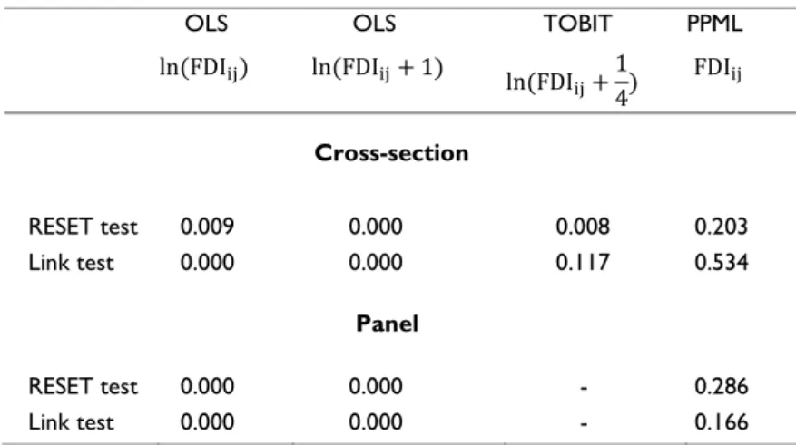
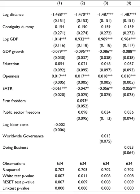
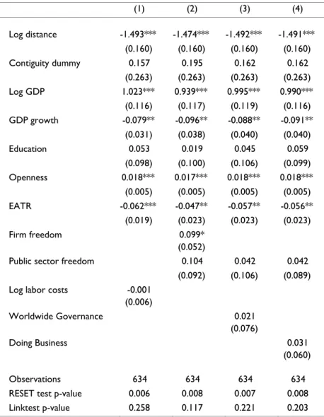
Table 1 reports the results of the two specification tests performed. The results of these tests and all other results presented in this section were obtained with Stata (StataCorp., 2011). Table 1 presents only the least favourable p-values obtained with each method20 (the highest when the null hypothesis is rejected and the lowest otherwise). In the OLS regressions, both tests reject the null hypothesis that the coefficient of the test regressor is 0. This means that the models estimated using the logarithmic form are misspecified. A similar result is found for the Tobit in the RESET test. In contrast, all the models estimated using the PPML regressions pass the RESET and Pregibon link test, that is to say, both tests provide no evidence of misspecification.
Below we focus on the analysis of the PPML results, as this method is able to deal with zero-FDI values in a suitable way, relies on weaker assumptions than other methods and, most of all, it is the only one that shows no evidence of misspecification simultaneously in both tests – see Table 1.
OLS OLS TOBIT PPML
ln(FDIij) ln(FDIij+ 1) ln(FDI
ij+14) FDIij
Cross-section
RESET test 0.009 0.000 0.008 0.203
Link test 0.000 0.000
Panel
0.117 0.534
RESET test 0.000 0.000 - 0.286
Link test 0.000 0.000 - 0.166
Least favourable p-values for each method - the highest when the null hypothesis is rejected and the lowest otherwise.
Table 1: Results of the specification tests (p-values)
20 We estimated four different equations with each estimator. These equations differ by including different
117 Nevertheless, whenever it is deemed appropriate, we compare PPML results with those obtained by OLS and Tobit. The OLS and Tobit outcomes, corresponding to the estimation of Equations 4.1 and 4.3, can be seen in Table A.8 to A.12 of the Appendix.21 Finally, we also compare our cross-section PPML results with those of Júlio et al. (2013), obtained for aggregated FDI with a very similar model. This last comparison should be analysed and interpreted with caution as, despite the models being quite similar, the time period and the samples used are different, and the results are not fully comparable.
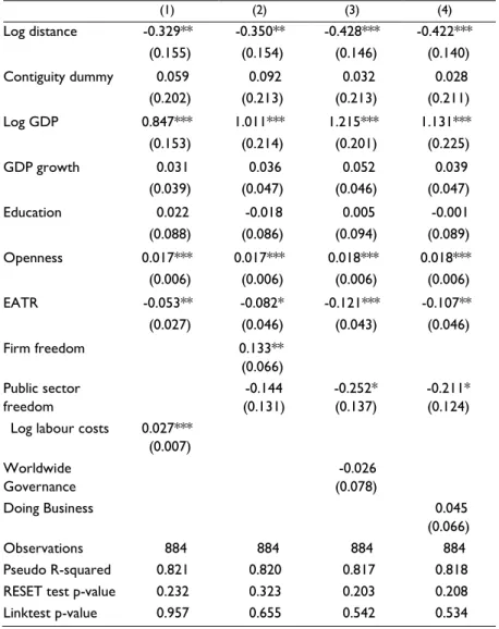
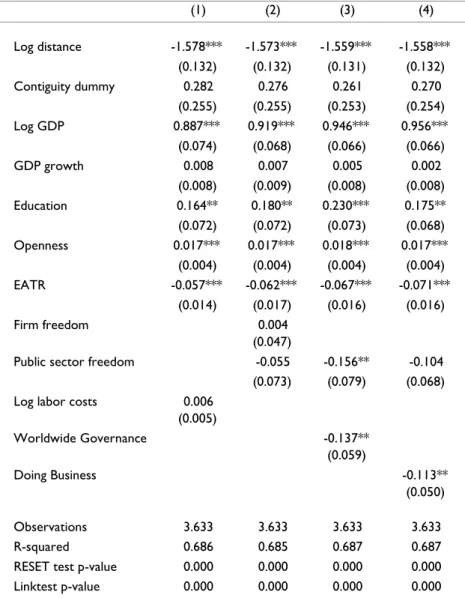
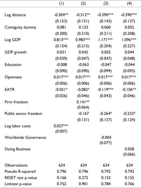
Table 2 below reports the outcomes from the cross-section PPML estimation (Equation 4.2) and Table 3 presents the results of the panel data PPML estimation (Equation 4.4). The first column of each table reports the results of the baseline regression, in which no institutional variable is included. We should interpret this column results with caution, as the regression may suffer from omitted variable bias. Columns (2) to (4) present different combinations of independent institutional variables. The combination of variables was made in order to achieve a good characterisation of the institutional framework and, simultaneously, avoid problems caused by near multi-collinearity of some institutional variables.22 This approach is also a way of assessing the robustness of the results obtained. Collinearity diagnostics tests were performed, after the estimation of the models, and none of the four specifications (combinations of variables) present a significant collinearity problem according to the VIF (variance inflation factor) measure.
Cross-section results
Table 2 reports the cross-section PPML estimates. These regressions leave out 128 pairs of countries with negative bilateral FDI (884 country pairs, out of 1,012, or 87% of the sample, and that they exhibit a non-negative average FDI position, as can be seen in Table A.3 of the Appendix). As a comparison, the OLS estimation technique, using the logarithm of FDI as dependent variable, leaves out 378 pairs of countries, which means that only 63% of the sample is used because of the zeros and negative bilateral FDI positions.
The PPML-estimated coefficients differ significantly from those obtained using OLS and Tobit (see Table A.8 to A.10 of the Appendix). On the other hand, they are very similar to the PPML coefficients estimated using only the positive-FDI subsample (see Table A.13 of the Appendix).
21 The OLS results presented in Table A.8 and A.11 were obtained using log of bilateral FDI as depend variable,
which means that all zero values are dropped. On what concerns to Table A.9 and Table A.12 results, the dependent variable considered is log of bilateral FDI+1, as a way to avoid the loss of zero observations. Although adding small values to the dependent variable is not the best solution to deal with the zeros problem, as mentioned in Section 4, it is important to measure and understand the impact on the estimates of the two different approaches.
22 Collinearity problems are mostly caused by high correlation between institutional variables, as can be seen
118
These results suggest that heteroskedasticity in the multiplicative error is the main cause for the difference between PPML results and those of OLS.
PPML estimates reveal that the role of geographical distance is much smaller than the one obtained using other methods: the estimated PPML elasticities oscillate between -0.33 and -0.43. These results mean that an increase of 1 percent in the number of kilometers between source and host countries is expected to reduce, on average, tradable sector FDI between 0.33 and 0.43 percent. OLS and Tobit estimates for these coefficients vary between -1.47 and -1.64. Júlio et al. (2013) using as depend variable aggregated FDI, estimated PPML elasticities that oscillate between -0.54 and -0.6323, which may lead us to conclude that distance seems to be an obstacle that is harder to overcome for aggregated FDI than for tradable sector FDI.
Results concerning contiguity are similar for different estimation methods and combination of variables, and they reveal that sharing a common border does not affect inward FDI into the tradable sector. This outcome differs significantly from the results obtained by Júlio et al. (2013), and from the results that have usually been obtained in the literature for aggregated FDI. Júlio et al. (2013) found that the FDI of a country in its neighbour is approximately between 73 and 88 percent higher than the FDI in a similar country that does not share a common border. Border and distance results show that physical distance does not represent a major obstacle to the attraction of FDI into the tradable sector.
The level of GDP is always statistically significant, which supports the economic mass hypothesis. PPML estimated GDP elasticities are around 1 (the null hypothesis of a unit elasticity is never rejected at the usual significance levels in any of the estimated equations). These results are in line with the GDP elasticities we obtained with other estimators,and with the empirical results obtained in the literature for aggregated FDI.
The effect of economic growth and education does not seem to be significant when we use the PPML estimator. However, for all other estimation methods used, economic growth is statistically significant and plays a negative role on FDI. One possible explanation for this statistical insignificance is that local market growth is not crucial to FDI because, usually, tradable sector production is not targeted only to the national market, but also to the world market. The statistical insignificance of education may result from two opposite effects that cancel each other out. On the one hand, more education implies higher productivity, yet, on the other, it is also associated with higher wage costs. As we have controlled for the labour costs’ effect, the result suggests that the productivity effect captured by the education variable does not seem to be relevant to the attraction of tradable sector FDI. Júlio et al.’s (2013) PPML estimates presented some statistical evidence of a negative effect of education, and of a positive effect of economic growth on FDI.
23 Estimated elasticities in literature oscillate between -1.9 (Stein and Daude, 2007a) and -0.49
119
(1) (2) (3) (4)
Log distance -0.329** -0.350** -0.428*** -0.422***
(0.155) (0.154) (0.146) (0.140)
Contiguity dummy 0.059 0.092 0.032 0.028
(0.202) (0.213) (0.213) (0.211)
Log GDP 0.847*** 1.011*** 1.215*** 1.131***
(0.153) (0.214) (0.201) (0.225)
GDP growth 0.031 0.036 0.052 0.039
(0.039) (0.047) (0.046) (0.047)
Education 0.022 -0.018 0.005 -0.001
(0.088) (0.086) (0.094) (0.089)
Openness 0.017*** 0.017*** 0.018*** 0.018***
(0.006) (0.006) (0.006) (0.006)
EATR -0.053** -0.082* -0.121*** -0.107**
(0.027) (0.046) (0.043) (0.046)
Firm freedom 0.133**
(0.066) Public sector
freedom
-0.144 (0.131)
-0.252* (0.137)
-0.211* (0.124)
Log labour costs 0.027***
(0.007) Worldwide
Governance
-0.026 (0.078)
Doing Business 0.045
(0.066)
Observations 884 884 884 884
Pseudo R-squared 0.821 0.820 0.817 0.818
RESET test p-value 0.232 0.323 0.203 0.208
Linktest p-value 0.957 0.655 0.542 0.534
Robust standard errors in parentheses. *** p<0.01, ** p<0.05, * p<0.1.
Source country dummies were included, but not reported.
Table 2: Cross-Section PPML estimates
120
(2013) PPML estimates for EATR are not always statistically significant, meaning that tax competitiveness should be taken into account for countries seeking to attract FDI into tradable sectors. Effective average tax rate reflects tax incentives, such as investment tax credits granted to companies when investments are made, and validates this kind of economic policies as being a way to attract foreign direct investment into the tradable sector.24
Labour costs is statistically significant only in the PPML estimation and impacts FDI positively. The results in Júlio et al. (2013) for this variable suggest a negative effect for aggregated FDI. This opposite result suggest that productivity gains for tradable sector FDI, which are positively associated with labour costs, overcome the negative effect of higher wages, while for aggregated FDI the opposite holds.
Institutional variables Firm freedom, Worldwide Governance and Doing Business are highly correlated and were not included simultaneously in the regressions. Results in Table 2 suggest that Firm Freedom and Public Sector Freedom were the only institutional variables to play a role in tradable sector FDI. These two variables seem to impact FDI, positively and negatively, respectively. Worldwide Governance and Doing Business are non-significant. Júlio et al.’s (2013) PPML estimates for Firm fFreedom, Public Sector Freedom and Doing Business were consistent with our estimates in terms of signal. The main difference is that they find a non-significant effect of Public Sector Freedom on aggregated FDI and their estimates for the Firm Freedom coefficient (varying between 0.53 and 0.76) are substantially larger than our estimate (0.13).
Firm Freedom is associated with indicators such as protection of property rights, freedom from corruption, investment and business freedom, and, in this sense, societies that guarantee these set of rights and freedoms to foreign investors will surely attract more FDI.
Public sector freedom is associated with indicators such as fiscal freedom and government spending. Theoretically, it is not clear whether higher public expenditure should attract or repeal FDI. On the one hand, a strong state presence in the economy takes space from private enterprises. On the other hand, higher public expenditures may be associated with good infrastructures, stable socioeconomic conditions, and strong public incentives for FDI.
Our results support the idea that state intervention in the economy could have a positive effect for the attraction of FDI into the tradable sector, although the evidence is weak (the coefficient is only statistically significant at the 10 percent level).
24 Our results are in line with those of Cassou (1997), who found that host country corporate tax rates have
121 Panel data results
In this sub-section, we extend our analysis to assess the tradable sector FDI determinants over time. Besides representing an additional robustness check to cross-section results, the panel data model allows us to have more observations and to control for the time-varying heterogeneity by means of a fixed time effect.
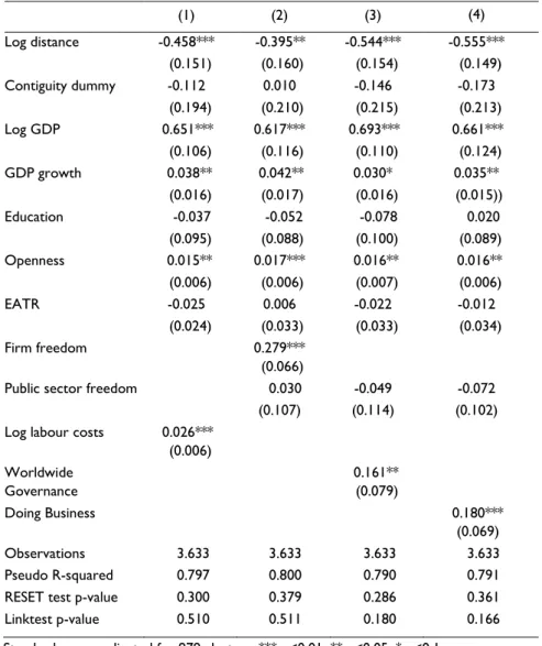
Table 3 shows the panel pooled PPML estimates with clusters-robust standard errors. These regressions leave out 415 observations with negative bilateral FDI (3,633 country pair observations, out of 4,048, or that 90% of the sample exhibit a non-negative FDI position, as can be seen in Table A.3 of the Appendix). Once again, estimating the model in logarithmic form through OLS leaves out 1,707 pairs of countries due to non-positive FDI positions, which is the equivalent to 42 percent of the sample. As the pairs of countries do not leave the panel randomly, the loss of observations is more severe in small countries or countries where the manufacturing sector has a smaller relative size. Hence, the panel become highly unbalanced. This means that the impact of zero observations in our sample is more severe in panel data and to simply drop this data will likely lead to a serious estimation bias.
Pooled PPML coefficients differ significantly from those obtained using pooled OLS the same way that cross-section PPML estimates diverge from cross-section OLS. Furthermore, PPML estimated coefficients are very similar when using the whole sample and the positive-FDI subsample (see Table A.14 of the Appendix). These results suggest that heteroskedasticity in the multiplicative error is the main cause of the difference between PPML and OLS results, as was observed for the cross-section data.
The role of geographical distance as a FDI deterrent is a bit higher for pooled PPML than for cross-section PPML - an increase of 1% in the number of kilometers between source and host countries is expected to reduce tradable sector FDI between 0.40% and 0.56%. The contiguity dummy estimated coefficients show that sharing a common border does not affect inward FDI. These results support the hypothesis that distance is no obstacle to transpose tradable sector FDI.
Results obtained for GDP level are somewhat different from those of pooled OLS and of cross-section models. In particular, estimated elasticities now oscillate between 0.62 and 0.69, while pooled OLS estimates vary between 0.89 and 0.95, and cross-section estimated GDP elasticities are close to 1. These results still support the economic mass hypothesis, but rule out the hypothesis of a unit elasticity of level GDP (the null hypothesis of a unit elasticity is unequivocally rejected at any usual significance level).
122
effect on FDI, while in a cross-section framework it is non-significant. Education and EATR do not seem to affect FDI based on the results of Table 3. EATR statistical insignificance contradicts the cross-section PPML results, and puts into doubt the idea of attracting FDI into tradable sector through policies that promote countries’ tax competitiveness. The effect of labour costs on FDI is statistically significant and is in line with the cross-section results in terms of economic significance, which consolidates the idea that with tradable sector FDI, productivity gains, which are positively associated with labour costs, overcome the negative effect of higher wages.
(1) (2) (3) (4)
Log distance -0.458*** -0.395** -0.544*** -0.555***
(0.151) (0.160) (0.154) (0.149)
Contiguity dummy -0.112 0.010 -0.146 -0.173
(0.194) (0.210) (0.215) (0.213)
Log GDP 0.651*** 0.617*** 0.693*** 0.661***
(0.106) (0.116) (0.110) (0.124)
GDP growth 0.038** 0.042** 0.030* 0.035**
(0.016) (0.017) (0.016) (0.015))
Education -0.037 -0.052 -0.078 0.020
(0.095) (0.088) (0.100) (0.089)
Openness 0.015** 0.017*** 0.016** 0.016**
(0.006) (0.006) (0.007) (0.006)
EATR -0.025 0.006 -0.022 -0.012
(0.024) (0.033) (0.033) (0.034)
Firm freedom 0.279***
(0.066)
Public sector freedom 0.030 -0.049 -0.072
(0.107) (0.114) (0.102)
Log labour costs 0.026***
(0.006) Worldwide
Governance
0.161** (0.079)
Doing Business 0.180***
(0.069)
Observations 3.633 3.633 3.633 3.633
Pseudo R-squared 0.797 0.800 0.790 0.791
RESET test p-value 0.300 0.379 0.286 0.361
Linktest p-value 0.510 0.511 0.180 0.166
Standard errors adjusted for 979 clusters. *** p<0.01, ** p<0.05, * p<0.1
Source country and time dummies were included, but not reported
123 Table 3 results also stress that the institutional variable Firm Freedom, as in cross-section framework, plays an important role for the attraction of tradable sector FDI. The estimated coefficient is 0.28 in pooled PPML, while in cross-section it is only 0.13, which are both statistically significant at the 5 percent level. Public Sector Freedom is not statistically significant. This result contradicts cross-section outcomes for this variable, in the sense that it does not support the idea that state intervention in the economy has a positive effect on FDI.
Worldwide Governance and Doing Business seems to impact FDI positively in pooled PPML regressions, while in cross-section, they are not statistically significant. Thus, according to these results, countries presenting a better governance, more efficiency and less bureaucracy are expected to attract more FDI. Panel data results do not always coincide with those of cross-section. On the one hand, the difference between panel and cross-section results can be explained by the different nature of the dependent variable. In cross-section, the dependent variable is a 4-years FDI average stock, while in the panel specification, it is the annual inward FDI stock. Thus, panel data FDI positions are not purged from the influence of price changes that can affect FDI’s valuation. On the other hand, panel data allow us to use more observations, taking advantage of the increased sample variability, and also enables us to control for the unobserved heterogeneity by using a fixed time effect.
Conclusion
Most of the literature on FDI has focused on aggregated FDI determinants. A usual conclusion from these studies is that the physical distance between countries is a first order determinant of the aggregated FDI. In this paper we focused on the tradable sector FDI determinants, showing that distance between source and host countries does not represent an obstacle that is too hard to transpose for tradable sector FDI, as it seems to represent aggregated FDI. In fact, to share a border does not seem to have an impact on the attraction of FDI to the tradable sector, while it seems to play an important role in the attraction of aggregated FDI. On the other hand, our results stressed that the degree of economic openness of a country is much more important for the attraction of tradable sector FDI than aggregated FDI. Finally, this paper also presents evidence that productivity gains, which are positively associated with labour costs, overcome the negative effect of higher wages for tradable sector FDI, while for aggregated FDI the opposite usually holds.
124
References
Ali, F., (2010). “Essays on foreign direct investment, institutions, and economic growth.” PhD thesis, University of Glasgow.
Altomonte, C. and Guagliano, C., (2003), “Comparative study of FDI in Central and Eastern Europe and the Mediterranean,” Economic Systems, 27 223-246.
Bajo-Rubio, O. and Sosvilla-Rivero, S., (1994), “An econometric analysis of foreign direct investment in Spain, 1964-89”, Southern Economic Journal, 61 104-120.
Barrell, R. and Pain, N., (1996). “An econometric analysis of U.S. foreign direct investment,” The Review of Economics and Statistics, 78 200-207.
Barro, R. and Jong-Wha L., (2010), "A New Data Set of Educational Attainment in the World, 1950-2010." Journal of Development Economics, 104 184-198.
Bénassy-Quéré, A., Coupet M. and Mayer, T., (2007). “Institutional determinants of foreign direct investment,” The World Economy, 30 764-782.
Billington, N., (1999). “The location of foreign direct investment: an empirical analysis,” Applied Economics, 31 65-76.
Biswas, R., (2002). “Determinants of foreign direct investment,” Review of Development Economics,
6 492-504.
Botero, J., Djakov, S. La Porta, R., Lopez-de Silanes F. and Shleiffer, A.,(2004). “The regulation of labor.” Quarterly Journal of Economics, 119 1339-1382.
Borensztein, E., De Gregorio J. and Lee, J. (1998). “How does foreign direct investment affect economic growth?” Journal of International Economics, 45 115-135.
Buch, C., Kleinert, J., Lipponer A. and Toubal, F., (2005). “Determinants and effects of foreign direct investment: evidence from German firm-level data,” Economic Policy, 20 52-110.
Cassou, S., (1997). “The link between tax rates and foreign direct investment,” Applied Economics,
29 1295-1301.
Cheng, I.-H., and Wall, H. J., (2005). “Controlling heterogeneity in gravity models of trade and integration,” Review of the Federal Reserve Bank of St. Louis, 87 49-63.
Cheng, I.-H., and Tsai, Y.-Y., (2008). “Estimating the staged effects of regional economic integration on trade volumes,” Applied Economics, 40 383-393.
125 Devereux, M. and Griffith, R., (2003). “Evaluating Tax Policy for Location Decisions," International Tax and Public Finance, 10 107-126.
Djankov, S., Porta, R. L., de Silanes, F. L., and Shleifer, A., (2008). “The law and economics of self -dealing,” Journal of Financial Economics, 430-465.
Flowerdew, R. and Aitkin, M., (1982). “A method of fitting the gravity model based on poisson distribution,” Journal of Regional Science, 22(2) 191-202.
Hartman, D., (1984). “Tax policy and foreign direct investment in the United States,” National Tax Journal, 37 475-487.
Hartman,D.,(1985).“Taxpolicy and foreign direct investment,”Journal of PublicEconomics,107-121.
Higgins, M., and Klitgaard, T., (2014). “The Balance of Payments Crisis in the Euro Area Periphery,”
Current Issues in Economics and Finance, 20(2)
Hines, J., (1996). “Altered states: taxes and location of foreign direct investment in America”,
American Economic Review, 86 1976-1094.
Júlio, P., Pinheiro Alves, R., and Tavares, J., (2013). "Foreign direct investment and institutional reform: evidence and an application to Portugal," Portuguese Economic Journal, 12 215-250.
Kinoshita, J., “Sectoral Composition of Foreign Direct Investment and External Vulnerability in Eastern Europe,” IMF Working Paper 11/123, International Monetary Fund.
Kaufmann, D., A. Kraay, and P. Zoido-Labatón, (1999). “Governance matters,” World Bank Policy Research Working Paper, 2196 Washington, DC.
Knack, S. and Keefer, P., (1995). “Institutions and economic performance: cross-country tests using alternative institutional measures,” Economics & Politics, 7 207-227.
Kravis, I. and Lipsey, R., (1982). “The location of overseas production and production for exports by U.S. multinational firms,” Journal of International Economics, 12 201-223.
Larraín, B. and Tavares, J., (2004). “Does Foreign Direct Investment Decrease Corruption?" Latin American Journal of Economics, 41 217-230.
Lee, J.-Y. and Mansfield, E., (1996). “Intellectual property protection and U.S. foreign direct investment,” The Review of Economics and Statistics, 78, 199-215.
Proença, I., Sperlich, S., Savasci, D., (2015). “Semi-mixed effects gravity models for bilateral trade,”
Empirical Economics, 48 361-387.