www.IJoFCS.org
FORENSIC COMPUTER SCIENCE
Noise-Robust Speaker Recognition using Reduced
Multiconditional Gaussian Mixture Models
Frederico Q. D’Almeida, Francisco Assis Nascimento, Pedro de A.
Berger, and Lúcio M. da Silva
Abstract – Multiconditional Modeling is widely used to create noise-robust speaker recognition systems. However, the approach is computationally intensive. An alternative is to optimize the training condition set in order to achieve maximum noise robustness while using the smallest possible number of noise conditions during training. This paper establishes the optimal conditions for a noise-robust training model by considering audio material at different sampling rates and with different coding methods. Our results demonstrate that using approximately four training noise conditions is sufficient to guarantee robust models in the 60 dB to 10 dB Signal-to-Noise Ratio (SNR) range.
Keywords – Automatic speaker recognition, Gaussian mixture models, Multiconditional models, noise robustness, computing power.
1. Introduction
Modern Automatic Speaker Recognition (ASR) systems, based on Gaussian Mixture Models (GMMs) and using Mel Frequency Cepstral Coefficient (MFCC) parameters, have proven to be quite successful at identifying the author of a voice extract. Nevertheless, a limiting factor for the performance of such systems is the quality of the source material available for comparison. In order to make ASR systems robust to noise, a common strategy is to use Multiconditional Model Training (Lippmann et al., 1987; Deng et al., 2000; Ming et al., 2007a). This approach models the speaker’s voice using a number of low complexity models of the same speaker, each one trained at a particular Signal-to-Noise Ratio (SNR). Recently, Ming et al. (2007b) employed a variation of this
technique where a single complex model with a large number of Gaussian components was trained simultaneously with different SNR samples. This approach was a replacement for training with a group of simple models. Despite the consistent improvement in the model’s noise tolerance, both approaches produced a remarkable increase in model complexity and, consequently, in the computational cost of the overall task.
the robustness of the system. However, for most speaker recognition applications, response time and processing power are limiting factors that can preclude excessive model complexity.
The goal of this paper is to present a comprehensive study on the performance of ASR systems under different noise conditions, and to explore the optimal audio database for testing signals at different sampling rates and with different coding methods. In particular, we explore the precise system performance degradation that results from testing models under mismatched noise conditions. We also show that it is possible to effectively determinate the relevant SNR for the multiconditional model training that simultaneously guarantees noise robustness and keeps the model’s complexity low. In this sense, our work proposes a low-complexity model that has little effect on performance degradation (in comparison to the complete model) while also maintaining a low overall computational cost.
2. Multicondition Model
Speaker recognition systems based on GMM using MCFF parameters are a widely employed, successful technique for recognizing voice excerpts in large speaker databases when the audio has not been corrupted by noise (Campbell, 1997). Noisy speaker recognition systems, however, are still under development. The most common technique when dealing with noisy speaker recognition systems is multiconditional model training. This technique builds noise-robust speaker models by incorporating noisy audio to the model training.
In order to set up a multiconditional model, several training audio sets at different noise levels must be available. Here we represent these training data sets as Φn, where the index n refers to the noise level. Often, these training sets are built up from a single noiseless training database,Φ0 by adding progressive amounts of simulated white noise.
In traditional multiconditional model training, each training data set Φn is used to train one
specific speaker model. The set of models for each speaker is then combined to form the multiconditional model. This is mathematically represented by
(
)
(
) (
)
0|
| ,
|
N n n np X S
p X S
P
S
=
=
∑
Φ
Φ
, (1)where X is a feature vector extracted from the test data, S represents the speaker,
p X S
(
| ,
Φ
n)
is the likelihood function of vector X for the speaker S trained on set Φn, and
P
(
Φ
n|
S
)
is the prior probability for the occurrence of noise condition Φn for speaker S. Obviously, the prior probabilities are restricted to(
)
0|
1
N n nP
S
=Φ
=
∑
. (2)If using GMM speaker models, each likelihood function
p X S
(
| ,
Φ
n)
has the form(
)
, ,( )
1
| ,
M
n n i n i
i
p X S
p b
X
=
Φ =
∑
, (3)where the pn,i are the mixture coefficients
and bn,i are the GMM components. The mixture
coefficients are restricted to
, 1
1
M n i ip
==
∑
, (4)since they are the prior probabilities of each Gaussian component in the GMM model. The GMM components bn,i are Gaussian distributions of the form
( )
( )
(
)
(
)
1
, , ,
, / 2 1/ 2
, 1 exp 2 2 T
i n i n i n
i n D
i n
x x
b x µ µ
π
−
− Σ −
= −
Σ
, (5)
where D is the dimension of the model.
method of treating the multiconditional training than the traditional scheme. As one can easily verify by inserting eq. into eq. , the multiconditional model can be re-written as
(
)
, ,( ) (
)
0 1
|
|
N M
n i n i n
n i
p X S
p b
X
P
S
= =
=
Φ
∑ ∑
. (6)After making a simple re-indexing from the dual reference n and i to the single reference k, we have
(
)
' '( )
( 1) ' '( )
, ,
0 1 0
|
N M
N M
n i n i k k
n i k
p X S p b X p b X
+
= = =
=
∑∑
=∑
, (7)where
(
)
(
)
' . , ' . ,|
|
n i n i n
n i n i n
p
p P
S
b
b P
S
=
Φ
=
Φ
. (8)Treating the multiconditional model as a unique large GMM model has the advantage of having only one constraint, namely
( 1) ' 0
1
N M k kp
+ ==
∑
, (9)while the traditional multiconditional model has N+1 constrains: one as indicated by eq. , and
N constraints from the multiple instances of eq. .
3. Model Reduction
Using any of the multiconditional model formulations inevitably causes a considerable increase in model complexity and the required computational power. The complexity of models grows linearly with N, the number of conditions used in the multiconditional training. Although this linear growth may not appear to be a severe problem for speaker recognition tasks, one must consider that the whole speaker set must be tested in order to find the author of a voice excerpt. Using multiconditional modeling means that the complexity of the entire speaker universe will grow by a factor of N, transforming a very large problem into an even larger one.
The most straightforward way of reducing the demanded computer effort in multiconditional
speaker recognition tasks is by minimizing the number of conditions used during model training. This reduction, however, must be strictly controlled in order to maintain the noise-robustness of the method. Building a multiconditional model that requires a minimum number of training conditions but is still robust to varying noise conditions requires an analysis of the exact effect that each training condition has on the overall system performance.
With this aim in mind, we have carried out a set of noise mismatch tests. Our mismatched testing procedure consists of submitting a system of uniconditional models, trained with unique noise conditions Φm, to speaker recognition tasks with questioned voice excerpts of different noise characteristics Ψn, where n = 1,…,N. Here,
Ψ represents the testing audio data set, which is different from the training data set Φ, and Ψn represents the audio data set Ψ at noise level
n. Although Φ and Ψ are different audio sets, the noise level in Φm is the same used in Ψn for every m = n. By doing this, the noise range that each individual uniconditional model represents can be determined. Thus, one can establish the optimal noise conditions set to build up the multiconditional model.
The actual mismatched testing was carried out by training uniconditional systems at 60 dB, 50 dB, 40 dB, 30 dB, 26 dB, 20 dB, 16 dB and 10 dB SNR audio sets (Φ0,…,Φ7), and testing each one at 60 dB, 50 dB, 40 dB, 30 dB, 26 dB, 20 dB, 16 dB and 10 dB SNR audio sets (Ψ0,…,Ψ7). The 60 dB SNR corresponds to the “noiseless” audio, as this is the average estimated SNR level of the original audio database. Additional mismatched testing was performed using different audio quantization schemes for the training and test.
4. Audio Database Description
speakers. Each recording was then fragmented in 21 files for a total of 630 audio extracts. The first and last cut points in these files were the same for all speakers in relation to the text content of speech. Thus, we generated 21 files for each speaker, with one used for model training (Φ0) and the other 20 used for testing (Ψ0). The duration of each voice extract was approximately 30 s.
All of the recordings were performed in acoustically prepared environments, using professional audio caption microphones and plates. The files were captured at a sample rate of 16 kHz, 16-bit quantization in monaural mode. From this initial audio database, three subsampled 8 kHz database versions were built for use in the simulations: one with 16-bits per sample, one with 8-bit µ-law coding, and one with 8-bit linear coding. A second database version resampled at 11 kHz and 16-bits was also used.
4.1 Pre-processing
All audio files were pre-processed before testing. First, each file was normalized such that the peak amplitude corresponded to 100% of the maximum quantization value. Each file’s silent extracts were then excluded. This was performed using an automatic silence detector based on the measure of the signal energy in 20 ms windows, with an overlap of 15 ms (5 ms advances) and a manually defined silence threshold. The silence threshold definition was performed by successively adjusting and retesting for verification.
4.2 Noise Addition
The noisy audio samples were generated from the “noiseless” audio database (Φ0, Ψ0) by adding a precise amount of Additive White Gaussian Noise (AWGN). The procedure was as follows. First, we calculated the average signal energy (Es) in the pre-processed audio extracts, given by
[ ]
2
s s
m
E
=
∑
y
m
, (10)where ys is the noiseless audio waveform and
m is the time index of the sample audio extracts.
A noise vector (yn) was then generated with the same dimension as the audio vector signal (ys) and containing zero mean Gaussian distributed samples. The energy (En) of this noise vector was also calculated, given by
[ ]
2
n n
m
E
=
∑
y
m
. (11)The noise vector amplitudes were then adjusted in order to get the desirable SNR, or
10
'
. 10
.
SNR s
n n
n
E
y
y
E
−=
. (12)Finally, the noise vector with adjusted amplitudes was added to the signal vector, resulting in the noisy audio vector (y), or
'
s n
y
= +
y
y
. (13)The SNRs used in the simulations were 60 dB, 50 dB, 40 dB, 30 dB, 26 dB, 20 dB, 16 dB and 10 dB, both for the training data sets (Φn) and the testing data sets (Ψn). As mentioned earlier, the 60 dB SNR audio is equivalent to “noiseless” audio since this is the average estimated SNR level of the original audio database. This SNR level was calculated based on the average signal energy of the speech and silent extracts of the entire audio database before preprocessing. In other words, the 60 dB SNR level has no noise added.
The noise addition procedure was performed on the 16 kHz / 16-bit original database using 32-bit arithmetic. The noisy databases were obtained by resampling and recoding the high coding audio set. This was done in order to avoid quantization error accumulation which would occur if the noise addition had been performed over the 8-bit audio.
of the noise signal (y’n) added to the signal is higher than it would be if we considered the original unedited audio file. Based on our tests, we concluded that the SNR values which were presented in this paper are roughly 10% higher than those obtained if the noise addition process was performed on the original audio extracts.
Note that we chose this particular methodology for measuring SNRs for a couple of reasons. First, since the locution rhythms and time pauses between words and phrases vary for distinct individuals, the measured SNR is sensitive to these particular individual characteristics. Therefore, it is possible to achieve distinct SNR values even if the signal and noise energy are kept fixed. Second, the identification of the extracts with voice and silent intervals is much simpler in noiseless audio (where we can use a simple energy detector) than in noisy audio.
Despite the fact that the noise addition was performed in a simulated computer environment, real ASR system tests assure that this procedure closely reproduces the real-world acoustic addition of noise (Ming et al., 2007b).
5. Recognition System
The recognition system used for performance evaluation is based on Gaussian Mixture Models (GMMs). This kind of speaker modeling is currently the widely employed and has yielded satisfactory results in ASR systems, especially for noisy situations (Graciarena et al., 2007; Reynolds et al., 1992; Rose et al., 1991).
As shown in eq. , GMMs are a combination of individual Gaussian models which are intended to represent the different vocal productions of a single person (Reynolds et al., 1992b). Each Gaussian of the composite GMM first models one specific sound class. In this way, the complete group of Gaussians is capable of modeling a large number of sound classes to an acceptable level of precision, and could therefore recognize the speaker independently of the spoken content.
For each simulation performed here, we used a 16 component GMM following the approach of Reynolds et al. (1995). Increasing the model complexity further does not significantly improve system performance. Also, for an additional simplification, the model covariance matrix was restricted to be diagonal. Such a restriction does not significantly impact the system results (Reynolds et al., 2000).
The GMMs were trained using Mel Frequency Cepstral Coefficients (MFCCs). This approach has proven to be a superior chose of parameters for speaker representation when compared to other parameterizations (D’Almeida et al., 2006; Jankowski et al., 1995). Additionally, this particular type of parameter is widely used in other ASR studies, which facilitates comparisons with the wider literature.
The MFCC parameters were calculated for each 20 ms window of audio, without window overlapping, through filter banks applied directly to the signal frequency spectrum as calculated in this same window. From each window, 12 parameters were extracted.1 After computing the MFCC parameters,
the cepstral mean subtraction procedure was applied as described in Reynolds et al. (1995), both for the training and testing phases. Spectral mean subtraction techniques are a well known tool to improve ASR systems performance (Schwartz et al., 1993; Jankowski et al., 1995; Vaseghi et al., 1997), which aim to minimize constant or slowly varying spectrum background noise.
6. Results
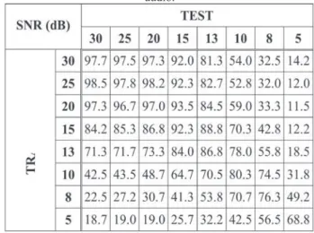
The system performance evaluation was computed using the correct speaker recognition ratio. For each situation (sampling frequency, training SNR and test SNR), 600 speaker recognition tasks were performed, one for each audio test sample (30 speakers multiplied by 20 test audio samples per speaker). The results of
1 The same number of 12 MFCC parameters was used for 16 kHz,
the complete mismatched testing procedure are organized into two-dimensional matrixes. Rows indicate how a system trained with a particular SNR performs for different noise test conditions, and columns indicate how a specific test SNR is handled by different training conditions. These results are displayed in tables 1 through 7, containing the correct recognition rates for each tested configuration. Each table refers to a specific audio coding and sampling frequency.
The mismatched testing was performed using different audio quantization schemes for model training and testing. The results of training the models with 16-bit audio and testing with 8-bit
µ-law audio are summarized in table 6. The results of training the models with 16-bit audio and testing with 8-bit linear audio are summarized in table 7.
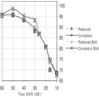
Our results show that it is possible to build noise-robust multiconditional models using a reduced set of conditions. For example, in the 16 kHz / 16-bit test audio, training conditions of 60 dB, 30 dB, 20 dB and 10 dB are enough to build a decent model that performs close to the full model. Fig. 1 shows a comparison of the best results for each noise condition considering all training conditions used (full set) and the reduced set. With the exception of the 30 dB noise condition, no significant performance differences were found between the reduced training set case and the full training set.
70 75 80 85 90 95 100
10 20 30 40 50 60
T e s t S N R ( d B )
Reduc ed Co mplet e
Fig. 1. Comparison of the best correct recognition rate results for each noise condition considering complete and reduced training sets. Testing and training model audio were sampled at 16 kHz and coded with 16-bits.
65 70 75 80 85 90 95 100
10 20 30 40 50 60
T e s t S N R ( d B )
Reduc ed Co mplet e
Fig. 2. Comparison of best correct recognition rate results for each noise condition considering complete and reduced training sets. Testing and
training model audio were sampled at 11 kHz and coded with 16-bits.
For the 11 kHz / 16-bit and 8 kHz / 16-bit test audio, the differences between the full training condition set and the reduced set is even less noteworthy, as seen in fig. 2 and fig. 3. In these simulations, the reduced set used was the same as in the 16 kHz case (60 dB, 30 dB, 20 dB and 10 dB). For the 8 kHz / 8-bit µ-law test audio, two sets of simulations were performed. We trained the models with the same audio codification scheme, and with using 8 kHz / 16-bit audio. Both situations are represented in fig. 4, where we find that although the test audios were coded at 8-bit
µ-law, the models trained with 16-bit audio had superior performance, especially for the low noise cases. For the reduced training condition models and for models trained with 8-bit µ-law audio, the optimal reduced condition training set is 50 dB, 26 dB, 20 dB and 10 dB. For models trained with 16-bit audio, the best reduced condition training set is 50 dB, 30 dB, 20 dB and 10 dB. With these reduced training conditions set, one can verify that the reduced model trained with 16-bit audio maintained good performance at the 16 dB noise level, while the reduced model trained with 8-bit
µ-law audio had a noticeable performance loss.
with 16-bit audio were less expressive. Again, models trained with 16-bit audio showed better performance. The optimal reduced conditions training sets for this case are 60 dB, 30 dB, 20 dB and 10 dB for models trained with 8-bit audio, and 50 dB, 30 dB, 20 dB and 10 dB for models trained with 16-bit audio.
65 70 75 80 85 90 95 100
10 20 30 40 50 60
T e st S N R ( d B )
Reduc ed Co mplet e
Fig. 3. Comparison of best correct recognition rate results for each noise condition considering complete and reduced training sets. Testing and
training model audio were sampled at 8 kHz and coded with 16-bits.
65
70
75
80
85
90
95
100
10
20
30
40
50
60
Test S N R ( dB )
Reduc ed
Complet e
Reduc ed, 16 bit
Complet e, 16 bit
Fig. 4. Comparison of best correct recognition rate results for each noise condition considering complete and reduced training sets. The testing
audio was sampled at 8 kHz and coded with 8-bit μ-law. This figure
shows the results for two sets of simulations: training the models with the same audio coding scheme as for the testing audio, and training with
audio sampled at 8 kHz and coded with 16-bits.
65 70 75 80 85 90 95 100
10 20 30 40 50 60
T e st S N R ( d b )
Reduc ed Co mplet e Reduc ed, 16 bit Co mplet e, 16 bit
Fig. 5. Comparison of best correct recognition rate results for each noise condition, considering complete and reduced training sets. The testing
audio was sampled at 8 kHz and coded with 8-bits. This figure shows
the results for two sets of simulations: training the models with the same audio coding scheme as for the testing audio, and training the audio
sampled at 8 kHz and coded with 16-bits.
7. Discussion
Reduced Multiconditional Models have proven to be a good technique to build noise-robust speaker recognition systems with minimal model complexity. By correctly choosing the training conditions set, it is possible to build speaker recognition systems that are robust up to 10 dB SNR using only four training conditions.
8. Conclusions
In this work, the performance degradation of ASR systems was analyzed as a function of test audio SNR mismatches with respect to the training audio SNR. The aim of this paper was to identify which audio SNR were relevant for model training in order to guarantee noise robustness and, at the same time, keep model complexity to a minimum. Out results indicate that, for the tested sampling frequencies and audio coding methods, a training model with only four selected noise conditions is sufficient to provide a level of noise robustness very close to that achieved by the full eight condition model. This leads to a 50% model complexity reduction with little effect on overall system performance.
IX Acknowledgments
This work was accomplished with the support of the Sagem Orga of Brazil.
References
R. P. Lippmann,E. A. Martin, D. B. Paul, Multi-style Training for [1]
Robust Isolated Word Speech Recognition, Proceedings of ICASSP, pp. 705-708, Dallas, TX, USA, 1987.
L. Deng, A. Acero, M. Plumpe, and X.-D. Huang, Large Vocabulary [2]
speech recognition under adverse acoustic environments, Proc. ICSLP’00, pp. 806-809, Beijing, China, 2000.
J. Ming, B. Hou, Speech Recognition in Unknown Noise Conditions, [3]
Speech Recognition and Understanding, Michael Grimm and Kristian Kroschel editors, Austria, 2007.
J. Ming, T. Hazen, J.R. Glass, D.A. Reynolds, Robust Speaker [4]
Recognition in Noisy Conditions, IEEE Trans. on Audio, Speech and Lang. Proc., vol. 15, pp. 1711-1723, Julho/2007.
J.P. Campbell Jr., Speaker Recognition: A Tutorial, Proceedings of the [5]
IEEE, Vol. 85, No. 9, pp. 1437-1462, 1997.
R. Schwarz et al, Comparative experiments on large vocabulary [6]
speech recognition, Proc. ARPA Workshop on Human Lang. Tech., 1993.
D.A. Reynolds, A Gaussian Mixture Modeling Approach to Text-[7]
Independent Speaker Identification, Ph. D. Thesis, Georgia Inst. of
Tech, 1992.
D.A. Reynolds e R.C. Rose, Robust Text-Independent Speaker [8]
Identification Using Gaussian Mixture Speaker Models, IEEE Trans.
Speech and Audio Proc., Vol. 3, no. 1, pp 72-83, 1995.
D.A. Reynolds, T.F. Quatieri e R.D.Dunn, Speaker Verification Using
[9]
Adapted Gaussian Mixture Models, Digital Signal Processing, Vol. 10, nos 1-3, pp. 19-41, 2000.
F.Q. D’Almeida e F.A.O Nascimento, Comparação de Desempenho [10]
de Parâmetros da Fala em Sistemas de Reconhecimento Automático de Locutor, Congresso Brasileiro de Automática – CBA, 2006.
M. Graciarena et at, Noise Robust Speaker Identification for
[11]
Spontaneous Arabic Speech, Int. Conf. on Accoustic, Speech and Signal Proc. – ICASSP, 2007.
C. Jankowski, J. Hoang-Doan e R. Lippmann, A Comparison of [12]
signal processing front ends for automatic word recognition, IEEE Trans. Speech and Audio Proc., vol. 3, pp. 286-293, 1995
S. Vaseghi e B. Milner, Noise compensation methods for hidden [13]
markov model speech recognition in adverse environments, IEEE Trans. on Speech and Audio Proc., vol. 5, pp. 11-21, Jan. 1997. D.A. Reynolds e R.C. Rose, An Integrated Speech-Background [14]
Model for Robust Speaker Identification, Proc. Intl. Conf. Accoustic,
Speech and Signal Proc., 1992.
R.C. Rose, J. Fitzmaurice, E.M.Hofstetter e D.A. Reynolds, Robust [15]
Speaker Identification in Noisy Environments Using Noise Adaptive
Speaker Models, Proc. Intl Conf. Accoustic, Speech and Signal Proc., 1991.
Table 1: Correct recognition rates for tests performed using 16 kHz /
16-bit audio and model trained with 16 kHz / 16 bit audio
Table 3: Correct recognition rates for tests performed using 8 kHz / 16-bit audio and model trained with 8 kHz / 16-bit audio.
Table 4: Correct recognition rates for tests performed using 8
kHz / 8-bit μ-law audio and model trained with 8 kHz / 8-bit
μ-law audio.
Table 5: Correct recognition rates for tests performed using 8 kHz / 8-bit linear audio and model trained with 8 kHz / 8-bit
linear audio.
Table 6: Correct recognition rates for tests performed using 8
kHz / 8-bit μ-law audio and model trained with 8 kHz / 16-bit audio.
Table 7: Correct recognition rates for tests performed using 8 kHz / 8-bit linear audio and model trained with 8 kHz / 16-bit
F.Q.D'Almeida. He was born in Salvador-BA, Brazil, on January 24, 1978. He graduated in Electrical Engineering, Federal University of Bahia - UFBA, Salvador-BA, Brazil, 2000, got his Master Degree in Electrical Engineering, UFBA, 2003, and graduated in Physics, University of Brasilia - UnB, 2006. He is pursuing his Doctorate Degree in Electrical Engineering at UnB. His field of study is Automatic Speaker Recognition. He also works as a forensic expert at Brazilian Federal Police.
F. Assis Nascimentoreceived his B.Sc. in Electrical Engineering from the University of Brasilia in 1982, his M.Sc. in
Electrical Engineering from the Federal University of Rio de Janeiro (UFRJ), in 1985, and his Ph.D. in Electrical Engineering from UFRJ in 1988. Currently, he is an Associate Professor at the University of Brasilia and a coordinator of the GPDS (Grupo de Processamento Digital de Sinais).
Pedro de A. Berger graduated in Electrical Engineering at Federal University of Ceara - UFC, Fortaleza-CE, Brazil in 1999, earned his M.Sc. in Electrical Engineering at the University of Brasília (UnB) in 2002 and his Ph.D. at UnB in 2006. He has been a professor in the Department of Computer Science at UnB since 2006. His field of study includes digital signal processing, artificial neural networks and biomedical engineering.