Skew-Heavy-Tailed Degradation Models: An Application to Train Wheel Degradation

Skew-Heavy-Tailed Degradation Models: An

Application to Train Wheel Degradation

Rivert P. Braga Oliveira

, Rosangela H. Loschi

, and Marta A. Freitas

Abstract—We introduce flexible classes of linear degradation models that accommodate skewness and heavy tailed behaviors. That is achieved by assuming that the degradation or the recipro-cal degradation rates have distributions in both families, the srecipro-cale mixture of skew-normal and the log-scale mixture of skew-normal. We prove that the distributions for the failure time and the degra-dation rate belong to the same family for the majority under the proposed models. Such a result is mainly useful to infer about the failure time when the analytical method is considered. To assess the reliability of the system, we consider the posterior predictive distribution for the failure time. We introduce an algorithm to sample from the posterior distribution, which is based on data aug-mentation technique. We carry out a simulation study comparing the proposed approach with Hamada’s method. We analyze data of train wheels degradation that present several atypical paths. Results show that the proposed models performed better than the existent models to analyze datasets which present atypical paths and are comparable to the Weibull model when analyzing light-tailed and symmetric data.

Index Terms—Bayesian methods, data augmentation, degrada-tion data, robustness, skewed and log-skewed distribudegrada-tions.

NOMENCLATURE

A. Acronyms and Abbreviations:

SMSN and LSMSN Scale and the log-scale mixture of skew-normal distributions.

pdf Probability density function.

iid Independent and identically distributed.

ind Independent.

PFT Pseudo failure time.

IG Inverse Gamma distribution.

N, T, SN, ST, W Normal, student-t, skew-normal, skew-t, and Weibull models, respectively. LN, LT, LSN, LST Log-normal, log-student-t,

log-skew-normal, and log-skew-t models, respec-tively.

LPML Log pseudomarginal likelihood with each degradation measure.

Manuscript received January 21, 2017; revised July 2, 2017; accepted Septem-ber 30, 2017. Date of publication NovemSeptem-ber 20, 2017; date of current version March 1, 2018. Associate Editor: T. Dohi.(Corresponding author: Rosangela H. Loschi.)

R. P. B. Oliveira is with the Department of Statistics, Universidade Federal de Ouro Preto, Ouro Preto 35400-000, Brazil (e-mail: [email protected]).

R. H. Loschi is with the Department of Statistics, Universidade Federal de Minas Gerais , Belo Horizonte 31270-901, Brazil (e-mail: [email protected]). M. A. Freitas is with the Department of Production Engineering, Univer-sidade Federal de Minas Gerais, Belo Horizonte 31270-901, Brazil (e-mail: [email protected]).

Digital Object Identifier 10.1109/TR.2017.2765485

LPML* Log pseudomarginal likelihood with the complete degradation path.

DIC Deviance information criterion.

BF Bayes Factor.

WAIC Watanabe–Akaike information criterion. D-H Dataset generate of distributionH.

HPD Highest probability density.

LB and UB Lower and upper bound. fcd Full conditional distribution. PSRS Potential scale reduction factor.

MCMC Markov chain Monte Carlo.

B. Notation

φ/Φ pdf/cdf of normal distribution.

n Total number of degradation paths or

units under test.

Yij jth degradation measure for uniti.

Yi Vector of degradation measures

(degra-dation path) for uniti.

tij Thejth measurent time for uniti.

ti Vector of measurement times for uniti.

mi Total number of measurements

per-formed on uniti.

D(tij;γ;βi) True degradation path of unit i at time

tij.

γ Column vector of fixed effects γi, i=

1. . . , r.

βi Random effect (degradation rate) for unit

i.

εij Random error for unitiat timetij.

Df Degradation threshold.

Ti Failure time for uniti.

ς/ κ Weibull shape / scale parameters.

µ/ ω Location / scale parameters for the

SMSN and LSMSN distributions. α/ δ Skewness / skewness reparametrization

of the SMSN and LSMSN distribution.

Hi Mixing random variable of the

SMSN/LSMSN distributiona.

ν Vector of hiperparameters indexingH(ν denotes the degree of freedom in T, ST, LT and LST models).

H(hi|ν) Probability measure on the domain of Hi.

(βi)p Percentile of orderpforβi.

Φ−_{S M S N}1 (p|α, hi,H) Percentile of order p of the standard

SMSN distribution. σε Standard deviation ofεij.

Ψi Vector of the true dedradation path for

uniti.

Imi Identity matrix of ordermi.

∆/τ Parameters reparametrizations on

SMSN’s stochastic representation. U0i, U1i Latent normal variables in the SMSN’s

stochastic representation.

Ui Trasformation ofU0i.

rσ2

ε/sσε2 Prior shape/scale parameter ofσ 2

ε.

m/V Prior location / scale parameter ofµn. µ∆/σ∆ Prior location / scale parameters of∆.

rτ/sτ Prior shape / scale parameter ofτ.

θζ Vector of parameters for the failure times

prior distribution.

θ−Υ Vectorθwithout coordinateΥ.

Tn+ 1/Yn+ 1/ βn+ 1 Failure time / degradation / degradation

rate of a new unit.

I. INTRODUCTION

T

HE usual approaches to make reliability assessments focus on modeling lifetime data. For highly reliable devices, however, to determine the reliability from lifetime data is not an efficient strategy once only few or perhaps no failures may occur. In this context, the reliability can be assessed from auxiliary variables such as the degradation.

Degradation data measured in a single unit are by nature cor-related. Two approaches become very popular to model this kind of dependent data: 1) the mixed effect models [1]–[7], where random effects accounts for the data dependence and are usu-ally associated to the degradation rates, and 2) the stochastic processes [8]–[10], where each degradation path is seen as a re-alization of a random process in time. A review on degradation models can be found in [11] and [12], for instance. Degrada-tion models accounting for multimodal data and heterogeneous populations can be found in [13] and [14].

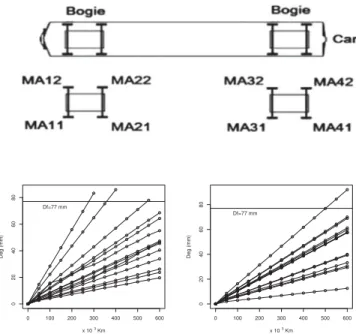
Data in Fig. 1 correspond to the train wheel degradation mea-sured in 13 equally spaced times. These data were first analyzed by [15] and [16] assuming Log-normal and Normal mixed lin-ear degradation models. Since the degradation for each wheel seems to be evolving at a constant rate, it is reasonable to as-sume linear degradation models to analyze such data. However, LN, NN, and the usual Weibull degradation models [5] may not appropriately describe the behavior of the degradation paths in this case. Depending on the wheel position in the locomo-tive (see sketch in Fig. 1), atypical degradation paths may be observed. That is the case, for instance, for wheels at position MA31. Moreover, the presence of atypical paths suggests the use of heavy tail distributions for the degradation rate. If the degradation rate is assumed to be Weibull distributed, the pa-rameters estimates may be affected by the presence of atypical paths. Consequently, quantiles for the failure time distribution or other quantities of interest that depend on these estimates are also influenced. The use of heavy tail distributions (distributions

Fig. 1. Wheels positions in the locomotive (top) and degradation paths (bot-tom) at positions MA11 (left) and MA31 (right).

which tails are heavier than the normal ones) tends to provide robust estimates for the parameters, that is, estimates that are less influenced by atypical paths. Thus, less biased estimates for the quantities of interest are also obtained under this model assumption.

For simplicity, from now on, the reciprocal degradation rate is also named degradation rate. We denote byφ(x|µ,Σ)and Φ(x|µ,Σ)the pdf and cdf of the normal distributionN(µ,Σ), respectively. If µ= 0 (respectively, µ= 0 andΣ= 1), then these functions are denoted byφ(x|Σ)and Φ(x|Σ) (respec-tively,φ(x)andΦ(x)).

II. SMSN AND LSMSN DEGRADATIONMODELS

LetYij be thejth degradation measurement for the ith

ex-perimental unit. Denote byD(tij;γ;βi)the true degradation

path of unit i at time tij, i= 1,2, . . . , n, j= 1,2, . . . , mi,

where mi is the number of measurements performed on unit

i. The general expression for the degradation model is given by Yij=D(tij;γ;βi) +εij, whereγ= (γ1, . . . , γr)t is a vector

of fixed effects which describes some common population char-acteristics,βi is the random effect related to theith unit, and

represents the individual unit characteristic andεij is the

ran-dom error associated with theith unit at timetij. There are two

model structures for linear degradation models which assume that the degradation path for theith unit are given by

D(tij;βi) =tijβ−i1 (1)

D(tij;βi) =tijβi. (2)

These two models are equivalent and the difference between them lies in the interpretation ofβi, which is the degradation

rate and the reciprocal degradation rate at unitiunder models in (1) and (2), respectively.

In degradation models, it is assumed that a failure takes place whenever the degradation path reaches a threshold,Df. The

thresholdDf is specifieda prioriby experts, usually, based on

physical characteristics of the device in study. Inference about the failure time is obtained exploring the relationship between time and degradation. If, for instance, the linear degradation path is modeled as in (1), the distribution of the failure time of unit i,Ti, is obtained considering the relationshipTi=Dfβi. This

relationship is an important tool to assess the failure fraction, the reliability, the mean time to failure or the percentile through the analytical method [11].

Different distribution forβican be assumed defining different

degradation models. The Weibull degradation model has been considered in many practical situations [5] and assumes that the random effectsβi|ς, κ∼Weibull(ς, κ),ς >0, andκ >0. This choice is, in general, motivated by the flexibility of the Weibull distribution, which provides an adequate model fit in many sit-uations. Despite its flexibility, the Weibull linear degradation model cannot be an appropriate choice in many practical situ-ations as, for instance, if the system experiences some atypical degradation paths. We develop new linear degradation models by assuming that the random effects distributions belong to the SMSN [17] and the LSMSN[18] families. Both families account simultaneously for skewness and heavy tail behaviors bringing more flexibility for the modeling.

Assuming the degradation models in (1) and lettingβi|ς, κ∼

Weibull(ς, κ), we also have a mathematically convenient model choice because, as a consequence, it follows that Ti|ς, κ∼

Weibull(ς, κ[Df]−ς). This result is particularly useful to

imple-ment the methods introduced by [5] and [11] and to determine the model structure that should be assumed, or model in (1) or in (2). Although both models in (1) and (2) are appropriate to handle degradation data with linear behavior, this closed rela-tionship between the failure time and degradation distributions does not always follow. In the following, we find the relation-ship between degradation and failure time under the proposed models.

A. Exploring the Relationship Between Degradation and the Failure Time Under the Proposed Models

Assume that the random effectβi ∼SMSN(µ, h−i1ω2, α,H)

with pdf given by

fβi|µ, hi, ω2, α = 2 ∞

0

φβi|µ, h−i1ω2

×Φ

α(βi−µ) h−i1/2ω

dH(hi|ν) (3)

where µ∈R, ω∈R+, and α∈R, respectively, the

loca-tion, scale, and skewness parameters, H(hi|ν) is a proba-bility measure defined on the sample space of the mixing random variableHandνis a vector of hyperparameters index-ingH. The mean and the variance ofβiare given, respectively,

by E[βi] =µ+

2

πk1∆, if E[H

−1/2_{]<∞, and V ar[β}

i] =

ω2_K

2−_π2k12∆2, ifE

H−1 _{<∞, where∆ =ωδ,δ=α[1 +}

α2_]−1/2 _andk

m =E[H−m /2]. The percentile of orderpof the

distribution in (3) is (βi)p =µ+ωΦSMSN−1 (p|α, hi,H), where

Φ−1

SMSN(p|α, hi,H)denotes the quantile of orderpof the

stan-dard SMSN distribution.

Proposition 1: Assume the model in (1). If βi ∼SMSN

(µ, h−_i1ω2_{, α,H), then, the failure time T}

i∼SMSN(µDf,

h−_i1ω2_D2

f, α,H).

The proof of Proposition 1 follows from (3) and (1) by notic-ing that

P(Ti ≤t|µ, ω, α, ν) = t

D f

−∞ ∞

0 2

₁

2πh−1

i ω2 1/2

×exp

−(βi−µ)

2

2h−1

i ω2

×Φ

α

βi−µ

h−12

i ω

dH(hi|ν)dβi.

As a consequence, the pdf of Ti is f(t|µ, ω, α, ν) =₀∞

2(2πh−1_ω2_D2

f)−1/2exp{−

(t−µDf)2 2h−1

i ω2D2f}Φ(

α(t−µDf)

h−

1 2

i ω Df

) dH(hi|ν),

which belongs to the SMSN family. An alternative proof for this result can be found in [17], which prove that the skew-elliptical family of distribution is closed under linear transformations.

km = (ν/2)m /2((ν−m)/2) [(ν/2)]−1. A skew-Slash

degra-dation model is obtained ifHis the beta distribution Beta(ν,1) and, in this case,km = 2ν[2ν−m]−1withν > m/2.

Addition-ally, if we assume α= 0the normal,t and slash degradation models are obtained.

Other degradation models can be built if we assume that the degradation rates have their behavior described by a distribution in the LSMSN family [18]. We say that βi∼

LSMSN(µ, h−i1ω2, α,H)if its pdf is given by

fβi|µ, hi, ω2, α = ∞

0 2 βi

φlog(βi)|µ, h−i1ω2

×Φ

α(log(βi)−µ)

h−i1/2ω

dH(hi|ν) (4)

whereµ∈R+,ω∈R+andα∈Rare, respectively, the

loca-tion, scale and skewness parameters. The functionH(hi|ν)is a probability measure defined on the sample space of the mixing random variableHandνis a vector of hyperparameters index-ingH. The family of distribution in (4) is also a shape mixture of LSN distributions which extends the shape mixture of LN distributions considered by [19].

The LSMSN family generates attractive models because it puts positive mass only on positive values, which is a more realistic assumption for degradation data. This class contains the LN family as a particular case when we setα= 0andH

is such that, almost surely,H = 1. It also recovers heavy tailed distributions putting positive mass only inR+, such as the log-t,

log-Slash, LST, and the log-skew-slash distributions.

Proposition 2: Consider the model in (1). Ifβi∼LSMSN

(µ, h−i1ω2, α,H), then, the failure time Ti∼LSMSN(µ+

log(Df), h−i1ω2Df, α,H).

The proof of Proposition 2 is similar to the one of Proposition 1. It follows from (4) and (1), for this reason omit-ted. Some properties of the LSMSN family of distribution in (4), such as marginal and conditional distributions, moments, and stochastic representations, are obtained by [18]. Proposition 2 establishes that the univariate LSMSN family of distributions is closed under linear transformations, which was not presented in [18].

This invariance condition between the degradation rate and the failure time also follows if the degradation path is D(tij;βi) =tijβiandβihas distribution in the LSMSN

fam-ily (see Proposition 3). However, the failure time distribution under such model structure does not have a closed form if the distribution ofβibelongs to the SMSN family of distributions.

Proof of Proposition 3 is similar to that of Propositions 1 and 2 thus is omitted.

Proposition 3: Consider the degradation path in (2). 1) If the degradation rate βi ∼ LSMSN(µ, h−i1ω2, α,H),

thenTi∼LSMSN(µ−log (Df), h−i1ω2,−α,H).

2) Ifβi∼SMSN(µ, h−i1ω2, α,H), then, the pdf of the failure

timeTiis given by

f(ti|µ, ω, α, ν) =

∞

0 2 t2

i

1 2πh−i1ω2D−f2

1 2

×exp

⎧ ⎪ ⎨ ⎪ ⎩−

t−_i1−µD_f−12 2h−i1ω2Df−2

⎫ ⎪ ⎬ ⎪ ⎭

×Φ

⎛ ⎝αt

−1

i −µD −1

f

h−12

i ωD−f1 ⎞

⎠dH(hi|ν)

whereµ∈ ℜ,ω∈ ℜ+ andα∈ ℜare, respectively,

loca-tion, scale, and skewness parameters,H(.|ν)is the prob-ability measure defined on the parametric space of the random variableH andνis a vector of hyperparameters indexingH.

Results in Proposition 1 to 3 are also useful to assess infor-mation about the system reliability through the classical method presented by [11] and the Bayesian method introduced by [5]. In the following, we present a data augmentation strategy to estimate the proposed degradation models and introduce a way to infer about the failure time based in its posterior predictive distribution.

B. Bayesian Inference on the Proposed Degradation Models

To estimate the degradation model, letY= (Y1, . . . ,Yn)in

whichYi= (Yi1, . . . , Yimi)

t

denotes the degradation measure-ments (path) for uniti. Letβ= (β1, . . . , βn)t be the vector of

random effects associated with thenexperimental units, where the degradation rateβiaccounts for the correlation among the

degradation measurements in the ith unit. Assume the linear degradation model given by

Yij = tijβi−1+εij,

εij|σ2

ε

iid

∼ N0;σ2

ε

(5)

fori= 1, . . . , nandj = 1, . . . , mi. Assume that, givenβand

σ2

ε, the degradation paths Y1, . . . ,Yn are independent. The

degradation measurements at uniti,Yi1, . . . , Yimi, are assumed

to be conditionally independent, givenβiandσε2.

Under these assumptions, we have thatYij|βi, σ2ε

ind

∼ N(tij

βi−1;σε2), for all i and j, and that Yi|βi, σ2ε

ind

∼ Nmi(Ψi;

σ2

εImi), where Imi denotes the identity matrix of order mi,

ti = (ti1, . . . , timi)

t _{and Ψ}

i= (ti1β−i1, . . . , timiβ

−1

i )t.

Con-sequently, the likelihood function is given by

f(Y|β, σ2

ε) = n

i= 1

⎡ ⎣

mi

j= 1

exp−_2σ12

ε

Yij−tijβi−1 2

(2πσ2

ε)1/2

⎤ ⎦.

(6) The random effects distributions are specified in the second stage of the hierarchical Bayesian modeling as their prior dis-tributions. First, assume thatβi

ind

∼ SMSN(µ, h−i1ω2, α,H).

parametrization assumed by [22], the stochastic representation for such distribution ofβiis

βi=d µ+ ∆Ui+Hi−1/2τ1/2U1i, where∆ =ωδ,δ=α(1 +

α2₎−1/2_{, τ=1−δ}2_ω2_{, U}

i=Hi−1/2|U0i|, U1i d

=U0i

ind

∼

N(0,1)andHiis a random variable with probability measure Hindexed by the parameter vectorν.

The distribution of βi can be hierarchically rewritten as

follows:

βi|Ui=ui, Hi =hi

ind

∼ Nµ+ ∆ui, h−i1τ

, Ui|Hi=hi ind∼ N0, h−i1

1{ui>0},

Hi

iid

∼ H(hi|ν).

⎫ ⎪ ⎬ ⎪ ⎭ (7)

Hereby,1{A} is the indicator function of eventAand=d de-notes equal in distribution. The variable Ui is nonobservable

and should be estimated. Consequently, we should obtain the posterior distribution for the vector of parametersθ= (β, σ2

ε,

U, H, µ,∆, τ). Assume thatσ2

ε, U,H, µ,∆, andτ are,a

priori, independent and that

σ2

ε ∼IG(rσ2

ε, sσ2ε), µ∼N(m, V), ∆∼N(µ∆, σ∆), τ ∼IG(rτ, sτ)

#

(8)

where IG(a, b),a >0,b >0, is the IG with meanb(a−1)−1_if

a >1.

To sample from the posterior distributions, we develop an algorithm based on both Markov chain Monte Carlo (MCMC) methods and the data augmentation technique previously de-scribed. One advantage of using the stochastic representation in (7) is that we obtained closed forms for almost all posteriorfcd simplifying the posterior sampling process.

Proposition 4: For the degradation model in (5) and the prior specifications in (7) and (8), the posterior fcd for(β, σ2

ε,U, µ,

∆, τ)are

βi|θ−βi,Y∝ exp

⎧ ⎨ ⎩−

1 2σ2

ε mi

$

j= 1

Yij−

tij

βi 2

−hi

2τ [βi−(µ+ ∆ui)]

2

⎫ ⎬ ⎭

σε2|θ−σ2

ε,Y∼ IG

_n

$

i= 1

mi

2 +rσε2, 1

2

n $

i= 1

mi

$

j= 1

Yij−

tij

βi 2

+sσ2

ε

⎞ ⎠

Ui |θ−Ui,Y∼ N

∆ (βi−µ)

∆2_+τ ,

τ h−i1

∆2_+τ

1{ui>0}

µ|θ−µ,Y∼ N ⎛ ⎝

$n

i= 1(βi−∆ui)V

∗ i +mτ

n i= 1h

−1

i $n

i= 1V

∗ i +τ

n i= 1h

−1

i

V τn

i= 1h

−1

i $n

i= 1V

∗ i +τ

n i= 1h

−1

i ⎞ ⎠

∆|θ−∆,Y∼ N

⎛ ⎝σ

2 ∆

$n

i= 1(βi−1)U

∗ i +µ∆τ

n i= 1h

−1

i

σ2∆

$n i= 1U

∗ i +τ

n i= 1h

−1

i

σ2 ∆τ

n i= 1h

−1

i

σ2 ∆

$n i= 1U

∗ i +τ

n i= 1h

−1

i ⎞ ⎠

τ |θ−τ,Y∝ IG

n 2 +rτ,

n $

i= 1

[βi−(µ+ ∆ui)]2

2h−i1

+sτ

whereV∗ i =V

%

k=ih−k1,Ui∗=ui%k=ih−k1.

IfHis a degenerated distribution putting all probability mass in 1, then the posterior full conditional distribution of all param-eters are given in Proposition 4 assuminghi= 1for alli. IfH

is the Gamma(ν/2, ν/2)distribution andνhas a Jeffreys prior distribution such that

π(ν)∝

_ν

ν+ 3

1 2

∂2_logΓν

2

∂ν2

∂2_logΓν+ 1 2

∂ν2 −

2 (ν+ 3) ν(ν+ 1)2

1 2

(9)

then the sampling scheme given in Proposition 4 is completed by considering the posterior fcd for hi and ν given,

respe-ctively, by

hi|θ−hi,Y∼IG

ν 2 + 1,

[βi−(µ+ ∆ui)]2

2τ +

u2 i 2 + ν 2

ν|θ,Y∝ & ν

2

ν

2

Γ(ν₂)

'_{n n}

i= 1

&

1 hi

ν

2+ 1'

×

ν ν+ 3

1 2 exp − n $

i= 1

ν 2hi

×

∂2_logΓν

2

∂ν2

∂2_logΓν+ 1 2

∂ν2 −

2 (ν+ 3) ν(ν+ 1)2

1 2

.(10)

The prior distribution forν given in (9) is the independent Jeffreys prior introduced by [25] for T linear regression model. Such prior is a proper distribution that has been successfully used to estimateνin different T models. Samples of the posterior distributions ofσ2

ε,U,H, µ,∆, andτ can be obtained using

the Gibbs sampling algorithm. To sample from the posterior full conditional distributions ofν andβ, the Metropolis–Hastings algorithm can be considered. The representation in (7) greatly facilitates the inference in the proposed degradation model since it also allows us to use the WinBUGS.

If βiind∼ LSMSN(µ, h−i1ω, α,H), the inference can be

done using a similar strategy. In this case, it follows that log(βi)∼SMSNµ, h−1ω2, α,H. Consequently, we can

con-sider that log(βi) d

ωδ, δ=α[1 +α2_]−1/2_{, τ=1−δ}2_ω2_{, U}

i=Hi−1/2|U0i|,

U1i d

=U0i

ind

∼ N(0,1)andHiis a random variable with

proba-bility measureHindexed by the parameter vectorν. It follows that the distribution ofβiis

log(βi)|Ui=ui, Hi=hi∼Nµ+ ∆ui, h−i1τ

(11)

whereUiandHiare defined as in (7).

Proposition 5: For the degradation model in (5) and the prior specifications in (11) and (8), the posterior fcd for(β, σ2

ε,U,

µ,∆, τ)are

log(βi)|θ−βi,Y∝exp

⎧ ⎨ ⎩−

1 2σ2

ε mi

$

j= 1

Yij−

tij

log(βi) 2

−hi

2τ [log(βi)−(µ+ ∆ui)]

2

σ2

ε|θ−σ2

ε,Y∼IG

_n

$

i= 1

mi

2 +rσ2ε 1

2

n $

i= 1

mi

$

j= 1

Yij−

tij

log(βi) 2

+sσ2

ε

⎞ ⎠

Ui|θ−Ui,Y∼N

_{∆ (log(β} i)−µ)

∆2_+τ ,

τ h−i1

∆2_+τ

1{ui>0}

τ|θ−τ,Y∝IG

n

2 +rτ, sτ+

n $

i= 1

[log(βi)−µ−∆ui]2

2h−1

i

µ|θ−µ,Y∼N ⎛ ⎜ ⎜ ⎜ ⎜ ⎝ $n

i= 1(log(βi)−∆ui)V

∗ i +mτ

n i= 1h

−1

i $n

i= 1V

∗ i +τ

n

i= 1

h−1

i

V τn

i= 1h

−1

i $n

i= 1V

∗ i +τ

n i= 1h

−1 i ⎞ ⎟ ⎟ ⎟ ⎟ ⎠

∆|θ−∆,Y∼N

⎛ ⎝σ

2 ∆

*$n

i= 1(log(βi)−1)U

∗ i + σ2 ∆ $n i= 1U

∗ i +τ

n i= 1h

−1

i

+µ∆τ

n i= 1h

−1

i

σ∆2

$n i= 1U

∗ i +τ

n i= 1h

−1

i

σ∆2τ

n i= 1h

−1

i

σ∆2

$n i= 1U

∗ i +τ

n i= 1h

−1

i ⎞ ⎠

whereV∗

i =V%k =ih −1

k ,Ui∗=ui%k =ih −1

k .

As previously discussed, if H is a degenerate distribution putting mass in 1, then the posterior fcd of all parameters are given in Proposition 5 replacinghi by 1 for all i. IfHis the

Gamma(ν/2, ν/2)distribution and the prior distribution ofνis given in (9), then the posterior fcd forνis given in (10) and for hiit is given by

hi|θ−hi,Y∼IG

ν 2+1,

[log(βi)−(µ+ ∆ui)]2

2τ +

u2 i 2 + ν 2 .

C. Posterior Predictive for the Failure Time

To assess the system reliability, we consider the posterior pre-dictive distribution of the future failure time. LetTn+ 1andYn+ 1

be the failure time and the degradation path of a new unit, respec-tively. Assume that it is independent of the observed units. As-suming the degradation model in (1), the cumulative distribution ofTn+ 1, given the degradation measuresY= (Y1, . . . ,Yn),

is given by

FTn+ 1|Y,Yn+ 1(t) = fβ,βn+ 1|y,yn+ 1(β, βn+ 1)

P(βn+ 1Df ≤t|yn+ 1, βn+ 1)dβn+ 1dβ

=

βn+ 1≤_{D f}t

fβn+ 1|y,yn+ 1(βn+ 1)dβn+ 1

=Fβn+ 1|y,yn+ 1(tD

−1

f ). (12)

To infer aboutTn+ 1it is necessary to find the posterior

distri-bution ofβn+ 1|Y,Yn+ 1 for which we need, at least, the initial

degradation of the new unit. Since the degradation information about the new unit andYn+ 1 is in general not available, it is

in-cluded in the likelihood as a latent data. Samples of the posterior distributions ofβn+ 1,Yn+ 1 and the other parameters are

ob-tained assuming the following augmented likelihood function:

f(Y,Yn+ 1|β, βn+ 1, σ2ε) = n+ 1

i= 1

mi

j= 1

₁

2πσ2

ε 1/2

×exp

− 1

2σ2

ε

Yij−tij

βi 2

(13)

where mn+ 1 = 1. It can be proved that the posterior full

conditional distribution for the latent degradationYn+ 1,1is

Yn+ 1,1|Y,β, βn+ 1, σε2 d

=Yn+ 1,1 ∼N

tn+ 1,1

βn+ 1,1

, σε2

.

The posterior full conditional distribution for the other param-eters are obtained as shown in Section II-B. Samples of the posterior predictive distribution ofTn+ 1 are obtained from the

posterior sample ofβn+ 1 by assuming the model relationship

between the failure time and the degradation which is, under model in (1), given by D=T /β. Posterior summaries of Tn+ 1, such as the mean time to failureE[Tn+ 1|Y,Yn+ 1], the

reliabilityRTn+ 1|Y,Yn+ 1(t)and the percentiles of the posterior

summarizing the generated sample. Similar strategy can be used for the degradation model in (2). (See [9] and [14] for a different approach.)

As an alternative procedure, results in Proposition 1 to 3 can be considered to obtain E[Tn+ 1|Y] and RTn+ 1|Y(t)

as follows. It can be proved FTn+ 1|Y(t) =Eθζ|Y(FTn+ 1|θζ (t)), RTn+ 1|Y(t) =Eθζ|Y

RTn+ 1|θζ(t)

, and E[Tn+ 1|y] =

Eθζ|Y

ETn+ 1|θζ (t)

, whereθζ denotes the parameters in the

prior model for failure times. These results prove that the method introduced by [5] to obtain the fraction of failure, the mean fail-ure time and the reliability is valid. If a posterior sample ofθζ

and, for instance, the closed expression for the reliability given θζare available, we can use the plug-in method in order to

ob-tain a posterior sample ofRTn+ 1|θζ(t). Averaging this sample,

we obtainRTn+ 1|Y(t). Details can be found in [5]. To obtain

the posterior quantiles of the distribution ofTn+ 1, the method

considered by [5] can not be applied. There is not a linear re-lationship between the quantiles of the distributions ofTn+ 1|Y

andTn+ 1|θζand, because of this, some inconsistent results can

be obtained by using Hamada’s approach. See Section III for a comparison of Hamada’s and the proposed method.

D. Model Selection in Degradation Models

For model comparison, we consider the LPML, DIC, BF, and WAIC (for a review see [26]). The LPML, DIC, BF, and WAIC are calculated based on both degradation and PFT obtained by the approximated method [11]. The LPML for degradation model is calculated using two approaches: assuming each degra-dation measureYij(LPML) and the complete degradation path

Yi(LPML*).

To calculate the DIC, letD=−2 log (f(x|θ)) be the de-viance and denote byD¯ the posterior mean ofD. Assume that

ˆ

D=−2 log (f(x|ˆθ)), in whichθˆis some posterior estimate of θ. LetpD= ¯D−Dˆ. The DIC is defined as

DIC= ¯D+pD= ˆD+ 2pD= 2 ¯D−D.ˆ (14)

A small value for the DIC indicates a better model. We as-sume that ˆθ is the posterior mean of θ. However, posterior modes and medians can also be used. Despite its popularity, the DIC usually fails in selecting models that includes latent variables [27].

The LPML is calculated from the conditional predictive ordi-nate (CPO), which allows us to assess goodness of fit as well as to perform model comparisons. For the observationithe CPO is defined as the predictive distribution ofxi given the other

observations in the sample, that is, CPOi=f(xi|x(−i)). If a

sampleθ(l)_{,l= 1, . . . , L, of the posterior distribution of θis}

available, an approximation for the CPOiis given by

,

CPOi= &

1 L

L $

l= 1 1 fxi|θ(l)

'−1

. (15)

The information the CPOi brings about the model fit can be

summarized using the statistics LPML=n−1-n

i= 1log (CPOi)

in whichnis the sample size. A high value for LPML indicates a good model.

The BF measures the evidence in favor of a modelM1if

com-pared to another modelM2. It is defined as the ratio between the

predictive distributions obtained under the models under com-parison, that is, BF=f1(x)/f2(x). The predictive distributions

can be estimated by

fi(x) =

&

1 L

L $

l= 1 1 fx|θ(l)

'−1

(16)

whereθ(l) _{is as defined before. A high value for the BF brings}

evidence in favor ofM1.

[28] defined the widely applicable information criterion (WAIC) as

WAIC∗=

n $

i= 1 log

&

1 L

L $

l= 1

fxi|θ(l)

'

−pWAIC

where, in this paper, the penalty pWAIC=-ni= 1[Var(logf (xi|θ))]and Var is the sample variance. According to this cri-terion, the highest the WAIC∗, the best the model. WAIC∗and DIC produces similar results if a scale modification in which WAIC=−2WAIC∗is considered. A small value for WAIC indi-cates a better model fit. We consider WAIC for the comparisons in next sections.

To obtain information about the model fit, we can con-sider the original degradation data or the PFT obtained through the degradation paths. However, to consider the PFT data [11], it is necessary to obtain the failure time distri-bution induced by the degradation model. For the robust models introduced in Section II we obtained a closed form for such distribution in almost all cases. Using these ap-proaches, the likelihood functionf(x|θ)in the previous ex-pressions must be replaced by f(xi|θ) =f(yi|θ,y[−yi]) =

mi

j= 1(2πσ 2

ε)−1/2exp{−

1 2σ2

ε

[yij−D(tij;βi)]2},ifyi is the

degradation path for uniti, or byf(xi|θ) =fti|θ,t[−ti]_if

we consider the PFT, in whichfti|θ,t[−ti]_{is the failure time}

distribution induced by the degradation model, that is, by the prior distribution we assume for the degradation rate. We can also calculate all these statistics considering the degradationyij

of an unitiat timej. In this case

f(xi|θ) =fyij|θ,y[−yi j]

= 2πσε2 −1/2

exp

. − 1

2σ2

ε

[yij−D(tij;βi)]2 #

.

(17)

III. ANALYSIS OFARTIFICIALDATA

The goal, in this section, is to infer about the failure time of a new unit considering artificial data. Proposed degradation models are fitted and compared with the widely used Weibull degradation model. Estimates for the new unit failure time ob-tained assuming the posterior predictive distribution and the Hamada’s method are also compared.

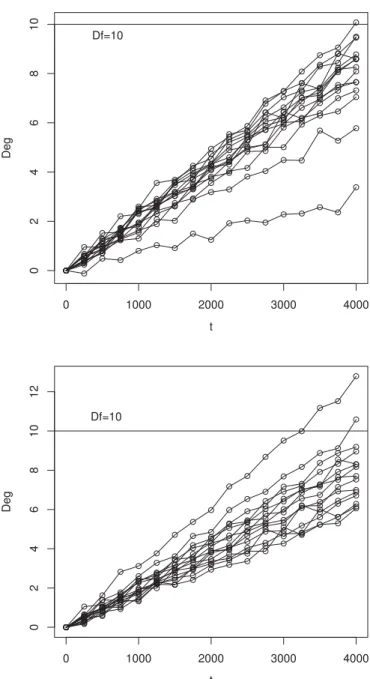
Fig. 2. Degradation paths for scenarios D-LST (top) and D-W (bottom).

distributions whenever the degradation rates have distributions in both classes, the SMSN and LSMSN families.

Data are generated assumingn= 15independent units which are observed for a total time of 4.000 hours. The degradation is measured atmi= 17equally spaced time intervals. The errors

are independent and normally distributed with varianceσ2

ǫ =

0.04. The initial degradation yi0 is zero for all units and the

failure threshold isDf = 10. Two scenarios are considered. In

the scenario named D-LST, we assume thatβi iid

∼LST6; 0.22; 10; 4). In the second scenario, named D-W, we assume that βi

iid

∼Weibull6; 550−6_.

To analyze the generated data (see Fig. 2), we fit Weibull and models belonging to the proposed class of degradation models. Specifically, we fit N,t, LN, log-t, SN, ST, LSN, and LST degra-dation models. Some of these proposed models are heavy-tailed

TABLE I

GEWEKE’SSTATIONARITYTEST ANDBROOKS, GELMAN ANDRUBIN POTENTIALSCALEREDUCTIONFACTOR FORCONVERGENCEASSESSMENT,

LST MODEL ANDD-LST SCENARIO

Parameter Geweke PSRF

Chain 1 Chain 2 Chain 3

µ −1.64 −0.88 1.10 1.00 ω2 _{1.72 0.08 −1.23 1.00}

δ 1.32 −0.53 0.08 1.00

ν 1.15 −1.58 −0.88 1.01 β1 6 1.56 −1.00 −0.88 1.02

and can be more appropriate to analyze data in scenario D-LST which presents atypical paths. Because they are robust models, they should also provide good model fit to data in D-W sce-nario. To mimic the case study, we assume that there is not any prior information about the parameters by eliciting the follow-ing flat prior distributions:σ2

ε ∼IG(10−3,103),µ∼N(0,106),

∆∼N(0,106_),τ∼IG(10−3_,103_{),ς∼Gamma(10}−3_,10−3₎

andκ∼Gamma(10−3_,10−3_{), whereςandκare the parameters}

indexing the Weibull distribution.

For the MCMC, we run a chain of size 220 000 000. Af-ter the convergence has been attained, we discarded the first 100 000 000 as the burn-in period and considered a lag of 60000 steps to avoid correlation. A posterior sample of size 2000 was obtained. The algorithm was implemented using WinBUGS 1.4 software and R 3.1.0 [29] was considered to summarize the posterior results.

Table I shows the results related to the MCMC stationarity and convergence assessment for the main parameters of LST fit to D-LST data. For this purpose, we consider the criteria introduced by [30]–[32]. The results correspond to 3 chains of size 2000. For Geweke’s stationarity test the fraction in 1st window is 0.1 and in 2nd window is 0.5. The Geweke’s values are all between−1.96 and 1.96 indicating that the chain reached stationarity. The PSRF for convergence assessment are up to 1.1 for all parameters. Consequently, stationarity and convergence are achieved for LST adjustment. Similar results were observed for all other scenarios and parameters and thus were omitted.

A. Inference for the Failure Time

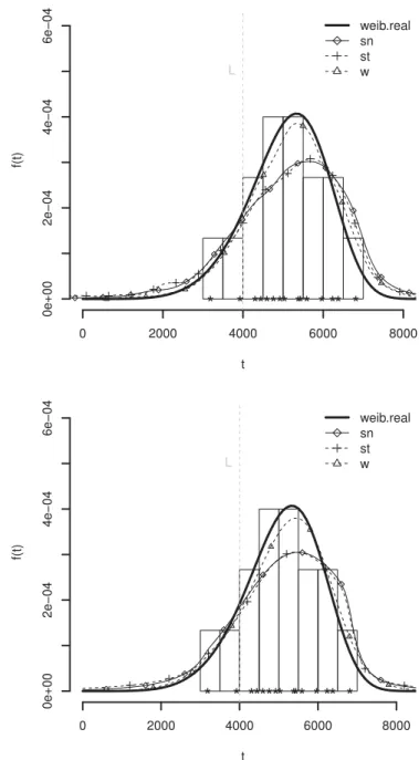
Fig. 3. Histogram of the PFT, the true (solid line) and the posterior pdf of a new unit failure time assuming the posterior predictive (top) and Hamada’s method (bottom), data D-LST. The vertical dotted line represents the study time.

Table II shows the percentiles of order 1%, 5%, 95%, and 99% of the posterior predictive distribution of Tn+ 1.

It also presents the posterior mean for the percentiles of same order of the distribution of Tn+ 1, given θ, and the

LB and UB bounds of the 95% HPD interval of such percentiles provided by Hamada’s method. For scenario D-LST, the true percentiles of order1%,5%,95%, and99%are, respectively, 3963.69, 4067.97, 7029.52, and 10131.49. The centiles for the empirical distribution of the PFT (empirical per-centiles) are 4071.11, 4161.96, 8648.00, and 12434.99, respec-tively. For scenario D-W, the true percentiles of order1%,5%, 95%and99%are, respectively, 2555.01, 3352.53, 6603.59, and 7094.20, and the empirical percentiles equals 3290.52, 3703.24, 6507.93, and 6753.31, respectively. We underlined the most bi-ased estimates. In bold style, we present the results provided by

Fig. 4. Histogram of the PFT, the true (solid line) and the posterior pdf of a new unit failure time assuming the posterior predictive (top) and Hamada’s method (bottom), data D-W. The vertical dotted line represents the study time.

models which estimated pdf better approach the true one based on a visual graphic analysis only.

TABLE II

PERCENTILES FOR THEFAILURETIMEDISTRIBUTIONUSING THEPOSTERIOR PREDICTIVEDISTRIBUTION ANDHAMADA’SMETHOD

FORALLMODELS, SCENARIOSD-LSTANDD-W

LN models are comparable when analyzing Weibull data. By using Hamada’s method, we also have the posterior distribution for the prior quantiles ofTn+ 1|θ. If, for instance, the LST model

is fitted to the D-LST data, the prior percentile of5%ofTn+ 1|θ

is between 2788.09 and 4375.21 with posterior probability of 0.95. However, this interval does not measure the posterior un-certainty about the5%quantile of the distribution for the failure time of a future unitTn+ 1, as suggested in [5].

B. Selecting a Model

Table III shows the ordination from the best to the worst models, for all datasets, according to the criteria presented in Section II-D. It also presents the well-known Kolmogorov– Smirnov statistics (KS-EMP) comparing the estimated Proposed and Hamada’s method and empirical cdf of the PFT. Consider-ing the criteria calculated usConsider-ing the degradation data, we noticed that the LPML* was inefficient for model selection, mainly for data generated from light tailed distribution (D-W). In this case, the true model was pointed out as the worst model. LPML, DIC, and WAIC identified correctly the LST model for D-LST dataset but failed for D-W. For D-W these three criteria indicate the LSN as the best model. The BF correctly selected the W in scenario D-W.

Based on the PFT, the LPML had the best performance se-lecting the correct models in both cases, and DIC works well only for D-W scenario. WAIC and the BF have not selected the correct model for both datasets. Although DIC and WAIC do

TABLE III

MODELCOMPARISON, SIMULATEDDATASET

TABLE IV

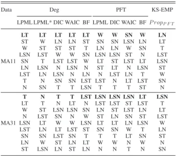
MODELCOMPARISON INTRAINWHEELDEGRADATIONDATA

Data Deg PFT KS-EMP

LPML LPML* DIC WAIC BF LPML DIC WAIC BF P ropP F T

LT LT LT LT LT W W SN W LN

ST W LN LN ST SN SN LSN LN LT

W ST ST ST T LN LN W SN T

LSN LST W W SN LSN LSN ST N LST

MA11 SN T LST LST W LT ST LST LT LSN

LN LSN N LSN N ST LT N LSN ST

LST LN LSN N LN N LST LN T W

T N SN SN LST LST N LT LST SN

N SN T T LSN T T T ST N

T N T T LST LSN LSN LSN LT LSN

LT T N LT N LST LST ST LST T

W ST LSN LSN SN LN ST LST LN LT

N LST SN N W ST LN SN ST LST

MA31 LSN LT W W LSN LT LT LN LSN W

LST LN LT LST ST SN SN W T LN

SN SN LST SN T T T LT SN ST

LN W ST LN LT W W N W N

ST LSN LN ST LN N N T N SN

not have a good performance when analyzing data in scenario D-LST, they select a heavy tailed model to fit the data. According to all criteria, the Weibull degradation model is always among the worst models when the dataset follows a LST distribution. Moreover, the criteria based on degradation data (respectively, PFT) have better performance when data was generated from LST (Weibull) distribution.

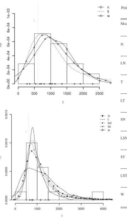
Fig. 5. PFTs histogram and the posterior predictive distribution of a new unit failure time for train wheels at positions MA11 (top) and MA31 (bottom).

and it is the third best for scenario D-LST. The widely used W, LN, and N degradation models are among the worst models for data in scenario D-LST presenting high distance from the true cdf. According to this criterion, the W degradation model has poor performance, including when considered to analyze data in scenario D-W .

IV. CASESTUDY: TRAINWHEELDEGRADATIONDATA

Data reported in [15] and [16] are analyzed assuming the proposed degradation models. A sample of 14 locomotives is considered. Data correspond to the train wheel degradation. Degradation is the amount of wear (in mm) at each inspection timet(i.e., initial diameters minus diameter measured at time t). It is measured in 13 equally spaced timest0 = 0km,t1 =

TABLE V

PERCENTILES FOR THEFAILURETIMEPOSTERIORPREDICTIVEDISTRIBUTION FORALLMODELS ANDMA11ANDMA31 WHEELS

Model MA11 MA31

perc. Empirical Post. pred Empirical Post. pred

t1 286.49 −410.42 519.91 −1059.70

N t5 328.33 5.39 600.99 −307.75

t9 5 2046.03 2103.87 2245.13 2513.36

t9 9 2244.72 2596.78 3288.65 3119.49

t1 286.49 168.75 519.91 256.14

LN t5 328.33 309.05 600.99 385.67

t9 5 2046.03 2827.94 2245.13 2559.36

t9 9 2244.72 5060.56 3288.65 4256.20

t1 286.49 −1317.65 519.91 −5255.78

T t5 328.33 −186.51 600.99 −262.66

t9 5 2046.03 2247.86 2245.13 2177.37

t9 9 2244.72 3879.54 3288.65 10463.99

t1 286.49 80.07 519.91 86.39

LT t5 328.33 261.95 600.99 392.22

t9 5 2046.03 3394.97 2245.13 2551.90

t9 9 2244.72 15881.56 3288.65 12483.47

t1 286.49 −176.91 519.91 205.57

SN t5 328.33 200.30 600.99 444.24

t9 5 2046.03 2398.20 2245.13 2798.76

t9 9 2244.72 3257.95 3288.65 3475.88

t1 286.49 116.08 519.91 338.40

LSN t5 328.33 226.68 600.99 480.95

t9 5 2046.03 2635.98 2245.13 2870.60

t9 9 2244.72 5109.00 3288.65 5257.29

t1 286.49 −429.29 519.91 202.17

ST t5 328.33 186.78 600.99 483.28

t9 5 2046.03 2906.79 2245.13 3253.44

t9 9 2244.72 6860.53 3288.65 11485.55

t1 286.49 34.85 519.91 274.32

LST t5 328.33 188.80 600.99 483.71

t9 5 2046.03 2804.11 2245.13 4317.54

t9 9 2244.72 8447.44 3288.65 39868.21

t1 286.49 107.11 519.91 50.96

W t5 328.33 257.25 600.99 207.03

t9 5 2046.03 2260.30 2245.13 2716.37

t9 9 2244.72 2927.77 3288.65 3680.62

50 000 km,. . . , t13=600 000 km. A failure occurs when the

wheel degradation reaches the threshold levelDf =77 mm.

Table III shows that the LMPL and DIC based on the PFT selected the correct model for light tailed data and LMPL, DIC, and WAIC calculated assuming the degradation data indicated correctly the model in the heavy tail scenario. Since MA11 data has light tail behavior and MA31 data behave as a heavy tail data, taking these criteria into consideration we conclude that Weibull and T degradation models are, respectively, the best for MA11 and MA31 data (see Table IV). The pdf for a new unit failure time distribution obtained under such models are exhibited in Fig. 5 joint with the ones that provided the best approximations for the empirical distribution based on a visual graphic analysis. The empirical pdf is built using the PFT. Table IV shows the ordination from the best to the worst model, for all datasets, according to all criteria. All models are comparable to analyze MA11 data. They provided very similar pdf with a smooth difference in favor of the W and LT models. The LT (respectively, W) degradation model is pointed out as the best model by five (respectively, three) criteria. ST, LSN, LST, LT, and LN degradation models better fitted to MA31 dataset providing a good approximation to the empirical curve. For this data, four criteria selected the LSN model as the best and three others indicate model T.

Table V presents the percentiles of order1%,5%,95%, and 99%under all models, for wheels at position MA11 and MA31. To the analysis, consider only the models selected as the best by the most of criteria which, respectively, are LT and LSN for datasets MA11 and MA31. Based on these models, we for instance conclude that5%of the train wheels at position MA11 and M31 will degrade beyond the threshold of 77 mm before 261.95×103_{Km and480.95×10}3_{, respectively.}

V. CONCLUSION ANDFUTUREWORKS

We introduced classes of linear degradation models that are able to accommodate skewness and heavy-tailed behavior. We assumed that the degradation (reciprocal degradation) rate has distribution in both the SMSN and LSMSN families of distri-butions. We proved that the failure time distribution belongs to the same family as the degradation rate for the majority of the proposed models, which is particularly useful to implement the methods introduced by [5] and [11]. We presented a data augmentation algorithm to sample from the posterior distribu-tions. We also proposed a strategy to infer about the failure time through the predictive distributions and showed the incon-sistence in Hamada’s approach to obtain the quantiles of the failure time distribution. The proposed models were compared with the Weibull degradation model using simulated datasets. Additionally, we analyzed the train wheel degradation data.

The proposed degradation models are competitive models. They presented very good performance when analyzing data that present outliers, heavy tails and skewness behaviors being better than the Weibull degradation model. Their performances are comparable to the W when analyzing light-tailed and symmetric data.

The proposed models showed to be a reasonable option to analyze the train wheel degradation data, mainly because the

degradation paths in some positions have strong asymmetry and outliers.

Methods for model comparison based on degradation and PFT data were discussed. LPML, DIC, and WAIC based on degradation data and the Kolmogorov–Smirnov distance based on the PFT selected the true model whenever data were gen-erated from heavy tailed distribution. LPML, DIC, and WAIC based on PFT data and the BF worked better if data were gen-erated from Weibull and LST distributions. However, because we only run one simulated sample in each scenario, the study presented in this paper is not conclusive about the best method for model selection in degradation data. Much effort must be still done in finding an efficient method for model selection in degradation data when dealing with Bayesian approach.

ACKNOWLEDGMENT

The authors would like to thank the Editors and two anony-mous referees whose comments and suggestions lead to a im-proved paper. The authors also gratefully acknowledge CNPq (Conselho Nacional de Desenvolvimento Cient´ıfico e Tec-nol´ogico) of the Ministry for Science and Technology of Brazil and FAPEMIG (Fundac¸˜ao de Amparo `a Pesquisa do Estado de Minas Geraisfor a partial allowance to their researches. It was developed when the first author was a Ph.D. student at the Department of Statistics, UFMG.

REFERENCES

[1] C. J. Lu and W. Meeker, “Using degradation measurements to estimate a time-to-failure distribution,”Technometrics, vol. 35, no. 2, pp. 161–174, May 1993.

[2] C. J. Lu, W. Meeker and L. Escobar, “A Comparison of degradation and failure-time analysis methods for estimating a time-to-failure distribution,”

Statistica Sinica, vol. 6, no. 3, pp. 531–546, Jul. 1996.

[3] J. Lu, J. Park and Q. Yang, “Statistical inference of a time-to-failure distribution derived from linear degradation data,”Technometrics, vol. 39, no. 4, pp. 391–400, Nov. 1997.

[4] M. Robinson and M. Crowder, “Bayesian methods for a growth-curve degradation model with repeated measures,”Lifetime Data Anal., vol. 6, no. 4, pp. 357–374, Dec. 2000.

[5] M. Hamada, “Using degradation data to assess reliability,”Quality Eng., vol. 17, no. 4, pp. 615–620, 2005.

[6] V. R. B de Oliveira and E. A. Colosimo, “Comparison of methods to estimate the time-to-failure distribution in degradation tests,”Quality Rel. Eng. Int., vol. 20, no. 4, pp. 363–373, Jun. 2004.

[7] S. Liu . and W. Meeker, “Using degradation models to assess pipeline life,” Iowa State Univ., Ames, IA, USA, Tech. Rep. 127, Oct. 2014. [Online]. Available: http://lib.dr.iastate.edu/stat_las_preprints/127/

[8] K. Doksum, “Degradation rate models for failure time and survival data,”

CWI Quart., vol. 4, pp. 195–203, 1991.

[9] J. Lawless and M. Crowder, “Covariates and random effects in a gamma process model with application to degradation and failure,”Lifetime Data Anal., vol. 10, pp. 213–227, Sep. 2004.

[10] X. Wang and D. Xu, “An inverse Gaussian process model for degradation data,”Technometrics, vol. 52, no. 2, pp. 188–197, May 2012.

[11] W. Meeker and L. Escobar,Statistical Methods for Reliability Data, 1st ed. New York, NY, USA: Wiley, 1998.

[12] M. S. Nikulin, N. Limnios, N. Balakrishnan, W. Kahle and C. Huber-Carol,Advances in Degradation Modeling, 1st ed. New York, NY, USA: Birkhuser, 2010.

[13] P. Lim, C. K. Goh, K. C. Tan, and P Dutta, “Multimodal degradation prognostics based on switching Kalman filter ensembler,”IEEE Trans. Neural Netw. Learn. Syst., vol. 28, no. 1, pp. 136–148, Jan. 2017. [14] T. Yuan and J. Yizhen, “A hierarchical Bayesian degradation model for

[15] M. A. Freitas, M. L G Todedo, E. A. Colosimo, and M. C. Pires, “Us-ing degradation data do assess reliability: A case study on train wheel degradation,”Quality Rel. Eng. Int., vol. 25, n. 5, pp. 607–629, Jul. 2009. [16] J. C. Ferreira, M. A. Freitas, and E. A. Colosimo, “Degradation data analysis for samples under unequal operating conditions: A case study on trains wheels,”J. Appl. Statist., vol. 39, n.12, pp. 2721–2739, Sep. 2012. [17] M. D. Branco and D. K. Dey, “A general class of multivariate

skew-elliptical distributions,”J. Multivariate Anal., vol. 79, no. 1, pp. 99–113, Oct. 2001.

[18] Y. V. Marchenko, M. G Genton, “Multivariate log-skew-elliptical distri-butions with applications to precipitation data,”Environmetrics, vol. 21, no. 3/4, pp. 318–340, Apr. 2010.

[19] C. A. Vallejos and M. F. J. Steel, “Objective Bayesian survival analysis using shape mixtures of log-normal distributions,”J. Amer. Statist. Assoc., vol. 110, no. 510, pp. 697–710, Jan. 2015.

[20] D. A. van Dyk and X. L. Meng, “The art of data augmentation,”J. Comput. Graph. Statist., vol. 10, no. 1, pp. 1–50, Mar. 2001.

[21] C. S. Ferreira, H. Bolfarine and V. H. Lachos, “Skew scale mixtures of normal distributions: Properties and estimation,”Statist. Methodol., vol. 8, no. 2, pp. 154–171, Mar. 2011.

[22] V. G. Cancho, D. K. Dey, V. H. Lachos, and M. G. Andrade, “Bayesian nonlinear regression models with scale mixtures of skew-normal distribu-tions: Estimation and case influence diagnostics,”Comput. Statist. Data Anal., vol. 55, no. 1, pp. 588–602, Jan. 2011.

[23] A. Azzalini, “A class of distributions which includes the normal ones,”

Scandinavian J. Statist.,vol. 12, no. 2, pp. 171–178, 1985.

[24] N. Henze, “A probabilistic representation of the ’skew-normal’ distribu-tion,”Scandinavian J. Statist.,vol. 13, no. 4, pp. 271–275, 1986. [25] T. C. O. Fonseca, M. A. R. Ferreira, and H. S. Migon, “Objective Bayesian

analysis for the Student-t regression model,”Biometrika, vol. 95, no. 2, pp. 325–333, Jun. 2008.

[26] A. Gelman, J. Hwang, and A. Vehtari, “Understanding predictive in-formation criteria for Bayesian models,”Statist. Comput., vol. 24, n. 6, pp. 997–1016, Nov. 2014.

[27] G. Celeux, F. Forbes, C. P. Robert, and D. M Titterington, “Deviance information criteria for missing data models,” Bayesian Anal., vol. 1, no. 4, pp. 651–674, Jan. 2001.

[28] S Watanabe, “Asymptotic equivalence of Bayes cross validation and widely applicable information criterion in singular learning theory,”J. Mach. Learn. Res., vol. 11, no. 1, pp. 3571–3594, Dec. 2010.

[29] R Core Team, “R: A Language and Environment for Statistical Com-puting,” R Foundation for Statistical Computing, Vienna, Austria, 2014. [Online]. Available: http://www.R-project.org/

[30] J. Geweke, “Evaluating the accuracy of sampling-based approaches to calculating posterior moments.,” inBayesian Statistics 4, J. M. Bernardo, J. O. Berger, A. P. Dawid, and A. F. M. Smith, Eds. Oxford, U.K.: Clarendon, 1992.

[31] A. Gelman and D. B. Rubin, “Inference from iterative simulation using multiple sequences (with discussion),”Statist. Sci., vol. 7, no. 4, pp. 457– 511, 1992.

[32] S. P. Brooks and A. Gelman, “General methods for monitoring conver-gence of iterative simulations,”J. Comput. Graph. Statist.,vol. 7, no. 4, pp. 434–455, 1998.

Rivert P. B. Oliveirareceived the B.Sc. and Ph.D. degrees in statistics from the Federal University of Minas Gerais, Belo Horizonte, Brazil, in 2008 and 2015, respectively, and the M.Sc. degree in produc-tion engineering from the same instituproduc-tion in 2011.

He is an Adjunct Professor at Federal University of Ouro Preto, Ouro Preto, Brazil. His research interests include reliability, industrial statistics, and Bayesian inference.

Rosangela H. Loschireceived the B.Sc. and Ph.D. degrees in statistics from the University of S˜ao Paulo, Brazil, in 1992 and 1998, respectively.

She is a Full Professor at Federal University of Minas Gerais, Belo Horizonte, Brazil. Her research interests include Bayesian modeling of complex sys-tems.

Marta A. Freitasreceived the M.Sc. degree in statis-tics from the University of Wisconsin, Madison, WI, USA, in 1990 and the Ph.D. degree in production en-gineering from the University of S˜ao Paulo, Brazil, in 2000.