Linkage disequilibrium and haplotype block structure in six commercial pig lines

(1)

RENATA VERONEZE

LINKAGE DISEQUILIBRIUM AND HAPLOTYPE BLOCK STRUCTURE IN SIX COMMERCIAL PIG LINES

Dissertation presented to the Animal Science Graduate Program of the Universidade Federal de Viçosa, in partial fulfillment of the requirements for degree of Magister Scientiae.

VIÇOSA

(2)

RENATA VERONEZE

LINKAGE DISEQUILIBRIUM AND HAPLOTYPE BLOCK STRUCTURE IN SIX COMMERCIAL PIG LINES

Dissertation presented to the Animal Science Graduate Program of the Universidade Federal de Viçosa, in partial fulfillment of the requirements for degree of Magister Scientiae.

Aprovada: 21 de fevereiro de 2011

Profa.Simone E. F. Guimarães (Co-orientador)

Prof. Fabyano Fonseca e Silva (Co-orientador)

Prof. Luiz Alexandre Peternelli Prof. Leonardo Lopes Bhering

_______________________________________ Prof. Paulo Sávio Lopes

(3)

ii

“I must endure the presence of two or three

caterpillars if I wish to become acquainted with

the butterflies”

(4)

iii ACKNOWLEDGEMENTS

To the Universidade Federal de Viçosa (UFV) and the Animal Science Department, for the opportunity to take a course.

To the Conselho Nacional de Desenvolvimento Científico e Tecnológico (CNPq), for the scolarship.

To the Institute for Pig Genetics (IPG), for the data.

To Embrapa Gado de Leite (Juiz de Fora, Minas Gerais), for the contribution to this study.

To my adviser Paulo Sávio Lopes, for his teaching and confidence in me since graduation.

To my co-adviser, Simone E.F. Guimarães, for the lessons that extend beyond academia and for her encouragement.

To my co-advisor Fabyano F. Silva for the teaching, enthusiasm and software routines R.

To Marcelle from Embrapa Gado de Leite, for the pipelines that were important for this study development and all the time she spent with me.

To the workers at the Granja de Melhoramento de Suínos, for the teachings and friendship.

To my friends from LABTEC, for companionship, conviviality, coffee breaks and moments of relaxation.

To my friends from the Animal Breeding and Veterinary Department, for the fellowship, friendship and laughter.

To my friends from the graduation course and Viçosa, for the contributing to my growth as a person.

To my dear friend Thaís, for all these years of friendship and complicity. To my friend Dayana, for fellowship, care and the moments of fun that were necessary for this work.

To my mother Irene, for being an example of a courageous and strong woman, who has always been my greatest motivator and source of admiration and inspiration.

To my father Rosivaldo, for being an example of a diligent man and contributing to the formation of my character.

To my sister Rosana and my brother Junior, for being my full time friends and for us being always united even when apart.

To all of MEIMEI, for making the Saturday a special day.

(5)

iv BIOGRAPHY

Renata Veroneze, daughter of Rosivaldo Veroneze and Irene Nunes Veroneze, born on July 27, 1984, in Capivari, São Paulo, Brazil.

(6)

v SUMMARY

RESUMO ... vi

ABSTRACT ………..viii

CHAPTER 1 ... 1

INTRODUCTION ... 2

REVIEW ... 3

REFERENCES ... 7

CHAPTER 2…… ... ... 10

LINKAGE DISEQUILIBRIUM AND HAPLOTYPE BLOCK STRUCTURE IN SIX COMMERCIAL PIG LINES ... 11

(7)

vi RESUMO

VERONEZE, Renata, M.Sc., Universidade Federal de Viçosa, fevereiro de 2011. Desequilíbrio de ligação e blocos de haplótipo em seis linhas comerciais de suíno. Orientador: Paulo Sávio Lopes. Co-orientadores: Simone Eliza Facioni Guimarães e Fabyano Fonseca e Silva.

O sucesso de estudos de associação e, consequentemente, a seleção genômica dependem da densidade de marcadores utilizados nas análises, a qual, por sua vez, é determinada pela extensão do desequilíbrio de ligação (LD) ao longo do genoma. O LD é organizado em blocos de haplótipos, separados por hot spots de recombinação. Essa organização do LD permite a seleção de um conjunto de SNPs que caracterizam o bloco, o que constitui uma forma adequada de escolher SNPs. O objetivo deste estudo foi estimar a extensão do desequilíbrio de ligação e o tamanho dos blocos de haplótipos de seis linhas comerciais de suínos. Foram genotipados 2050 animais com o SNP chip de 60K para suínos da Illumina. Os marcadores foram filtrados com base na MAF (>0,05) e Equilíbrio de Hardy-Weinberg (p valor > 0,001), o que resultou na utilização de, em média, 34021 SNPs para análises subsequentes. O programa Haploview foi usado no cáculo do LD de todos os pares de SNPs

(8)

vii pressupor que esse efeito teria sido causado pela seleção, uma vez que

existem características de importância econômica que com certeza, em algum momento, foram selecionadas em mais de uma linha. O tamanho médio dos blocos de haplótipos foi de 287,81 Kb, com predominância de blocos pequenos com menos de 50 Kb. Nenhuma linha apresentou blocos maiores ou menores que as demais, em todos os cromossomos, não existindo, portanto, um padrão que possa discriminar as diferentes linhas. De acordo com a extensão do LD observado neste estudo, seriam necessários 22915 SNPs informativos (MAF > 0,05) para estudos de associação que abrangerem todo o genoma. O elevado desequilíbrio de ligação, observado entre pares de SNPs distantes, pode ter sido causado por erros no mapa e, em alguns casos, por seleção, entretanto para confirmação dessa última hipótese, seria necessário um estudo mais aprofundado das regiões onde esses SNPs se encontram.

(9)

viii ABSTRACT

VERONEZE, Renata, M.Sc., Universidade Federal de Viçosa, February 2011. Linkage disequilibrium and haplotype block structure in six commercial pig lines. Adviser: Paulo Sávio Lopes. Co-Advisers: Simone Eliza Facioni Guimarães and Fabyano Fonseca e Silva.

The success of association studies and genomic selection depends on marker density, which is determined by the linkage disequilibrium extended across the genome. The LD is organized into haplotypes blocks separated by recombination hot spots and this organization allows the selection of a set of SNPs that label the blocks. The objective of the present study was to estimate the linkage disequilibrium extent and haplotype block size of six commercial pig lines. Two thousand and fifty animals were genotyped using Illumina Porcine SNP60K. The MAF and Hardy-Weinberg equilibrium were used to filter the SNPs, which resulted, on average, in the use of 34021 markers for the subsequent analysis. The data were submitted to Haploview to calculate the LD for all SNP pairs and the haplotype blocks construction. The haplotype block size for all six lines was compared using the PROC MIXED procedure of SAS in a model with the number of SNPs per block as covariate. In markers distant 105

(10)

ix be used to discriminate the lines.. According to the LD extent observed in this

(11)

1

(12)

2

1. INTRODUCTION

Selection based on phenotype information has provided most of the pig genetic progress. Despite the success of this approach, the interest in the use of molecular information for selection is growing. In addition, considerable increase in the available molecular information has been experimented. The pig genome has been sequenced (www.ensembl.org/sus_scrofa) and the number of identified SNPs (Single Nucleotide Polymorphism) markers is growing fast which in turn enables an increase in porcine molecular genetic studies.

A successful association analysis and consequently the genomic selection depend on the marker density which is determined by the linkage disequilibrium (LD) extent across the genome (Khatkar, et al., 2008). LD is defined as the nonrandom association between alleles at different loci and is influenced by population history, breeding system and the pattern of geographic subdivision (Slatkin, 2008).

These allelic associations are mainly due to physical proximity; but distant SNPs pairs might be in complete LD. In addition, the LD extent can vary tremendously from one region to another. Despite this apparent complexity, the LD is organized into discrete blocks of haplotypes that show high LD, separated by putative hot spots of recombination (Daly, et al., 2001; Ardlie, et al., 2002; Jeffreys, et al., 2001). It is an important characteristic, because it makes it possible to select a set of SNPs in a rational way, so that SNPs that label a haplotype-block can be selected for association mapping (Johnson, et al., 2001).

Studies of linkage disequilibrium have shown that the LD extension in livestock is higher than in human populations, that can be explained by the small effective population size, selection and genetic drift, which are common features in livestock (McRae, et al. 2002).

According to Khatkar et al. (2008) significant LD extends to 40 Kb in Australian Holstein-Friesian cattle and the mean squared correlation of the alleles at two loci (r2) is 0.024 among syntenic SNPs (Single Nucleotide Polimorfism) is 0.024. Qanbari et al. (2010) found 712 haplotype blocks in German Holstein cattle and the estimated average block size was 164 ± 177 Kb.

(13)

3 (2008) genotyped three genomic regions using 371 SNP markers in several pig breeds, and reported that the LD extended up to 2 cM in European breeds and up to 0.05 cM in Chinese breeds. They also observed that the European breeds have larger haplotype blocks (>400kb) than the Chinese (10 kb). Using SNP markers, Uimari and Tapio (2011) reported an average r² of 0.47 and 0.49 for Finnish Landrace and Finnish Yorkshire, respectively, for SNPs 30 Kb apart.

LD studies elucidate the recombination history of a population, which is valuable information for selecting SNPs for association and genome selection studies.

2. REVIEW

2.1Pig breeding

Pork is the most consumed meat around the world and it was estimated that 101 million tons of pork were produced in 2010 (http://www.abipecs.com.br/). In Brazil, the pork industry is very important and the country produces approximately 3 million tons of pork meat and its chain generates 630 thousand direct jobs (http://www.abipecs.com.br/). In addition, because of the physiological similarity with humans, the pig is an important animal model to study diseases (Lunney, 2007). To date, most of the pig genetic progress was obtained by selection using phenotypic information, without knowledge of the number of genes that affect the trait or the effects of each gene (Rothschild, 2008). Despite the success of phenotype based selection, there is a growing interest in the use of molecular information for selection, especially for traits with low heritability, that are difficult to measure or that can only be measured in one sex or late in life and also in traits that require the animal to be slaughtered (Dekkers and Rothschild, 2007).

Considerable increase in the available molecular information has been experimented, the pig genome has been sequenced (www.ensembl.org/sus_scrofa) and the number of identified SNPs markers is growing fast. SNP genotyping will allow for “whole genome association trials” and discovery of many significant associations (Rothschild, 2008), which are the basic information to perform genomic selection.

2.2Single-nucleotide polymorphisms (SNPs) markers

(14)

4 1% or greater (Vignal, et al., 2002). Most of the SNP markers are bi-allelic, because of the low probability of two independent base changes occurring in a single position. Single-nucleotide polymorphisms are the most frequent type of variation found in DNA and they are valuable markers for high-throughput genetic mapping, genetic variation studies and association mapping. It was estimated that the human genome contains more than 10 million SNPs (Gunderson, et al., 2005), with one SNP every 1,000 bases or less (Weiner and Hudson, 2002). SNPs can be found in coding or regulatory regions, but in most cases they are found in intergenic spaces with no defined function (Caetano, 2009).

3. Linkage disequilibrium (LD)

Linkage disequilibrium (LD) is a nonrandom association between alleles at different loci. These allelic associations are mainly due to physical proximity but are also influenced by population history and evolutionary forces (Khatkar, 2008).

The LD extent within a population plays an important role in gene mapping and genome association studies (Bohmanova, 2010); it determines the number of markers that will be required for successful association mapping and genomic selection. The influence of the population history on LD extent results in differences in this measurement between populations and consequently in the effectiveness of genome association studies. LD extent depends on the local recombination rates; therefore the LD extent is higher in regions with a low recombination rate, which include the Y chromosome, parts of the X chromosome and regions near the centromere in autosomes. On the other hand, regions with a high recombination rate, such as euchromatin and small regions known as hotspots (Jeffreys, et al., 2001) have small LD extent between two loci.

The population history, breeding system and pattern of geographic subdivision reflect the LD throughout the genome, while the history of natural selection, gene conversion, mutation and other forces that cause gene-frequency evolution reflect the LD in each genomic region (Slatkin, 2008).

(15)

5 have lower LD extending (0.05 cM) than European breeds (2 cM) and they also observed that the European breeds have larger haplotype blocks (>400kb) than the Chinese (10 kb).

4. Measurement of Linkage disequilibrium

The first linkage disequilibrium measurement (D) was proposed by Lewontin (1964) which quantifies the linkage disequilibrium as the difference between the observed frequency of a two-locus haplotype and the expected frequency if the alleles were segregating at random. So, it can be calculated as demonstrated below:

where, is the observed frequency of the haplotype that consists of alleles i and j; is the frequency of the allele i and is the frequency of the allele j.

The D is of little use for LD measure, because of its dependence on allele frequencies (Ardlie, et al., 2002). Consequently, several alternative measures were developed, the two most common are (Lewontin, 1964) and r2 (Hill and Robertson, 1968).

For any two biallelic loci, is defined as:

where,

ranges from 0 to 1, equals 1 (complete LD) and means that there is no recombination between the two SNPs, in other words, one allele at each locus is completely associated with an allele at the other locus. Values < 1 does not have a clear interpretation (Du, et al., 2007).

The other LD measure (r2) is the correlation of gene frequencies for alleles at two sites. It is defined as:

(16)

6 For a pair of biallelic loci, r2 = 1 if there are two haplotypes for two biallelic loci and the allele frequency at both loci are identical. Du et al. (2007) compared the effect of the minor allele frequencies (MAF) on the and r2 measurements and demonstrated that suffers greater influence of the MAF and concluded that the r2 is considerably more robust than . Bohmanova et al. (2010) verified that is strongly dependent on the allele frequency, in addition, they demonstrated that is inflated in small-sized samples.

5. Haplotype block structure

LD has a tendency to decrease over large distances; nevertheless distant SNPs pairs might be in complete LD. In addition, tremendous differences can occur in the extent of LD from one genomic region to another (Wall, et al. 2003).

Despite this apparent complexity of the observed LD patterns, some studies have demonstrated that the LD is organized into discrete blocks of haplotypes that show high LD, separated by possible hot spots of recombination (Daly, et al., 2001; Ardlie, et al., 2002; Jeffreys, et al., 2001). The fact that the LD is often discontinuous produces haplotypic profiles across the genome because of the variation in local recombination rates, mutation rates and genetic hitchhiking (Jeffreys, et al., 2001).

A haplotype block was defined by Reich et al. (2001) as a contiguous set of markers in which the average (the standardized coefficient of LD) is greater than some predetermined threshold. Another definition is given by Patil et al. (2001); based on the concept of “chromosome coverage,” with a haplotype block containing a minimum number of SNPs that account for a majority of common haplotypes.

In biological terms the haplotype block can be defined by examining the patterns of recombination across each region, since the haplotype blocks represent regions inherited without substantial recombination in the ancestors of the current population (Gabriel, et al., 2002).

Diverse approaches to define a LD block have been proposed but the simplest way is to establish a LD threshold to include the SNPs in a block without considering the information of the haplotype-phase (Tishkoff and Verrelli, 2003).

(17)

7 In addition, for these authors the haplotype block is a region over which a very small proportion (5%) of comparisons among informative SNP pairs show strong evidence of historical recombination, and the term “strong evidence for historical recombination” pairs where the upper confidence bound on is less than 0.9.

The haplotype-block has important implications for association mapping because it makes it possible to select a set of SNPs that label the haplotype-block, which is a rational way to choose SNPs for association studies (Johnson, et al., 2001). In addition, haplotype block distribution and structure may provide a wider comprehension of the distribution of genetic variation throughout the genome (Wang, et al., 2002).

6. REFERENCES

Amaral A. J., H. J. Megens, R. P. M. A. Crooijmans, H. C. M. Heuven, M. A. M. Groenen. 2008. Linkage disequilibrium decay and haplotype block structure in the pig. Genetics. 179:569-579.

Ardlie K. G., L. Kruglyak, M. Seielstad. 2002. Patterns of linkage disequilibrium in the human genome. Nat. Rev. Genet. 3:299-309.

Associação Brasileira da Indústria Produtora e Exportadora de Carne Suína - http://www.abipecs.org.br/.

Bohmanova J., M. Sargolzaei, F.S. Schenkel. 2010. Characteristics of linkage disequilibrium in North American Holsteins. BMC genomics. 11:421.

Caetano A.R. 2009. Marcadores SNP : conceitos básicos , aplicações no manejo e no melhoramento animal e perspectivas para o futuro. R. Bras. Zootec. 38:64-71. Daly M. J., J. D. Rioux, S. F. Schaffner, T. J. Hudson, E. S. Lander 2001.

High-resolution haplotype structure in the human genome. Nature genetics, 29:229-233. Dekkers J., M. Rothschild. 2007. New tools to make genetic progress. Proc. London

Swine Conference –Today’s Challenges… Tomorrow’s Opportunities, 1:53-63 Du, F. X., A. C. Clutter and M. M. Lohuis. 2007. Characterizing linkage disequilibrium

in pig populations. Int. J. Biol. Sci. 3:166–178. Ensembl - www.ensembl.org/sus_scrofa.

(18)

8 Gunderson K. L., F. J. Steemers, G. Lee, L. G. Mendoza, M. S. Chee. 2005. A

genome-wide scalable SNP genotyping assay using microarray technology. Nature genetics. 37:549-54.

Hill W. G and A. Robertson. 1968. Linkage disequilibrium in finite populations. Theoret. Appl. Genetics. 38:226-231.

Jeffreys A. J, L. Kauppi, R. Neumann. 2001. Intensely punctate meiotic recombination in the class II region of the major histocompatibility complex. Nature genetics. 29:217-222.

Johnson G. C. L., L. Esposito, B. J. Barratt, A.N. Smith, J. Heward, G. Di Genova, H. Ueda, H. J. Cordell, I. A. Eaves, F. Dudbridge, R. C. J. Twells, F. Payne, W. Hughes, S. Nutland, H. Stevens, P. Carr, E. Tuomilehto-Wolf, J. Tuomilehto, S. C. L. Gough, D. G. Clayton and J. A. Todd. 2001. Haplotype tagging for the identification of common disease genes. Nature genetics. 29:233-238.

Khatkar M. S., F. W. Nicholas, A. R. Collins, K. R. Zenger, J. Al Cavanagh, W. Barris, R. D. Schnabel, J. F. Taylor and H. W. Raadsma. 2008. Extent of genome-wide linkage disequilibrium in Australian Holstein-Friesian cattle based on a high-density SNP panel. BMC Genomics. 9:187.

Lewontin R. C. 1964. The Interaction of Selection and Linkage. I. General Considerations; Heterotic Models. Genetics, 49:49-67.

Lunney JK. Advances in swine biomedical model genomics. 2007. Int. J. Biol. Sci. 3:179-84.

McRae A. F., J. C. McEwan, K. G. Dodds, T. Wilson, A. M. Crawford and J. Slate. 2002. Linkage disequilibrium in domestic sheep. Genetics. 160:1113-1122.

Patil N., A. J. Berno, D. A. Hinds, W.A. Barrett, J. M. Doshi, C. R. Hacker, C. R. Kautzer, D. H. Lee, C. Marjoribanks, D. P. McDonough, B. T. N. Nguyen, M. C. Norris, J. B. Sheehan, N. Shen, D. Stern, R. P. Stokowski, D. J. Thomas, M. O. Trulson, K. R. Vyas, K. A. Frazer, S. P. A. Fodor, D. R. Cox. 2001. Blocks of limited haplotype diversity revealed by high-resolution scanning of human chromosome 21. Science. 294:1719-23.

(19)

9 Reich D. E. , M. Cargill, S. Bolk, J. Ireland, P.C. Sabeti, D.J. Richter, T. Lavery, R. Kouyoumjian, S. F. Farhadian, R. Ward, E. S. Lander. 2001. Linkage disequilibrium in the human genome. Nature. 411:199-204.

Rothschild M. F. 2008. Swine Genetic Challenges of the Future: One man ’ s thoughts. Proc. National Swine Improvement Federation Annual Conference and Symposium. Slatkin, M. 2008. Linkage disequilibrium - understanding the evolutionary past and

mapping the medical future. Nat. Rev. Genet. 9:477-485.

Tishkoff S. A., B. C. Verrelli. 2003. Role of evolutionary history on haplotype block structure in the human genome: implications for disease mapping. Current Opinion in Genetics & Development. 13:569-575.

Uimari, P. and M. Tapio. 2011. Extent of linkage disequilibrium and effective population size in Finnish Landrace and Finnish Yorkshire pig breeds. J. Anim. Sci. 89:609-614.

Vignal A., D. Milan, M. SanCristobal, A. Eggen. 2002. A review on SNP and other types of molecular markers and their use in animal genetics. Genet. Sel. Evol. 34:275-305.

Wall J. D., J. K. Pritchard. 2003. Haplotype blocks and linkage disequilibrium in the human genome. Nat. Rev. Genet. 4:587-97.

Wang N., J. M. Akey, K. Zhang, R. Chakraborty, L. Jin. 2002. Distribution of recombination crossovers and the origin of haplotype blocks: the interplay of population history, recombination, and mutation. Am. J. Hum. Genet. 71:1227-34. Weiner M. P., T. J. Hudson. 2002. Introduction to SNPs: discovery of markers for

(20)

10

(21)

11

Linkage disequilibrium and haplotype block structure in six commercial pig lines1

ABSTRACT: Linkage disequilibrium (LD) across the genome is critical information

for association studies and consequently for genome selection, since it determines the number of SNPs that should be used for a successful association analysis. Some studies demonstrated that the LD is organized into discrete blocks of haplotypes that show high LD, separated by possible hot spots of recombination. These haplotype-blocks have important implications for association mapping because they make it possible to select a set of SNPs that label the haplotype-block, which is a coherent way of selecting useful SNPs. Only a few LD studies with pigs using SNPs markers are available and some of them are restricted to specific genomic regions. We estimated the LD at different marker distances and calculated the average haplotype block size for six pig lines; we also compared the lines block size. Six commercial pig lines (1, 2, 5, 6, 4 and 3) were genotyped using the Illumina PorcineSNP60K Beadchip; on average a panel of 34,021 SNPs with an average 0.285 MAF was included in the analysis. The linkage disequilibrium declined as a function of the distance, but high LD was observed between distant SNP pairs especially in chromosomes 1, 4, 5, 7, 9, 11, 12, 13, 14, 15 and 16. All lines had an average r2 above 0.3 in markers 105 -175 Kb apart. The estimated average block size was 287.81 Kb. However, a predominance of blocks with less than 50 Kb in all lines was observed. Except in two cases, no pig line showed higher or smaller block size than any of the other lines for all chromosomes. At least one SNP every 105 Kb is required for whole genome association studies, giving a total requirement of 22,915 informative SNPs (MAF > 0.05) in the analysed lines. The high linkage disequilibrium between distant SNP pairs could be produced in some chromosomes by errors in the marker distance and position and in other cases by selection. Nevertheless, to confirm the last hypothesis a detailed study would be necessary of the regions where these SNPs are found.

Keywords: Linkage Disequilibrium, Haplotype Blocks, SNP, pig

1

(22)

12

INTRODUCTION

There has been a considerable increase in the molecular information available. The pig genome has been sequenced (www.ensembl.org/sus_scrofa) and the number of identified SNPs markers is growing fast. SNP genotyping will allow for “whole genome association trials” and discovery of many significant associations (Rothschild, et al., 2007), which are the basic information to perform genomic selection. A successful association analysis and consequent genomic selection depend on the marker density which is determined by the linkage disequilibrium (LD) extent across the genome (Khatkar, et al., 2008).

The LD is a nonrandom association between alleles at different loci. These allelic associations are mainly due to physical proximity but are also influenced by population history and evolutionary forces (Khatkar, et al., 2008). The influence of the population history on LD extent results in differences in this measurement between populations and consequently in the effectiveness of genome association studies.

The LD tends to decrease over large distances; nevertheless distant SNPs pairs might be in complete LD. In addition, tremendous differences can occur in the extent of LD from one genomic region to another (Wall and Pritchard, 2003). Despite this apparent complexity of the observed LD patterns, some studies have demonstrated that the LD is organized in discrete blocks of haplotypes that show high LD, separated by putative hot spots of recombination (Daly, et al., 2001; Ardlie, et al., 2002; Jeffreys, et al., 2001). Thus, the LD is often discontinuous and produces haplotypic profiles across the genome because of the variation in local recombination rates, mutation rates and genetic hitchhiking (Ardlie, et al., 2002).

The haplotype structure has important implications for association mapping and genomic selection because it makes it possible to select a set of SNPs that label the haplotype-block, which is a rational way to choose SNPs (Johnson, et al., 2001).

(23)

13 The present paper presents linkage disequilibrium and haplotype block structure in six commercial pig lines.

MATERIALS AND METHODS

Data and haplotype reconstruction

The data consisted of 2050 animals from commercial pig sire lines (1, n=1008; 2, n=316 and 5, n=241) and dam lines (4, n=208; 6, n=108 and 3, n=169) that were genotyped using the Illumina Porcine SNP60K Beadchip. The marker position used was derived from Build 10, avaible at http://www.animalgenome.org/repository/pig/. Markers with minor allele frequency (MAF) <0.05 and/or with P-value for Hardy-Weinberg equilibrium (HWE) <0.001 were discarded. This editing resulted in an average of 34,021 useful SNPs for each line which were used for further analysis.

Measure of LD

The correlation of gene frequencies (r2) (Hill and Robertson,1968) was used as LD measure and it is defined as:

where, , is the LD measure purposed by Lewontin (1964), being the observed frequency of the haplotype that consists of alleles i and j; the frequency of the allele i and the frequency of the allele j and is the product of the four allele frequencies at the two loci.

The r2 was calculated using the Haploview v. 4.2 software (Barrett, et al., 2005) for every SNP pair and the R v.2.10.1 software was used to edit the Haploview outcome and construct LD graphics.

Haplotype blocks

(Lewontin, 1964) was used as LD measurement to define the blocks and for any two biallelic loci it is defined as:

(24)

14 where,

The haplotype blocks were estimated using the algorithm suggested by Gabriel et al. (2002). It considers that a pair of SNPs is in strong LD when the upper 95% confidence bound of is between 0.7 and 0.98. For these authors the haplotype block is a region over which a very small proportion (5%) of comparisons among informative SNP pairs show strong evidence of historical recombination, and the term “strong evidence for historical recombination” pairs for which the upper confidence bound on D’ is less than 0.9. Genotypes were inserted into Haploview v. 4.2 (Barret, et al., 2005) to calculate LD statistics and construct the haplotype blocks.

The average block size was compared among the six lines, and between sire (1, 2 and 5) and sow (3, 4 and 6) lines in each chromosome using the PROC MIXED procedure from SAS v. 9.1 following the model:

where, is the observed block size; is the general constant; is the ith level of genetic group i= 1, 2, 3, 4, 5 or 6; b is the linear regression coefficient of the block size in function of the number of SNPs of the block j and genetic group i and is the number of SNPs of block j and genetic group i and the average number of SNPs. is the random error, normally and independent distributed.

RESULTS

Data description

(25)

15 Table 1: Number of animals, the final number of SNPs used, average MAF and average distance between SNPs for each line

Line

Number of animals

Final number of SNPs

Average MAF

Average distance between SNPs

1 1,008 34138 0.279 70.481

2 316 33081 0.286 72.733

3 169 34438 0.289 69.283

4 208 32706 0.278 73.567

5 241 34828 0.291 69.085

6 108 34937 0.285 68.869

Linkage Disequilibrium

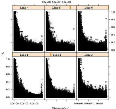
In theory, the linkage disequilibrium is higher in short distances and it decreases when the distance between markers increases. Nevertheless, a different behaviour was observed in chromosome 1 for all lines. Figure 1 shows high LD between distant SNP pairs in similar regions for all studied lines. Chromosomes 4, 5, 7, 9, 11, 12, 13, 14, 15 and 16 performed similarly, at a lesser intensity (Data Supplements). Figure 2 shows the LD behaviour in chromosome 2. There were differences in the LD decrease across the lines, the r² (LD measure) was particularly higher between distant SNPs in lines 1 and 6. Chromosome 3 (figure 3) has a linkage disequilibrium decrease comparable to the theory, the same was observed in chromosomes 6, 8 and 17 (Data Supplements).

Figure 1

(26)

16 Figure 2

Linkage Disequilibrium (r²) between SNP pairs in relation to physical distance between SNPs in pig chromosome 2 for six commercial lines.

Figure 3

Linkage Disequilibrium (r²) between SNP pairs in relation to physical distance between SNPs in pig chromosome 3 for six commercial lines.

(27)

17 rapidly. It can be observed that all lines presented similar average r² in the different distances.

Figure 4

Average r2 across lines at different marker distance for all chromosomes

Haplotype block structure

(28)

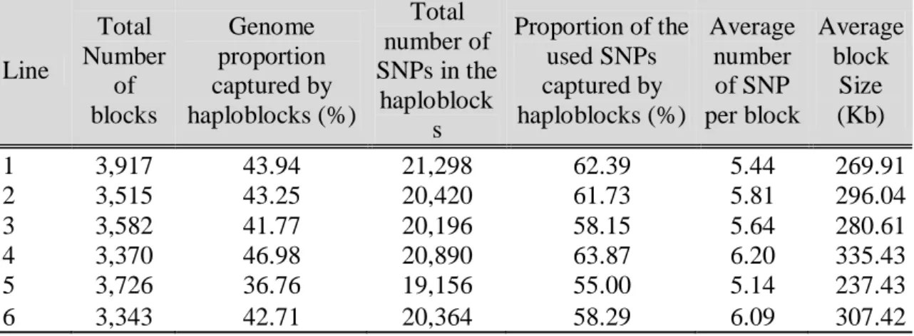
18 proportion of the genome captured by haplotype blocks ranged from 46.98 % on line 4 to 36.76 % on line 5. Line 1 had the highest number of SNPs captured by blocks (21,298), but line 4 had the highest proportion (63.87%) of captured SNPs in relation to the SNPs used. Line 5 had the lowest number (19,156) and proportion (55.00%) of captured SNPs. This descriptive analysis by each autossome was done and is exhibited in Data Supplements.

In general, the number of blocks differed between lines and chromosome, only the SSC9 the lines 3 and 5 had the same number of blocks (265) but they differed in the number of SNPs in the blocks and average block size. The same occurred with lines 2 and 4 and 5 and 6 on autossome 10 and on autossome 16 with lines 3 and 4. Smaller or higher block size did not predominate in a specific line, the average block size depended on the line and chromosome. Generally, all lines and chromosomes had a higher standard deviation regarding block size (Data Supplements).

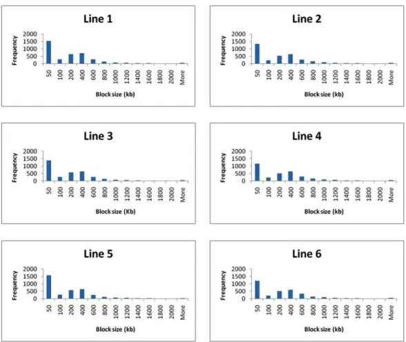
Figure 5 illustrates the block size frequency considering all autosomes. The six lines show a higher frequency of blocks with less than 50 Kb and blocks with more than 800 Kb occur at low frequency in all lines.

Table 2: Total number of blocks, genome proportion captured by haplotype blocks, total number of SNPs in the haplotype blocks, proportion of the used SNPs captured by haplotype blocks, average number of SNPs per block and average block size.

Line Total Number of blocks Genome proportion captured by haploblocks (%) Total number of SNPs in the

haploblock s

Proportion of the used SNPs captured by haploblocks (%) Average number of SNP per block Average block Size (Kb)

1 3,917 43.94 21,298 62.39 5.44 269.91

2 3,515 43.25 20,420 61.73 5.81 296.04

3 3,582 41.77 20,196 58.15 5.64 280.61

4 3,370 46.98 20,890 63.87 6.20 335.43

5 3,726 36.76 19,156 55.00 5.14 237.43

6 3,343 42.71 20,364 58.29 6.09 307.42

(29)

19 Figure 5

Block Size frequency in six pig lines considering all autossomes.

(30)

20 *Significant comparison (p-value<0.05)

Figure 6

Contrasts between pig lines considering all autossomes evaluated using the t-test.

(31)

21 Table 3: Contrast estimate, standard error and P-value of the significant line comparisons by autossome.

Autossome Contrast

Contrast Estimate

Standard

Error P-value

1 3 vs 5 45.731 25.028 0.068

1 3 vs 6 41.908 25.077 0.095

2 4 x 6 61.174 31.539 0.053

3 1 vs 5 33.650 20.178 0.096

3 3 vs 5 36.148 20.413 0.077

5 1 vs 4 -49.159 25.067 0.050

5 2 vs 4 -46.215 24.876 0.063

5 4 vs 6 47.498 25.617 0.064

7 3 vs 4 -45.122 22.748 0.048

7 4 vs 6 37.591 22.666 0.097

9 1 vs 3 37.622 18.857 0.046

9 1 vs 5 39.640 18.861 0.036

9 3 vs 6 -35.140 19.931 0.078

9 5 vs 6 -37.158 19.966 0.063

10 4 vs 5 45.977 23.889 0.055

15 1 vs4 -79.789 41.770 0.056

18 2 vs 3 44.580 19.738 0.024

18 3 vs 5 -49.339 19.895 0.013

18 3 vs 6 -33.225 19.477 0.089

18 Boar vs Sow 70.509 33.887 0.038

There were significant block size differences in autossomes 1, 2, 3, 5, 7, 9, 10, 15 and 18 (Table 3). Autossomes 9 and 18 had the largest number of significant comparisons, and in chromosome 18 the lines 2, 5 and 6 had greater block size than line 3, in addition the contrast in this chromosome between boar lines (1, 2 and 5) and sow lines (3, 4 and 6) was significant. A similar situation was observed in chromosome 5 where lines 1, 2 and 6 had smaller block sizes than line 4.

DISCUSSION

(32)

22 characterize the block. This report presents an LD analysis of six pig commercial lines covering all autossomes.

The number of genotyped animals diverges considerable among the lines, and line 1 had practically half of the genotyped animals (1008). It is well known that D’ is inflated with small sample sizes as demonstrated by Bohmanova et al. (2010), but the influence of this factor on the haplotype block estimation is reduced, since in the Gabriel et al. (2002) approach a narrow D’ confidence bound is used. In addition, the correlation of gene frequencies (r2) was used as linkage disequilibrium measurement to avoid the influence of small sample size and lower allele frequency, since it is considered a more robust linkage disequilibrium appraisal than D’ (Du, et al., 2007; Johnson, et al., 2001; Amaral, et al., 2008; Bohmanova, et al., 2010).

In theory, the concept of linkage disequilibrium is quite simple; it refers to the nonrandom segregation of markers that are closely linked. The expected behaviour is to observe a decrease in the LD with increase in distance, consequently high levels of linkage disequilibrium occur between SNPs in close proximity and a lower LD is expected for distant SNP pairs. However, a range of factors affect the recombination measurement such as genetic drift, demographic population history, selection and other factors which make the linkage disequilibrium highly variable even between closely linked markers (Ardlie, et al., 2002; Kruglyak, 1999; Pritchard and Przeworski, 2001).

Although a decrease in the LD with increase in distance was expected and observed in some chromosomes (3, 6, 8 and 17), high linkage disequilibrium was observed between SNPs at large distances for all lines in chromosomes 1, 4, 5, 7, 9, 10, 12, 13, 14, 15 and 16. It could be caused by the many factors that affect the LD as cited above. Nevertheless, the fact that high LD was observed in all the different lines studied leads us to suppose that it was caused by the accuracy of the genome assembly (Sscrofa10). Thus, the LD peaks observed in some chromosomes could be caused by mistakes in the order and distance between markers. The same problem was cited by Uimari and Tapio (2011), in a LD study using Sscrofa 9.

(33)

23 characteristic of each population, and in this case, the SSC 18 and SSC 2 showed a similar pattern for more than one line.

There are some important traits for the pig chain, that could be a selection objective for any line, that can make different pig lines present a similar LD behavior. In this way, the high linkage disequilibrium over markers at large distances could be explained by a selection effect. However, to confirm this hypothesis it would be necessary to identify which are the distant SNPs that are in linkage disequilibrium and to investigate the QTLs present at these regions.

In the current study marker pairs separated by 1500 – 3000 Kb had an average r2 of 0.12, which was similar to that reported by Du et al. (2007) for pigs that estimated an average r2 of 0.1 in a distance of 3 cM. In cattle, Qanbari et al. (2010) reported an average r2 of 0.3 between markers distant 25 kb and Bohmanova et al. (2010) found an average r2 of 0.2 between markers 40-60 Kb apart for North American Holstein cattle, both studies found lower r2 than that reported in the present study. Uimari and Tapio (2011) reported an average r² of 0.47 and 0.49 for Finnish Landrace and Finnish Yorkshire, respectively, for SNPs 30 Kb apart. In the present study, an average r² of 0.43, 0.47, 0.45, 0.47, 0.42 and 0.45 was observed for the lines 1, 2, 3, 4, 5 and 6, respectively for SNPs with less than 35 Kb apart.

An average r2 above 0.3 was found for all lines in markers between 105-175 Kb distance. This level of LD is suitable for association studies and genomic selection and considering that the pig genome size is 2.41 Gb (www.ensembl.org/sus_scrofa), it implies the use of 22,915 informative SNPs (MAF > 0.05) for whole genome studies.

The recommendation above is supported by Meuwissen et al. (2001) who reported in a simulation study that the required LD level for genomic selection was 0.2; Qanbari et al. (2010) considered that a threshold of 0.25 was a useful LD for association studies and Ardlie et al. (2002) defined an r2 > 1/3 as high values of LD. In pigs, Du et al. (2007) recommended marker spacing between 0.1 and 1 cM for whole association studies, in addition the authors considered an r2of 0.3 as a threshold of “usable” LD for association studies.

(34)

24 found that the blocks covered 4.7% of the bovine genome and included only 8% of all SNPs.

Although the average block size was 287.81 Kb, small blocks with less than 50 Kb predominated in the six evaluated pig lines. Amaral et al. (2008) analyzed three regions of the chromosomes 18 and 3 and observed that in Chinese pig breeds LD is mostly organized in blocks of up to 10 Kb and in European breeds the LD extents over haplotype blocks up to 400 kb. Although these results diverged from the current study, it is complex to compare the outcome from these studies, since in Amaral et al. (2008) the investigation was limited to three high density marked regions.

LD studies from humans and cattle can be used to make inferences about pigs, since it was reported that haplotype block structure is conserved across mammals (Guryev, et al., 2006). Qanbari et al. (2010) used 40,854 SNPs covering the whole bovine genome and observed 712 haplotype blocks with an average size of 164 Kb. Villa-Angulo et al. (2009) evaluated high density marker regions (on average one SNP per 4 Kb) of the bovine genome and reported haplotype blocks with an overall mean size of 10.3 Kb across 19 breeds, which according to the authors was similar to the block size observed in humans. An average block size of 7.3, 13.2, and 16.3 kb were observed in three human populations when ten 500 Kb regions with a density of approximately one SNP every 5 kb were analyzed (International HapMap Consortium, 2005).

It was expected that the average block size in pigs would be higher than in humans because of the natural aspects of livestock, such as small effective number, selection, crossing and genetic drift which contribute to increase the block size. The comparison with cattle studies is complicated because they have diverse outcomes, as showed above.

Some differences in SNP density between the lines were observed in this study, which can influence their haplotype block pattern. As a result, the block size was compared using the number of SNPs per block as covariate, in order to eliminate the influence of the marker density on the block size.

(35)

25 only an in-depth study of these haplotype blocks could give a better understanding of this divergence.

The significant differences between lines regarding block size are difficult to explain, because they could be caused by many factors. An investigation of the regions where the lines disagree regarding the haplotype blocks and their selection history might provide greater understanding of the significant differences and it would permit a solid explanation of this divergence.

CONCLUSIONS

According to the LD extent observed at this study, 22,915 informative SNPs (MAF > 0.05) would be necessary for whole genome association studies in the present lines. The high linkage disequilibrium observed in some chromosomes between distant SNPs may be caused by mistakes in the position and distance of the SNP marker. In addition, for some chromosomes (SSC2 and SSC18), the high LD may be caused by selection; but a in-depth study on the regions where these SNPs are found would be necessary to confirm this hypothesis. A concrete explanation for the divergences in haplotype block size can be made only with a more detailed study of the blocks.

LITERATURE CITED

Amaral A. J., H. J. Megens, R. P. M. A. Crooijmans, H. C. M. Heuven, M. A. M. Groenen. 2008. Linkage disequilibrium decay and haplotype block structure in the pig. Genetics. 179:569-579.

Ardlie K. G., L. Kruglyak, M. Seielstad. 2002. Patterns of linkage disequilibrium in the human genome. Nat. Rev. Genet. 3:299-309.

Barrett J. C., B. Fry, J. Maller, M. J. Daly. 2005. Haploview: analysis and visualization of LD and haplotype maps. Bioinformatics. 21:263-5

Bohmanova J., M. Sargolzaei, F.S. Schenkel. 2010. Characteristics of linkage disequilibrium in North American Holsteins. BMC genomics. 11:421.

Daly M. J., J. D. Rioux, S. F. Schaffner, T. J. Hudson, E. S. Lander 2001. High-resolution haplotype structure in the human genome. Nature genetics, 29:229-233. Du, F. X., A. C. Clutter and M. M. Lohuis. 2007. Characterizing linkage disequilibrium

(36)

26 Ensembl - www.ensembl.org/sus_scrofa.

Gabriel S. B., S. F. Schaffner, H. Nguyen, J. M. Moore, J. Roy, B. Blumenstiel, J. Higgins, M. DeFelice, A. Lochner, M. Faggart, S. N. Liu-Cordero, C. Rotimi, A. Adeyemo, R. Cooper, R. Ward, E. S. Lander, M. J. Daly, D. Altshuler. 2002. The structure of haplotype blocks in the human genome. Science. 296:2225-9.

Guryev V., B. M. G. Smits, J. V. D. Belt, M. Verheul, N. Hubner, E. Cuppen. 2006.

Haplotype Block Structure Is Conserved across Mammals. PLOS Genetics. 2:1111-1118.

Hill W. G and A. Robertson. 1968. Linkage disequilibrium in finite populations. Theoret. Appl. Genetics. 38:226-231.

International HapMap Consortium. 2005. A haplotype map of the human genome. Nature. 437:1299-1320.

Jeffreys A. J, L. Kauppi, R. Neumann. 2001. Intensely punctate meiotic recombination in the class II region of the major histocompatibility complex. Nature genetics. 29:217-222.

Johnson G. C. L., L. Esposito, B. J. Barratt, A.N. Smith, J. Heward, G. Di Genova, H. Ueda, H. J. Cordell, I. A. Eaves, F. Dudbridge, R. C. J. Twells, F. Payne, W. Hughes, S. Nutland, H. Stevens, P. Carr, E. Tuomilehto-Wolf, J. Tuomilehto, S. C. L. Gough, D. G. Clayton and J. A. Todd. 2001. Haplotype tagging for the identification of common disease genes. Nature genetics. 29:233-238.

Khatkar M. S., F. W. Nicholas, A. R. Collins, K. R. Zenger, J. Al Cavanagh, W. Barris, R. D. Schnabel, J. F. Taylor and H. W. Raadsma. 2008. Extent of genome-wide linkage disequilibrium in Australian Holstein-Friesian cattle based on a high-density SNP panel. BMC Genomics. 9:187.

Kruglyak L. 1999. Prospects for whole-genome linkage disequilibrium mapping of common disease genes. Nature genetics. 22:139-144.

Lewontin R. C. 1964. The Interaction of Selection and Linkage. I. General Considerations; Heterotic Models. Genetics, 49:49-67.

Meuwissen T. H. E., B. J. Hayes, M. E. Goddard. 2001. Prediction of Total Genetic Value Using Genome-Wide Dense Marker Maps. Genetics. 157:1819-1829.

Pig QTL database - www.animalgenome.org/cgi-bin/QTLdb/SS/index

(37)

27 Qanbari S, E. C. G. Pimentel, J. Tetens, G. Thaller, P. Lichtner, A.R. Sharifi, H. Simianer. 2010. The pattern of linkage disequilibrium in German Holstein cattle. Animal Genetics. 41:346-356.

Rothschild M. F., Z. Hu, Z. Jiang. 2007. Advances in QTL mapping in pigs Int. J. Biol. Sci. 3:192-7.

SAS Institute Inc., SAS 9.1.3 Help and Documentation, Cary, NC: SAS Institute Inc., 2000-2004.

The R Foundation for Statistical Computing. 2009. R version 2.10.1

Uimari, P. and M. Tapio. 2011. Extent of linkage disequilibrium and effective population size in Finnish Landrace and Finnish Yorkshire pig breeds. J. Anim. Sci. 89:609-614.

Villa-angulo R., L. K. Matukumalli, C. A. Gill, J. Choi, C. P. Van Tassell, J. J. Grefenstette.2009. High-resolution haplotype block structure in the cattle genome. BMC Genetics. 13:1-13.

(38)

28

DATA SUPPLEMENTS

Table 1. Number of SNPs in the beginning of analysis, the final number of SNPs used, average MAF and average distance between SNPs by chromosome

All Chromossomes Line

Initial number of SNPs

Final number of

SNPs Average MAF

1 41,785 34,138 0.279 70.481

2 41,785 33,081 0.286 72.733

3 41,785 34,438 0.289 69.283

4 41,785 32,706 0.278 73.567

5 41,785 34,828 0.291 69.085

6 41,785 34,937 0.285 68.869

SSC1 Line Initial number of

SNPs

Final number of

SNPs Average MAF

1 5,386 4,183 0.269 70.812

2 5,386 4,326 0.281 68.472

3 5,386 4,054 0.285 73.066

4 5,386 4,156 0.276 71.272

5 5,386 4,404 0.303 67.259

6 5,386 4,515 0.290 65.605

SNPs

Final number of

SNPs Average MAF

1 2,656 2,217 0.285 73.556

2 2,656 2,168 0.291 75.219

3 2,656 2,273 0.294 71.744

4 2,656 2,078 0.278 78.477

5 2,656 2,332 0.292 69.929

6 2,656 2,362 0.285 69.041

SNPs

Final number of

SNPs Average MAF

1 2,238 1,750 0.260 81.483

2 2,238 1,759 0.289 81.066

3 2,238 1,898 0.279 75.129

4 2,238 1,908 0.282 74.735

5 2,238 1,977 0.289 72.127

(39)

29 Cont. Table 1. Number of SNPs in the beginning of analysis, the final number of SNPs used, average MAF and average distance between SNPs by chromosome

SNPs

Final number of

SNPs Average MAF

1 2,964 2,552 0.279 54.274

2 2,964 2,211 0.285 62.644

3 2,964 2,435 0.290 56.881

4 2,964 2,292 0.277 60.430

5 2,964 2,456 0.305 56.395

6 2,964 2,300 0.283 60.220

SNPs

Final number of

SNPs Average MAF

1 1,915 1,546 0.270 71.502

2 1,915 1,590 0.291 69.524

3 1,915 1,463 0.286 75.559

4 1,915 1,453 0.261 76.079

5 1,915 1,623 0.293 68.110

6 1,915 1,565 0.278 70.634

SNPs

Final number of

SNPs Average MAF

1 2,411 2,050 0.294 76.834

2 2,411 1,953 0.293 80.650

3 2,411 2,070 0.293 76.092

4 2,411 1,913 0.257 82.337

5 2,411 1,989 0.285 79.191

6 2,411 2,038 0.295 77.287

SNPs

Final number of

SNPs Average MAF

1 2,780 2,125 0.271 63.097

2 2,780 2,203 0.287 60.863

3 2,780 2,152 0.296 62.306

4 2,780 2,070 0.271 64.774

5 2,780 2,288 0.281 58.602

(40)

SNPs

Final number of

SNPs Average MAF

1 2,177 1,825 0.284 80.919

2 2,177 1,652 0.288 89.393

3 2,177 1,887 0.294 78.260

4 2,177 1,634 0.272 90.377

5 2,177 1,439 0.272 102.624

6 2,177 1,834 0.288 80.522

SNPs

Final number of

SNPs Average MAF

1 2,578 2,074 0.284 73.322

2 2,578 2,120 0.278 71.731

3 2,578 2,264 0.284 67.169

4 2,578 2,128 0.276 71.461

5 2,578 2,279 0.302 66.727

6 2,578 2,153 0.263 70.632

SNPs

Final number of

SNPs Average MAF

1 1,299 1,100 0.278 73.278

2 1,299 1,054 0.284 76.476

3 1,299 1,084 0.287 74.360

4 1,299 1,065 0.278 75.687

5 1,299 1,137 0.291 70.894

6 1,299 1,151 0.284 70.031

SNPs

Final number of

SNPs Average MAF

1 1,561 1,328 0.293 63.386

2 1,561 1,226 0.286 68.660

3 1,561 1,265 0.262 66.543

4 1,561 1,163 0.283 72.379

5 1,561 1,328 0.287 63.386

(41)

SNPs

Final number of

SNPs Average MAF

1 1,247 1,009 0.284 63.707

2 1,247 1,024 0.294 62.773

3 1,247 1,089 0.292 59.027

4 1,247 1,071 0.277 60.019

5 1,247 1,138 0.301 56.485

6 1,247 1,074 0.307 59.851

SNPs

Final number of

SNPs Average MAF

1 2,966 2,315 0.279 91.962

2 2,966 2,355 0.285 90.400

3 2,966 2,416 0.285 88.118

4 2,966 2,258 0.298 94.284

5 2,966 2,526 0.298 84.280

6 2,966 2,470 0.284 86.191

SNPs

Final number of

SNPs Average MAF

1 3,292 2,785 0.279 55.180

2 3,292 2,661 0.290 57.752

3 3,292 2,896 0.315 53.065

4 3,292 2,653 0.300 57.926

5 3,292 2,804 0.284 54.806

6 3,292 2,685 0.291 57.235

SNPs

Final number of

SNPs Average MAF

1 2,270 1,945 0.286 78.535

2 2,270 1,726 0.282 88.499

3 2,270 1,810 0.271 84.392

4 2,270 1,689 0.273 90.438

5 2,270 1,805 0.266 84.626

(42)

SNPs

Final number of

SNPs Average MAF

1 1,554 1,320 0.285 65.149

2 1,554 1,198 0.298 71.783

3 1,554 1,263 0.293 55.374

4 1,554 1,227 0.281 70.087

5 1,554 1,332 0.296 64.562

6 1,554 1,249 0.294 68.852

SNPs

Final number of

SNPs Average MAF

1 1,399 1,108 0.271 62.646

2 1,399 1,083 0.274 64.092

3 1,399 1,183 0.277 58.675

4 1,399 1,089 0.278 63.739

5 1,399 1,190 0.291 58.329

6 1,399 1,165 0.297 59.581

SNPs

Final number of

SNPs Average MAF

1 1,092 906 0.294 66.248

2 1,092 772 0.260 77.747

3 1,092 936 0.299 64.125

4 1,092 859 0.269 69.873

5 1,092 781 0.259 76.851

6 1,092 878 0.268 68.361

(43)

33 Figure 1

Linkage Disequilibrium between SNP pairs in relation to physical distance between loci in pig chromosome 1 for six commercial lines.

Figure 2

(44)

34 Figure 3

Figure 4

(45)

35 Figure 5

Figure 6

(46)

36 Figure 7

Figure 8

(47)

37 Figure 9

Figure 10

(48)

38 Figure 11

Figure 12

(49)

39 Figure 13

Figure 14

(50)

40 Figure 15

Figure 16

(51)

41 Figure 17

Figure 18

(52)

42 Table 2. Number of blocks, total number of SNPs in the blocks, average number SNP / block, standard deviation number of SNP / block, average block size (Kb), standard deviation block size (Kb), maximum block size (Kb) and minimum block size (Kb).

SSC1 Line

Number of blocks

Total number of SNPs in the

blocks Average number of SNP/ block SD number of SNP/ block Average block size (Kb) SD block size (Kb) Maximum Block size (Kb) Minimum block size (Kb)

1 415 3,018 7.272 7.513 407.711 649.653 0.028 5658.450

2 410 3,049 7.437 6.539 398.807 533.019 0.028 3810.670

3 382 2,939 7.694 8.150 454.669 892.514 0.358 9889.490

4 391 2,850 7.289 6.611 393.074 531.058 0.025 3973.860

5 420 2,956 7.038 6.447 360.708 520.886 0.025 4484.410

6 416 3,187 7.661 7.116 410.359 589.244 0.025 5303.950

SSC2 Line

Number of blocks

1 273 1,484 5.436 4.310 257.003 404.701 0.120 3176.680

2 243 1,398 5.753 5.182 309.329 637.668 0.153 6314.630

3 271 1,328 4.900 3.797 236.270 433.180 0.153 4878.920

4 221 1,451 6.566 7.264 384.586 707.005 0.153 4790.340

5 293 1,353 4.618 3.755 201.700 398.609 0.153 4069.410

(53)

43 Cont. Table 2. Number of blocks, total number of SNPs in the blocks, average number SNP / block, standard deviation number of SNP / block, average block size (Kb), standard deviation block size (Kb), maximum block size (Kb) and minimum block size (Kb).

SSC3 Line

Number of blocks

1 224 1,024 4.571 3.555 222.899 348.721 0.165 2309.850

2 199 1,066 5.357 4.303 280.085 436.220 0.078 3633.280

3 216 1,084 5.019 3.967 257.602 406.892 0.078 3673.590

4 227 1,070 4.714 3.673 212.348 303.108 0.761 1741.430

5 243 987 4.062 2.840 152.532 227.254 0.165 1416.070

6 206 992 4.816 3.986 216.364 330.359 0.078 1891.680

SSC4 Line

Number of blocks

1 310 1,554 5.013 4.991 196.349 435.027 0.180 6656.220

2 236 1,297 5.496 5.630 235.413 474.297 0.651 5255.580

3 240 1,415 5.896 6.720 248.801 457.508 0.651 5431.330

4 243 1,463 6.021 6.156 274.070 510.712 1.310 6211.920

5 247 1,338 5.417 5.850 208.934 443.406 0.651 5341.820

(54)

SSC5 Line

Number of blocks

1 166 851 5.127 4.036 240.734 386.136 3.246 2835.580

2 171 904 5.287 4.728 256.248 467.214 1.076 4447.230

3 159 763 4.799 3.598 226.575 294.402 0.017 1745.980

4 162 918 5.667 4.772 332.321 498.366 0.017 4028.970

5 177 780 4.407 3.121 198.564 313.192 0.186 1945.660

6 152 820 5.395 4.288 263.464 370.645 0.017 1825.990

SSC6 Line

Number of blocks

1 256 1,423 5.559 5.803 303.521 657.056 0.161 6075.710

2 238 1,251 5.256 4.854 272.235 543.398 0.164 5482.680

3 246 1,367 5.557 5.459 299.627 579.075 0.061 5647.650

4 221 1,299 5.878 5.242 335.502 569.661 0.164 5098.040

5 228 1,198 5.254 4.899 265.950 497.240 0.061 3601.010

(55)

SSC7 Line

Number of blocks

1 206 1,196 5.806 4.857 266.944 380.293 0.189 2594.350

2 214 1,303 6.089 6.417 269.331 446.712 2.003 3889.550

3 193 1,087 5.632 5.740 225.973 371.153 2.798 2536.370

4 204 1,167 5.721 5.385 276.376 442.455 2.003 2860.270

5 216 1,227 5.681 5.530 241.824 385.482 2.003 3676.670

6 196 1,226 6.255 6.774 270.695 451.560 2.003 4286.290

SSC8 Line

Number of blocks

1 211 1,163 5.512 5.891 342.879 633.601 0.317 4885.830

2 182 1,060 5.824 6.035 371.049 903.434 0.250 9654.750

3 217 1,009 4.650 3.402 249.708 444.328 0.301 3255.010

4 158 1,024 6.481 7.104 490.930 1439.820 0.314 16589.580

5 168 800 4.762 4.397 292.754 454.570 0.250 2463.200

(56)

SSC9 Line

Number of blocks

1 277 1,302 4.700 4.016 239.480 413.730 0.069 3480.660

2 251 1,352 5.386 4.499 257.768 370.103 0.360 2272.700

3 265 1,266 4.777 4.361 207.247 333.159 0.030 2552.340

4 246 1,386 5.634 5.070 282.608 417.853 0.069 2378.920

5 265 1,164 4.392 4.097 178.290 308.094 0.153 2016.850

6 225 1,295 5.756 4.946 310.849 449.450 0.153 2376.340

SSC10 Line

Number of blocks

blocks Average number of SNP/ block Sd number of SNP/ block Average block size (Kb)

Sd block size (Kb)

Maximum Block size

(Kb)

Minimum block size (Kb)

1 126 500 3.968 3.392 155.350 292.867 0.035 1988.280

2 113 452 4.000 2.712 147.799 229.374 2.083 1424.600

3 109 487 4.468 2.911 183.127 259.740 0.077 1375.860

4 113 610 5.398 4.918 280.150 469.651 0.077 3567.660

5 115 460 4.000 2.421 134.943 211.903 1.159 1491.330

(57)

SSC11 Line

Number of blocks

1 153 704 4.601 3.767 192.548 299.038 0.170 2063.090

2 130 636 4.892 5.257 232.806 529.103 0.170 4411.690

3 131 672 5.130 7.344 250.897 633.445 0.170 6382.570

4 133 677 5.090 7.817 254.693 664.822 1.666 6691.500

5 148 643 4.345 4.191 177.213 387.809 0.170 3189.320

6 114 659 5.781 8.315 275.943 688.055 0.170 6745.410

SSC12 Line

Number of blocks

Sd block size (Kb)

Maximum Block size

(Kb)

1 148 567 3.831 3.157 121.874 229.591 0.029 1968.790

2 130 532 4.092 3.214 147.389 230.071 0.029 1110.500

3 145 534 3.683 2.715 109.896 187.949 0.029 1110.010

4 137 594 4.336 3.088 153.116 240.316 0.029 1574.380

5 145 567 3.910 3.356 123.964 227.085 0.029 1574.380

(58)

48 Cont. Table 2. Number of blocks, total number of SNPS in the blocks, average number SNP / block, standard deviation number of SNP / block, average block size (Kb), standard deviation block size (Kb), maximum block size (Kb) and minimum block size (Kb).

SSC13 Line

Number of blocks

1 269 1,637 6.086 5.254 414.672 751.277 1.412 6663.270

2 231 1,606 6.952 8.179 442.527 827.449 0.362 7971.370

3 234 1,540 6.581 8.014 437.107 838.698 0.362 7452.140

4 215 1,559 7.251 9.560 512.289 931.154 0.385 7197.040

5 280 1,594 5.693 4.964 359.720 582.458 0.162 5046.620

6 200 1,682 8.410 9.624 575.979 959.058 0.385 5919.680

SSC14 Line

Number of blocks

Sd block size (Kb)

Maximum Block size