Bandwidth usage distribution of multimedia servers using Patching

(1)

Bandwidth usage distribution of multimedia

servers using Patching

q

Carlo K. da S. Rodrigues

*

_{, Rosa M.M. Lea˜o}

Federal University of Rio de Janeiro, COPPE/PESC, CxP 68511, Rio de Janeiro RJ 21941-972, Brazil Received 28 June 2005; received in revised form 5 March 2006; accepted 12 May 2006

Available online 13 June 2006

Responsible Editor: J. Misic

Abstract

Several multicast bandwidth sharing techniques have been proposed in the literature to provide more scalability to multimedia servers. These techniques are often analyzed in terms of the average bandwidth requirements they demand to satisfy client requests. However, average values do not always provide an accurate estimate of the required bandwidth. Therefore, they cannot be the only parameter used to guarantee a certain level of quality to the clients. In this work we propose a simple analytical model to accurately calculate the distribution of the number of concurrent streams or, equiv-alently, the bandwidth usage distribution considering the popular Patching technique. We show that the distribution may be modeled as a binomial random variable in the single object case, and as a sum of independent binomial random vari-ables in the multiple object case. Through simulation we validate our results. Moreover, we also illustrate how these results may be practically used for instance (i) to allocate bandwidth to provide a given level of QoS, (ii) to estimate the impact on QoS when some system parameters dynamically change, and (iii) to conﬁgure the overall system.

Keywords: Patching; Multicast; Multimedia; Bandwidth; QoS

1. Introduction

Multimedia servers for applications such as dis-tance learning and video on demand have been the

focus of recent studies in the literature. In particu-lar, considerable attention has been given to the issue of providing scalability to these servers. The easiest way to service client requests in such applica-tions is to schedule unicast data streams, one for each client request. The multimedia server band-width increases linearly with the client arrival rate since clients arrive and presumably stay in the system for some reasonable time (i.e., it increases linearly with the number of concurrent clients in the system). This increase rate notably precludes

doi:10.1016/j.comnet.2006.05.004

q

This work is supported in part by grants from CNPq and Faperj.

*

Corresponding author. Tel.: +55 21 2562 8664; fax: +55 21 2562 8676.

E-mail addresses:kleber@land.ufrj.br(C.K.d.S. Rodrigues), rosam@land.ufrj.br(R.M.M. Lea˜o).

(2)

the use of this service for a very large number of cli-ents and the study of bandwidth sharing techniques becomes essential to provide scalability.

Bandwidth sharing techniques may be classiﬁed in multicast or periodic broadcast delivery tech-niques. Multicast techniques (e.g., [1–3,5–10,12]) are reactive in the sense that data is delivered in response to client requests. Most of them provide immediate service and save server bandwidth by avoiding unnecessary transmission of data. Periodic broadcast delivery techniques (e.g., [13–21]) cycli-cally transmit object segments in a proactive way. They can guarantee a maximum start up delay. The idea is to divide the media object into a series of segments and broadcast each segment periodi-cally on dedicated server channels. While the client is playing the current object segment, it is guaran-teed that the next segment is downloaded on time and the whole object can be played out continu-ously. Besides multicast and periodic broadcast, an orthogonal scheme for reducing the load on net-work and video server is video caching (see [44]

and references within). In this scheme a set of prox-ies are strategically placed close to the clients. Another approach to address the scalability issue in video applications is peer-to-peer streaming (see

[46]and references within). In this approach clients can serve other clients by forwarding the video stream.

Patching[2]is a multicast technique and has been used in recent works[22,45,23–28]. For example, in

[22]Patching is used to provide a peer-to-peer video streaming service, and in [45] it is integrated with proxy caching for media distribution. This technique is especially attractive because of its extreme simplic-ity and competitive eﬃciency in terms of bandwidth savings. The work of[29]for instance evaluated the complexity of several multicast delivery techniques. The analysis is based on the information the server has to keep and theworkthe server has to perform per client request. One of the main results they obtained is that Patching is one of the simplest schemes. And it was shown in the work of[7,9]that, for reasonably popular media objects, the average bandwidth requirements of Patching are very similar to those of much more complex techniques.

It is quite common to evaluate the eﬃciency of multicast techniques in terms of the average band-width requirements they demand to satisfy the client requests arriving in the system. A discussion about average bandwidth requirements may be found in

[5–7,30–33]. However, average values do not always

provide an accurate estimate of bandwidth require-ments and therefore cannot be used solely to guaran-tee a given level of QoS to the clients. Tam and co-workers[29]were the ﬁrst to measure the perfor-mance of multicast techniques using other metrics such as the maximum bandwidth and the bandwidth distribution. The authors have focused on three merge techniques: the dynamic Fibonacci tree

[9,34], the Dyadic [10], and the earliest reachable merge target (ERMT) [7]. Their analysis was all based on simulations.

The quality of service of multicast techniques was also evaluated in[28,33]. De Souza e Silva et al.[28]

proposed an algorithm to compute the distribution of the bandwidth required by the Patching tech-nique. Their analytical model estimates the distribu-tion of the total requested bandwidth in one window of Patching. They showed that the requested data streams in a window are a good estimator of the data streams actually transmitted in a window as

t_{! 1}. The computational cost of their algorithm is O(P2), wherePis a function of the estimated error and is usually not very large. Their results indicated that if the server conﬁguration is based on the aver-age bandwidth required by each object, the proba-bility of requiring more than the average value is large for a wide range of system parameters.

In[33]approximate analytical models were deve-loped to analyze the quality of service of the following schemes: Patching, Hierarchical Stream Merging (HSM) [7]and Bandwidth Skimming [8]. The authors used a closed queueing network model to estimate two performance measures: the mean client waiting time and the fraction of clients who leave without receiving service when the server is temporarily overloaded (i.e., the balking rate). The performance measures were computed from the iterative solution of a set of equations. Their results showed for instance that if server conﬁguration is based on the average bandwidth there may be unac-ceptably high client balking rates.

We may see that the analytical evaluation of the Patching mechanism done so far is based on the solution of one equation [28] or a set of equations

[33], i.e., there is not a closed-form solution for the bandwidth usage distribution that may be prac-tically employed. Moreover, in [28] they only consider the single object case, and in[33]they only analyze the multiple object case.

(3)

the bandwidth usage distribution for the Patching technique. We consider both the single and the mul-tiple object cases. We show that the distribution may be modeled in the form of a closed-form solu-tion as a binomial random variable in the single object case. In the multiple object case, it can be represented as a sum of independent binomial random variables, which may be easily implemented using Fast Fourier Transform[38]. Through simula-tion we validate our results. Moreover, we illustrate how our results may be practically used to (i) allo-cate bandwidth to provide a given level of QoS, (ii) estimate the impact on QoS when some system parameters dynamically change, and (iii) conﬁgure the overall system.

The remainder of this paper is organized as fol-lows. Section 2 introduces some basic concepts and terminology. Section 3is dedicated to the pre-sentation of our analytical model. Analytical and simulation results are presented in Section4. Lastly, conclusions and ongoing work are included in Section5.

2. Basic concepts and terminology

Consider a multimedia server and a group of cli-ents receiving object streams (e.g., a ﬁlm, a video clip, etc.) across the Internet from this server. The paths from the server to the clients are multicast enabled. Multicast is not currently deployed over the global Internet. However, this can be alleviated through the use of proxies which can bridge unicast and multicast networks. One of the most common proposed architectures consists of a unicast channel from the server to the proxy and multicast channels from the proxy to the clients. Since, in general, the proxy and the clients are in the same local area net-work, multicast service can be easily implemented. Solutions like application level multicast using tun-nelling have also been used over the public Internet

[29,42,43].

Still assume that Patching is used to provide immediate service, clients always request playback from the beginning of the object and watch it con-tinuously till the end without any interruptions (i.e., sequential access), and client bandwidth is twice the object play rate. All these assumptions are considered in the original model of Patching presented in[2]. Also, consider that the client buﬀer is large enough to store a portion of the object size (to allow the stream synchronization). This supposi-tion is based on the results presented in the works of

[30,4,5]. These works show that, since the client bandwidth is twice the object play rate, in the worst case, the client will listen to two concurrent streams during an interval equal to half of the object size. However, since it is possible to compute an optimal threshold window [30,31], we may relax this initial supposition for the client buﬀer being half of the object size and set it to the optimal threshold win-dow. Lastly, Table 1 summarizes some notation used in the rest of this work.

The Patching technique operates as follows [2]. The server begins to deliver a full-object multicast stream upon the arrival of the ﬁrst client. The following clients who request the same object and arrive within a certain time interval, denoted as threshold window, retrieve the stream from the multicast channel (buﬀering the data) and obtain the missing initial portion, denoted as patch, directly from the server over a unicast channel; for clients arriving after the threshold window, a new session is initiated and the process restarts again. Both the multicast and patch streams deliver data at the object play rate so that each client can play the object in real time.

Similar models have been proposed in[30,31]to estimate the average server bandwidth for the Patching technique. They assumed a Poisson client arrival process with rate k_j for the media object

Oj, where j= 1,. . .,u and u is the total number of

objects in the server. The average server bandwidth for delivering objectOjis[30,31]:

Bj¼

Djþ

k_jW2_j

2 Wjþk1_j

; ð1Þ

where Dj and Wj are the length and the threshold

window, respectively, for objectOj.

Table 1 Key parameters

k_j _{Client arrival rate for object}Oj Dj Total length of objectOjin units of time Wj Threshold window for objectOjin units of time Nj Average number of requests for objectOjthat arrive

during the period of lengthDj. It is referred as object popularity and is given byNj=kjDj

Bj Average server bandwidth used to deliver objectOjusing the Patching technique in units of the object play rate dj Unit length used for objectOj

(4)

The denominator of Eq.(1) is the average time that elapses between successive full-object multi-casts, i.e., the duration of the threshold window plus the average time until the next client request arrives. The numerator is the expected value of the sum of the transmission times of the full-object and the patch streams that are initiated during the interval. Note that the average number of patches that are started before the threshold window expires isk_j_W_j_,

and the average duration of a patch isWj/2[35].

Now diﬀerentiating Eq. (1) with respect to Wj

and setting the result to zero gives

Wj;optimal¼

ffiffiffiffiffiffiffiffiffiffiffiffiffiffiffiffi

2Njþ1

p

1

k_j : ð2Þ

As already mentioned, the client buﬀer can be equal to the optimal threshold windowWj,optimal, instead

of half of the object size. Substituting (2) into Eq. (1) yields the following result for the average server bandwidth for the optimized Patching technique:

Bj;optimized¼

2Njþ1

p

1; ð3Þ

where Nj=kjDj is the average number of client

requests that arrive during Dj. The parameter Nj is

often denoted as the object popularity. For simplic-ity, we will refer to the optimized Patching technique as the Patching technique, and we will denote

Wj,optimalandBj,optimizedasWjandBj, respectively.

When the object popularityNjis above (below) a

certain threshold value, periodic broadcast delivery techniques achieve more (less) bandwidth savings than multicast ones [14]. Thus, it is reasonably to classify media objects in accordance with popularity in order to choose the most adequate type of delivery technique[30,14]. This is usually done as follows[8]: forhotobjects (i.e., NjP100), use periodic

broad-cast techniques; for cold objects (i.e., Nj< 10) and lukewarmobjects (i.e., 106Nj< 100), use multicast

techniques. Since Patching is a multicast technique, we mainly focus onNjvalues in the range of 10–100.

3. Bandwidth usage distribution

In this section, we present our analytical model and derive the distribution of the number of concur-rent streams needed by the Patching technique, or equivalently, the server bandwidth usage distribu-tion. We initially address the case of the single object and then the case of multiple objects.

3.1. Single object

Consider a server implementing the Patching technique and that client request arrivals follow a Poisson process. Let C(t) be the stochastic process which denotes the number of Patching windows opened in the interval (0,t). It thus directly follows that C(t) is a renewal process [35] whose renewal points correspond to the instants at which the server schedules a new full-object multicast stream, i.e., the start of a new window. Moreover, we have that a cycle of C(t) has an average duration of Wj+

1/k_j₌_W_j₊_D_j_/_N_j_{, and then this is the base interval}

we consider in the analysis to follow.

Now assume that the object Oj is divided into

time units of length dj. For example, a two-hour

object can be divided into 20 units of 6 min each, or divided into 100 units of 72 s each. Now let

Tj=Dj/dj and wj=Wj/dj. Then, we have that Tj

andwjare, respectively, the object size and the

win-dow size measured in number of discrete units of lengthdj. Also consider that if there is at least one

client arrival in a time unit, the server initiates a stream (patch or full-object multicast) at the begin-ning of the next time unit to serve this client. We stress that the value ofdjcan be as small as desired

to obtain a very small probability of more than one arrival in the same time unit and a guarantee of immediate service.

Note that since the media object and time in our model are divided into units of length dj, the base

interval of our analysis Wj+Dj/Nj may

alterna-tively be rewritten as wj+Tj/Njand Eq. (2)as

wj¼

Tj

2Njþ1

p

1

Nj

: ð4Þ

The interval wj+Tj/Nj is composed by a total of wj+Tj/Nj units of length dj. Hence, this interval

can still be expressed in the following form: [1,wj+Tj/Nj]. Let us now focus on each one of its wj+Tj/Nj units individually in order to identify a

distribution for the number of concurrent streams in each one of them. Once we obtain these individ-ual distributions, we try to identify a unique distri-bution that may be deployed for the entire base interval of analysis [1,wj+Tj/Nj].

Note thatOjmay be any object in the multimedia

server, then we drop the subscript j from now on. Consider thekth interval [1,w+T/N] of the process

(5)

patches. Then, we have that the number of concur-rent streams in each unit of lengthdof thekth inter-val is given by a multicast component plus a patch component.

Let us denote the multicast component as MC.

We consider MC as a constant value and estimate

it using Little’s result [36]: MC¼N=

ffiffiffiffiffiffiffiffiffiffiffiffiffiffiffi

2Nþ1 p

(i.e., the average number of multicast streams is given by the arrival rate times the duration of the media object). Although the real number of multicast streams is not constant due to the possible variation of the arrival ratek_{(and consequently of}_N_),_M_C_is

a good approximation since changes on the arrival ratek_{, within certain limits, do not severely impact}

on the value of MC. Consider N1, which refers

to the scenarios we are interested in. In this case

MC can be approximated by MC¼N=

ffiffiffiffiffiffiffi

2N

p ¼ 0:707 ffiffiffiffi

N

p

. Thus we have that the number of multi-cast streams increases approximately with the square root of the arrival rate.

The patch component is associated to client arrivals and we estimate it as a random variable. Our goal now is to determine the distribution of this random variable. Let us examine two successive intervals: the (k1)th and kth intervals. We want to determine how many units of the kth interval can transmit a patch initiated in the (k1)th inter-val. Note that we only need to consider the (k1)th interval because the patches generated in other pre-vious intervals will ﬁnish before the kth interval starts. Consider that thekth interval is divided into two sub-intervals: [1,wT/N] and [wT/N+ 1,

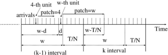
w+T/N]. In the former we may have transmissions initiated in the (k1)th interval, while in the latter we do not have any transmission initiated in the pre-vious interval. Fig. 1 shows a scenario where an arrival occurs in the last unit of the (k1)th inter-val. This arrival generates the longest possible patch which is equal to w. We note that the number of units in the kth interval, transmitting a patch stream initiated in the (k1)th interval, decreases as the value of T/N increases. In the limit, when

T/N=w(see Eq. (4)), all patches are initiated and transmitted in the same interval. Note that we do not need to consider scenarios where T/N>w

because this condition occurs only for N= 1 (see Eq. (4)). Bandwidth sharing techniques are mostly useful when N> 1. We mainly focus on the values ofNin the range of 10–100, as already mentioned. We proceed in three steps to obtain the distribu-tion of the number of concurrent patch streams in each unit of thekth interval. We ﬁrst compute the number of concurrent streams in the ith unit of the (k1)th andkth intervals assuming that there is a client arrival in each unit of the window wof the (k1)th interval. In the second step we com-pute the number of concurrent streams in the ith unit of the kth interval considering that there is a client arrival in each unit of both windows w of the (k1)th and kth intervals. Finally, in the third step, we analyze the impact of the Poisson client request arrival process.

Let us consider the ﬁrst step. As just mentioned, we only observe the patches started in the (k1)th interval and assume that there is a client arrival in each unit of the window w of this interval. Fig. 1

shows that an arrival in thejth unit of the interval generates a patch of lengthj units. Then, there is a patch in the ith unit of the (k1)th interval if, and only if, 2jPi, j= 1, 2,. . .,i1, and a client

arrival occurs in thejth unit. We can also see from

Fig. 1 that the longest possible patch initiated in the (k1)th interval starts at w+ 1 and ends at 2w. Therefore the interval we have to evaluate is [1, 2w]. We denote bymi,wthe number of concurrent

streams in theith unit of the interval [1, 2w], where

i= 1, 2,. . ., 2w. The following lemma determines

an expression formi,w.

Lemma 1. Considering one client arrival in each unit of the interval [1, w] and i = 1, 2,. . ., 2w, the number of concurrent patch streams mi,win the ith unit of the

interval [1, 2w] is given by

• _{Case 1: i}₂_{[1, w].}

mi;w¼

X

i1

j¼1

1f2jPig ¼ i₂1

: ð5Þ

• _{Case 2: i}₂_{[w + 1, 2w].}

mi;w¼

Xw

j¼1

1f2jPig ¼ 2w ð₂i1Þ

; ð6Þ

where 1 denotes the indicator function, i.e.,

1{x}= 1 if x is true, and1{x}= 0 if x is false.

d

w w

w-T/N

T/N T/N

Time patch=w

w-d arrivals

(k-1) interval k interval 4-th unit

patch=4 w-th unit

(6)

Proof. SeeAppendix A. _h

So far we obtained expressions to calculatemi,w,

i.e., the number of concurrent streams in the (k1)th and kth intervals considering the patches exclusively initiated in the (k1)th interval. We now present the second step of our analysis. Let

li,wbe the number of concurrent streams in thekth

interval [1,w+T/N], considering the patches initi-ated in this interval as well as in the previous one. We show that li,w can be easily computed by

properly superposing the expressions obtained in

Lemma 1.

Fig. 2illustrates the superposition of two succes-sive intervals: the (k1)th andkth intervals. From this ﬁgure we can see that the number of concurrent patches in the ﬁrst unit of thekth interval is equal to

m1,w+mw+T/N+1,w, in the second unit it is equal to m2,w+mw+T/N+2,w, and so on. The ﬁnal

formula-tion forli,w is presented inLemma 2.

Lemma 2. Considering one client arrival in each unit

of both windows w of the (k1)th and kth intervals

and i = 1, 2,. . ., w + T/N, the number of concurrent streams li,win the ith unit of the kth interval is given

by

• _{Case 1:}_i₂ ₁_;_wT

N

li;w ¼ wT

N

2 þ1; if ðw

T

NÞand i are even; wT

N 2

l m

; otherwise:

8 <

:

ð7_Þ

• _{Case 2:}_i₂ _wT

Nþ1;w

li;w¼

i1

2

: ð8_Þ

• _{Case 3:}_i₂ _w_þ₁_;_w_þT

N

li;w ¼

2w ði1Þ 2

: ð9Þ

Proof. SeeAppendix B. _h

We now proceed to the third step. Assume that client arrivals are represented by a Poisson process. Let Xibe a random variable that denotes the

num-ber of concurrent streams due to patches in the ith unit of the interval [1,w+T/N], where i= 1,. . ., w+T/N. Consider the scenario of Fig. 3 and let us examine the possible values taken, for example, by X4. To simplify the ﬁgure we do not represent

patches eventually generated in the previous inter-val. X4 may be equal to 0, 1 or 2, depending on

the client arrivals in the previous units.X4= 1 when

there is one arrival in the second or in the third unit (seeFig. 3(a) and (b), respectively). InFig. 3(c) we have the case where X4= 2, i.e., when there is an

arrival in both the second and third units. Lastly,

X4= 0 when there are arrivals neither in the second

nor in the third units. Note that we do not need to make assumptions about the ﬁrst unit because only the second and third units of this interval generate patches long enough to extend over the fourth unit. The following theorem determines the probabil-ity distribution function of Xi.

Theorem 1. Xihas binomial distribution with

param-eters p = 1eN/T and ni,w, i = 1,. . ., w + T/N. The parameter ni,wis given by

1. Case 1:w¼T

N, then:

ni;w¼ i1

2

; if i2 ½1;w;

2wði1Þ

2

l m

; if i2 wþ1;wþT N

: 8

<

:

ð10Þ

2. Case 2:w>T N, then:

• _i₂ ₁_;_wT

N

, then:

ni;w¼ wT

N

2 þ1; if w

T N

and i are even;

wT N 2

l m

; otherwise: 8

<

:

ð11Þ

• _i₂ _wT

Nþ1;w

, then:

ni;w ¼

i1

2

: ð12_Þ w

w

T/N w

w-T/N

w+T/N (k-1)-th interval

k-th interval T/N

1

k-th interval with patches initiated in the (k-1)-th and k-th intervals

mw+T/N+1,w m2w,w

m1,w

mw-T/N,w

mw+T/N+1,w + m1,w

m2w,w + mw-T/N,w _m_w-T/N+1,w

(7)

• _i₂ _w_þ₁_;_w_þT N

, then:

ni;w¼

2w_ði1_Þ 2

: ð13_Þ

Proof. As we know, the interval [1,w+T/N] is divided into units of length d. Let A be a random variable which represents the number of arrivals in one unit of the interval [1,w+T/N]. We have that

P[A> 0] = 1eN/T since the arrivals follow a Poisson process and k is normalized with regard to the value ofd. Then we have a sequence of units, each one with probability p= 1eN/T _of

success

(where success means at least one arrival in the unit). The total number of units which can gener-ate a patch to be transmitted in theith unit is given by

• _{Case 1:}_w_¼T

N

All patches generated in an interval are transmit-ted in the same interval, thenni,wis given by Eqs. (5) and (6)obtained inLemma 1.

• _{Case 2:}_w_>T N

Some patches generated in an interval can extend over the next interval. In this case ni,w=li,w

obtained in Lemma 2.

Thus, it follows thatXihas a binomial distribution

with parameters ni,w and p= 1eN/T, where

i= 1,. . .,w+T/N. h

Xiis a random variable that denotes the number

of concurrent streams due to patches in theith unit of the interval [1,w+T/N]. Note that the random variablesX1,X2,. . .,Xw+T/Nhave the same

param-eterp= 1eN/Twhile the parameterni,wdepends

on the value of iandw. Then, we have a binomial distribution with a diﬀerent parameter in each of the units of the interval. We want to determine a unique distribution to model the number of

concur-rent streams due to patches in the base interval of analysis [1,w+T/N]. Let us examine the values of

ni,w for the Case 2 of Theorem 1. We analyze this

case becausewis larger thanT/Nfor the situations we are interested in, i.e., 106N6100 (see Eq.(4)

for reference). From the equations of Case 2 we observe that the computation ofni,wvaries

accord-ing to the sub-interval. For the ﬁrst sub-interval, i.e., [1,wT/N], ni,w does not depend on i and

can assume at most two values. For the two other sub-intervals, ni,w depends on i and may possibly

assume more than two values.

To illustrate this aspect consider T= 104_(recall

thatw=W/d and T=D/d). We calculate the pro-portion of the interval [1,w+T/N] corresponding to the ﬁrst subinterval [1,wT/N] and the two other sub-intervals together [wT/N+ 1,w+T/

N]. Table 2 shows the results obtained for

N= 10, 25, 50, 100, 200, 400, 700. It can be seen that the percentage of the ﬁrst sub-interval (where ni,w

assumes at most two values) increases as the value ofNincreases.

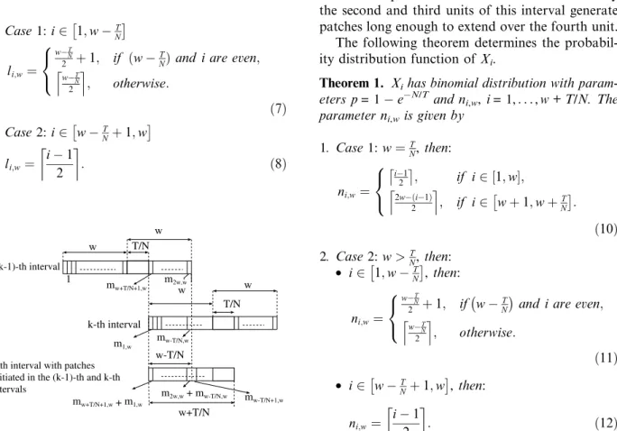
For example, Fig. 4(a) shows P[Xi=k] for N= 50, T= 103 and k= 1, 2. The value of

P[Xi=k] is constant for the sub-interval [1,w T/N] since ni;w¼ wT₂=N

l m

for these units. In

Fig. 4(b) the value of P[Xi=k], for N= 100, w + T/N

2

1 3 4 w

patch

w + T/N 2

1 3 4

patch

6 5

arrival arrival

w + T/N 2

1 3 4

patch

6 5 arrivals

patch

w w

(a) (b) (c)

Fig. 3. Concurrent streams in the fourth unit of an interval [1,w+T/N]: (a) one arrival in the second unit, (b) one arrival in the third unit, (c) one arrival in the second and third units.

Table 2

Size of the sub-intervals for diﬀerent values ofN

N [1,wT/N] [wT/N+ 1,w+T/N]

10 56% 44%

25 72% 28%

50 80% 20%

100 86% 14%

200 90% 10%

400 93% 7%

(8)

T= 103andk= 1, 2, oscillates between two values for the sub-interval [1,wT/N] (ni,w is computed

from Eq. (11)). In both ﬁgures, at the end of the interval, we see thatP[Xi=k] shows more

variabil-ity. As already explained, this behavior is due to the larger variability of the parameter ni,w in the

sub-interval [wT/N+ 1, w+T/N].

Based on the analysis presented above, we approximate the distribution of the number of con-current patches in the interval [1,w+T/N] by a binomial distribution with parameters p= 1 eN/Tand the expected value of ni,w. Note that the

larger N is, the more accurate our approximation tends to be since the variability of the parameter

ni,w tends to reduce. More formally, letXbe a

ran-dom variable which represents the number of con-current patches in the interval [1,w+T/N]. We thus approximate the distribution of X by a bino-mial distribution with parameters p= 1eN/T

andnw ¼

PwþT=N i¼1 ni;w wþT=N

.

Finally, we have to consider the full-object multi-casts to obtain the distribution of the total number of concurrent streams required by Patching. It is the sum of the concurrent patches and the concurrent full-object multicast streams. LetZdenote the ran-dom variable which represents the total number of concurrent streams.Zhas the same distribution of

X shifted to the right by MC. As previously

men-tioned, the number of concurrent full-object multi-casts is approximated by MC¼ N=

2Nþ1 p

. Thus it follows thatP(Z6MC1) = 0. The probability

distribution function ofZis given by Eq. (14). We note that bothXandZonly depend on the param-etersNandTof the objectO

PðZ6kÞ ¼ 0;

06k6v1;

Pk

j¼v

nw

l

ð1eN=T_Þl

ðeN=T_Þnwl_;

v6k6nwþv;

8 > > > > > <

> > > > > :

ð14Þ where nw¼

PwþT=N i¼1 ni;w wþT=N

, v_¼MC¼N=

2N_þ1 p

, andl=jv.

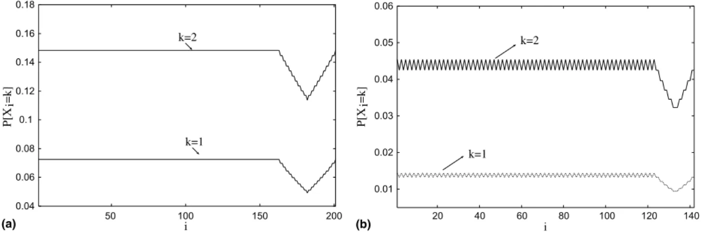
Our model is closer to the original continuous model of Patching as the value of d decreases. In the limit, whend_!0, our model becomes identical to the original Patching model since users have immediate service. Now, we deﬁne two criteria to estimate a value ford. The ﬁrst is based on the prob-ability of more than one arrival in a unit of lengthd, and the second is based on the relative error between the expected value of Z and the average bandwidthBcomputed from Eq.(3).

Fig. 5 shows the probability of more than one arrival in a unit of length dfor several values of N

and T. Recall that T=D/d. From this ﬁgure we note that, forTP104, the probability of more than one arrival is smaller than 104for all values of N. Let us now evaluate the second criterion. The expectation ofZis given by

E_½Z_¼nwð1eN=TÞ þN=

2N_þ1 p

: ð15_Þ

We deﬁne the relative error between E[Z] andBas

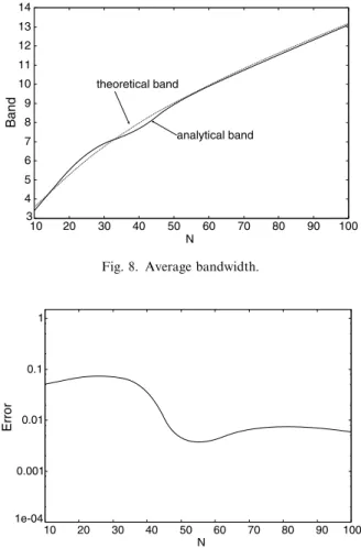
EMB¼jBE½Zj_B . InFig. 6, we plot the relative error as a function ofTforN= 10, 25, 40, 75 and 100. We also show the complementary cumulative distribu-tion funcdistribu-tion (CCDF) ofZforN= 100 and several values of T. As already expected, the value of the

0.01 0.02 0.03 0.04 0.05 0.06

20 40 60 80 100 120 140

k=1

k=2

i 0.04

0.06 0.08 0.1 0.12 0.14 0.16 0.18

50 100 150 200

k=2

k=1

P[X

i=k]

(a)

P[X

i=k]

(b) _i

(9)

relative error decreases as the value of Tincreases. However, we note that the relative error has no signiﬁcant reduction for T> 104. Moreover, the CCDFs ofZare practically the same forTP104.

3.2. Multiple objects

A multimedia server usually services client requests for more than one object simultaneously and so the bandwidth usage distribution in this case plays an important role in the overall system conﬁguration.

In the last subsection, we show that the random variable Z, which represents the distribution of the number of concurrent streams for a single object, depends on two parameters: N and T. Note that we can consider T equal to a constant value com-puted in accordance with the two criteria previously deﬁned (see last subsection). IfTis set to a constant, the random variable Z depends exclusively on the parameterN.

Assume that there arendiﬀerent objects stored in the multimedia server. These objects have lengths

D1,D2,. . .,Dn, respectively. We may compute the

corresponding values T1,T2,. . .,Tn using the two

criteria previously deﬁned (see last subsection). Notice that T= max{T1,T2,. . .,Tn} may be used

for all thesen objects. This is because the larger T

is, the more accurate our model becomes, as already observed. We emphasize that to considerTas a con-stant and the same for all objects stored in the server does not mean that the objects must have a same lengthD, as we explain in the following.

We know thatT=D/d(seeTable 1for reference). Since we propose an analytical model and have a steady-state analysis, the value ofDdoes not aﬀect the real distribution. For example, in Fig. 7 we plot the CCDF curves (obtained via simulation) for an object of popularity N= 5 and considering

D= 100 min, 200 min, 500 min. We may see that the curves are the same. Similar behavior is observed

0.001 0.01 0.1

1000 10000

N=10 N=25

N=40

N=100 N=75

T

EMB

0 0.2 0.4 0.6 0.8 1

0 5 10 15 20 25 k

P[ Z > k

]

T=103

T=105, 2x105

T=104

(b) (a)

Fig. 6. Analysis of the value ofT: (a) relative error, (b) CCDF ofZ.

0 0.2 0.4 0.6 0.8 1 1.2

0 5 10 15 20

P[ Z > k ]

k

N=5 and D=100 min, 200 min, 500 min

Fig. 7. Distribution ofZforN= 5 and diﬀerent values ofD.

1e-11 1e-10 1e-09 1e-08 1e-07 1e-06 1e-05 0.0001 0.001 0.01

10 20 30 40 50 60 70 80 90 100 N

P[A>1]

T=104

T=105

T=106 T=103

(10)

for other diﬀerent values ofDand a same Nin the interval [10, 100].

Still we consider that then objects stored in the multimedia server have the same play rate. This is a quite common assumption of previous work (e.g., [29,33,18,15]) and is mainly supported by recent researches (e.g., [41,11]) which analyze real media server workloads.

Let YNbe the random variable that denotes the

number of concurrent patches due to the delivery of all objects of popularity N, N2{1,. . .,Nmax},

where Nmax is the highest object popularity value

in the server. Once we consider T as a constant and the same for all objects stored in the server, we have thatYNis a sum of identical binomial

ran-dom variables, with parameters p= 1eN/T _and

nN;w ¼mN P

wþT=N i¼1

ni;w

wþT=N

l m

, where mN denotes

the total number of objects of popularityN in the server[37].

Now we want to estimate the total required bandwidth due to patches in the multimedia server. LetYbe the random variable that denotes the total number of concurrent patches due to the delivery of all objects in the server. Then,Yis the sum of poten-tiallyNmaxbinomial random variables with diﬀerent

parameters. There is no closed-form solution for the distribution of this sum. However the distribution of Y may be calculated based on the convolution of the individual probability mass functions (PMFs) of YN, for N= 1,. . .,Nmax. This convolution may

be eﬃciently implemented with the Fast Fourier Transform[38].

The total number of concurrent streams is the sum of patches and full-object multicasts. The num-ber of full-object multicasts is equal to f _¼

PNmax

N¼1pmffiffiffiffiffiffiffiffi₂N_NN_þ₁. LetSbe the random variable that

rep-resents the total number of concurrent streams due to the delivery of all objects in the server. The distri-bution of S is the distribution of Y shifted to the right by f. Similarly to the analysis in the single object case, the shift is because we assume that the total number of full-object multicast streams is a constant given byf, which corresponds to the sum of all individual multicast components related to the objects in the server. Thus it follows that

P(S6f1) = 0.

4. Results

In this section, we validate our analytical model using simulation and show for instance how we may practically use the bandwidth usage

distribu-tion we obtained (i) to allocate bandwidth to pro-vide a given level of QoS, (ii) to estimate the impact on QoS when some system parameters dynamically change, and (iii) to conﬁgure the over-all system. We mention that the simulation results are obtained using the modeling environment Tangram-II[39,40], and have 95% conﬁdence inter-vals that are within 5% of the reported values. Client arrivals are generated according to a Poisson process and the media objects are 100 min long. Lastly, since Patching is a multicast technique, we mainly focus on the values of N in the range of 10–100.

Tangram-II is an environment for computer and communication system modeling and experimenta-tion developed at Federal University of Rio de Janeiro (UFRJ), with participation of UCLA/ USA, for research and educational purposes. It combines a sophisticated user interface based on an object oriented paradigm and new solution tech-niques for performance and availability analysis. The user speciﬁes a model in terms of objects that interact via a message exchange mechanism. Once the model is compiled, it can be either solved analyt-ically, if it is Markovian or belongs to a class of non-Markovian models, or solved via simulation. There are several solvers available to the user, both for steady state and transient analysis.

The organization of this section is detailed in the following. Section 4.1 shows the model accuracy and how to use the bandwidth distribution of a sin-gle object to dynamically reserve a given number of channels for a group of clients. In Section 4.2, we study the behavior of the bandwidth distribution of a single object considering diﬀerent values of the threshold windowwfor a given object popular-ity. We evaluate the required bandwidth when the server operates using a window that is not the optimal one and quantify the impact on QoS. This analysis is motivated by the fact that the computa-tion of the optimal window to be used at time t

depends on the accurate estimation of the arrival rate k _{at time} _t_{. Finally, Section} _4.3 _{evaluates the}

use of the bandwidth distribution of multiple objects to compute the total server capacity to achieve a given level of QoS to the clients.

4.1. Model validation and bandwidth reservation

To evaluate the accuracy of our model we set

(11)

ﬁrst criterion, we compare the average bandwidthB, computed from Eq.(3)(theoretical), with that com-puted from our model E[Z] (analytical – Eq.(15)). We calculate the relative error from Error_¼ jBE½Zj

B .Fig. 8showsBandE[Z], andFig. 9presents the obtained relative errors for 106N6100. We may see that they lie between 102 _{and 10}3 _and

are thus satisfactory. In Table 3 we illustrate the parameters p and nw considering some values

ofN.

As for the second criterion, we compute the MSE values for the single object and multiple objects

cases from MSEsingle¼ PM

i¼1jð1FZðzÞÞð1FZsðzÞÞj 2

M and

MSEmultiple¼ PM

i¼1jð1FSðsÞÞð1FSsðsÞÞj 2

M , respectively, whereMis the number of samples and the subscript

sof the random variablesZandSis used to refer to simulation results. Recall thatZandSrepresent the number of concurrent streams for the single object and multiple object cases, respectively. Fig. 11

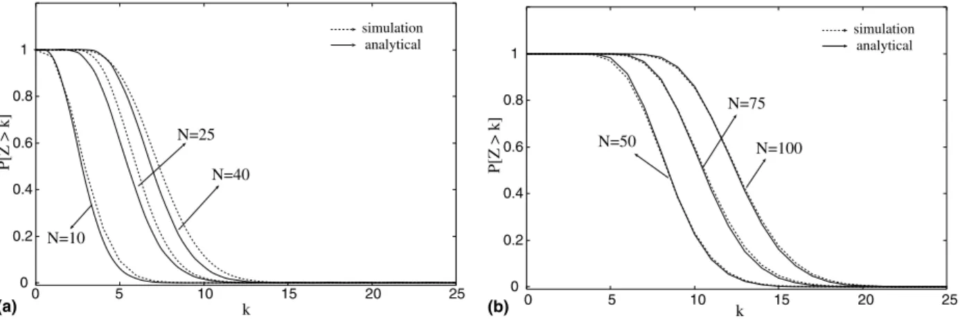
shows the complementary cumulative distribution function (CCDF) of the number of concurrent streams considering N= 10, 25, 40, 50, 75 and 100. In this ﬁgure, we have both analytical and sim-ulation results (solid and dotted lines, respectively). And inFig. 10we have the computed MSE values for 106N6100.

Note that the values of MSE are all smaller than 103_{. This indicates that the analytical results are}

satisfactorily close to those obtained using simula-tion. From Figs. 10 and 11 we can observe that the accuracy of the model tends to increase with the value ofN. In other words, the proposed model tends to be more accurate for the most popular objects, i.e., the objects that will signiﬁcantly impact on the server bandwidth. We stress that this is a ten-dency that has been conﬁrmed by the overall results obtained in the experiments. Therefore we may not state that for any given value ofN, the larger it is, the more accurate the model is.

We recall that we use the expected value ofni,wto

parameterize the binomial distribution. The parameter

ni,wexhibits more variability in the sub-interval [w T/N+ 1,w+T/N] as shown in Section 3.1. Then, the accuracy of the model is mainly aﬀected by the size of the sub-interval [wT/N+ 1,w+T/N] and the

3 4 5 6 7 8 9 10 11 12 13 14

10 20 30 40 50 60 70 80 90 100 theoretical band

analytical band

Band

N

Fig. 8. Average bandwidth.

1e-04 0.001 0.01 0.1 1

10 20 30 40 50 60 70 80 90 100

Error

N

Fig. 9. Relative errors for average bandwidth.

Table 3

Values of parameterspandnw

N p nw

10 9.99e04 1401

25 2.50e03 1057

40 3.99e03 890

50 4.98e03 816

75 7.47e03 692

100 9.95e03 613

0 20 40 60 80 100

MSE

N 1e-05

1e-04 0.001 0.01

(12)

variability ofni,win this subinterval. The size of the

sub-interval [wT/N+ 1,w+T/N] decreases with the value ofN. However, the variability ofni,wdoes

not always decrease with the value ofN. For exam-ple, the coeﬃcient of variation ofni,wforN= 10 is

smaller than that for N= 25. The behavior of the MSE is a consequence of the variability ofni,w.

Fig. 11 also demonstrates that, in general, the analytical results underestimate the simulation ones. The explanation for this result is that we use average values to determine the multicast component (MC)

as well as to calculate the parameternwof the

bino-mial distribution. Consider two binobino-mial random variables Y1 and Y2 with the same parameter p

(probability of success) and distinct parametersm1

andm2(number of trials), wherem1<m2. We have

thatY1always underestimatesY2[37]. In our model

we approximate the number of concurrent patches by a binomial random variableX with parameters

pand the expected value ofni,w. We recall that the

number of patches in the ith unit of the interval [1,w+T/N] is represented by the random variable

Xi with parameters p and ni,w. We thus have the

condition stated above, i.e., the random variable

X underestimates the random variables Xi with ni,w>nw. Similarly, the average value provided by MCunderestimates some of the real instantaneous

values of the multicast component.

In Fig. 12 we have the CCDF for the multiple object case. In this example we considered the same six objects analyzed in Fig. 11. The analytical and simulation curves are quite close to each other, and the MSE is equal to 2.32e04 which is quite satisfactory. We may also note that this value is smaller than the values obtained for N640. This occurs because although the bandwidth consumed

for delivery of a given object may significantly vary over time, the total bandwidth (i.e., the sum of indi-vidual bandwidths) to deliver a large number of objects simultaneously will have lower coefficient of variation over time for independently requested objects and fixed client request rate [6,37].

In the following we focus on applications con-cerning the single object case and leave the discus-sion of the multiple object case for Section4.3.

Using our analytical results we have the analysis that follows. With the distribution of the number of concurrent streams we can reserve bandwidth for a group of clients such that these clients may have a very low probability of not being immediately served. Assume, for example, that we reserve k

channels in the server for a group of users retrieving object O such that P[Z>k] = 103, that is, the probability of the number of concurrent streams be larger than k is equal to 103. The value of k

0 0.2 0.4 0.6 0.8 1

0 5 10 15 20 25

N=50 _N=100

N=75

0 0.2 0.4 0.6 0.8 1

0 5 10 15 20 25

N=10

N=25

N=40

k

P[Z > k]

(a) (b)

P[Z > k]

simulation analytical

k

Fig. 11. CCDF of the number of concurrent streams for a single object: (a)N= 10, 25, 40; (b)N= 50, 75, 100.

0 0.2 0.4 0.6 0.8 1

0 20 40 60 80 100 120 140 simulation analytical

P[S > k

]

k

(13)

may be easily obtained from Table 4 for N= 25, 50, 100. This table shows the estimated band-width (EB), the probability of the number of con-current streams to exceed the estimated bandwidth (P[Z> EB]), and the needed increase with respect to the average bandwidth (NI) for N= 25, 50, 100. The values of EB in the ﬁrst line of the table are equal to the average bandwidth computed from Eq.(3). We may conclude that if bandwidth reserva-tion is based on the average bandwidth, the proba-bility of the number of concurrent streams to exceed the reserved value is greater than 0.38 (Table 4) for all values ofN. In others words, the probability that a client arrives and has to wait until the server may allocate a channel for him is equal to 0.38 for

N= 50. This means that clients have a high proba-bility of waiting until the server may allocate a channel to serve them. We note that for N= 25, approximately 50% of the clients will not be imme-diately served.

4.2. Analysis for different values of the threshold window

Consider a server that dynamically estimates the value of k _{and then determines the threshold}

win-dow to be used in accordance with the value of the optimal window (Eq. (2)). Suppose that the value initially obtained for Nis equal to 75. From

Fig. 13, the bandwidth needed in order to have

P[Z>k]102 _{is 17. Now assume that the value}

of k _{changes and the server does not immediately}

detect it. The server continues to operate with the optimal window determined for N= 75 and keeps the same previously reserved bandwidth. Consider-ing this scenario, we would like to answer the two following questions: (i) What is the quality of service provided by the previously reserved band-width to the clients accessing the server now? (ii)

What is the impact of operating with a threshold window that is not the optimal one? And what are the bandwidth requirements of this threshold window?

Let us analyze the ﬁrst question. In our example we assume that N= 75, the reserved bandwidth is equal to k channels, and the threshold window is equal to the optimal value computed for N= 75. If the bandwidth and the threshold window are computed in accordance with a popularity equal to 75 and the arrival rate k _{increases (decreases),}

we can observe from Fig. 13 that the probability of the number of concurrent streams to be greater than the reserved value increases (decreases). This is an expected result, but using our model we can precisely quantify the QoS oﬀered to the users when their arrival rate changes and the server does not detect it. Suppose, for example, that the number of reserved channels is 17. We have P[Z> 17] = 6.8e03 for N= 75. If k _{decreases so that} _N_{= 50}

and the server does not detect it, we have that

P[Z> 17] = 1.1e04. Thus, the probability that

Table 4

Bandwidth evaluation forN= 25, 50, 100

N= 25 N= 50 N= 100

EB P[Z> EB] NI EB P[Z> EB] NI EB P[Z> EB] NI

6 4.9e01 – 9 3.8e01 – 13 4.1e01 –

7 2.7e01 16.67% 10 2.3e01 11.11% 14 2.7e01 7.69% 8 1.3e01 33.33% 11 1.2e01 22.22% 15 1.6e01 15.38% 9 5.2e02 50.00% 12 5.5e02 33.33% 16 8.9e02 23.08% 10 1.8e02 66.67% 13 2.3e02 44.44% 17 4.6e02 30.76% 11 5.7e03 83.33% 14 8.9e03 55.56% 19 9.6e03 46.15% 12 1.6e03 100.00% 15 3.1e03 66.67% 21 1.5e03 61.54% 13 4.1e04 116.67% 17 3.1e04 88.89% 22 5.6e04 69.23%

1e-05 0.0001 0.001 0.01 0.1 1

10 11 12 13 14 15 16 17 18 19 20 21 22 23 24 25

k

P[Z > k]

N=100

N=75

N=50

(14)

we need more channels, besides the reserved ones, decreases by one order of magnitude. On the other hand, if k _{increases so that} _N_{= 100, we have that} P[Z> 17] = 7.2e02, i.e., the probability increases by one order of magnitude. (Note that the band-width distributions for N= 50 and N= 100 in

Fig. 13 were computed using the optimal window deﬁned forN= 75.)

Fig. 14presents another example that illustrates the quality of service perceived by the clients when the arrival rate changes. In this example we set an initial value for the arrival rate and evaluate the QoS as the arrival rate increases. InFig. 14(a) the server is initially conﬁgured for N= 10 and in

Fig. 14(b) it is initially conﬁgured for N= 50. We note that, for N= 10 and N= 50, an increase of approximately 20% in the arrival rate does not

sig-nificantly affect the quality offered to the clients. The same behavior is observed for other values of

Nin the interval [10, 100].

Now, we present the analysis of the second ques-tion.Fig. 15shows the distribution of the number of concurrent streams Z when the threshold window varies around 20% of its optimal value for N= 50 andN= 100. We may notice that these distributions are quite similar. Hence, if the server does not detect changes in the value ofk_{, and consequently does not}

update the value of the threshold window, the required bandwidth for this non-optimal window is quite similar to that computed for the optimal one. In other words, the threshold window may vary within certain limits around the optimal win-dow value without signiﬁcantly aﬀecting the band-width requirements. Qualitatively similar results

0.0001 0.001 0.01 0.1 1

5 10 15 20 25 30 35 40 45 50 55

P[Z > k]

N P[Z > 5]

P[Z > 7]

P[Z > 8]

0.0001 0.001 0.01 0.1 1

50 60 70 80 90 100

P[Z > k]

N P[Z>12]

P[Z>14]

P[Z>17]

(a) (b)

Fig. 14. Quality of service as the value ofNincreases: (a) forN= 10:P[Z> 5] = 102_;_P[Z_{> 7] = 10}3_;_P[Z_{> 8] = 10}4_{, (b) for}_N_{= 50:} P[Z> 12] = 102_;_P[Z_{> 14] = 10}3_;_P[Z_{> 17] = 10}4_.

0 0.1 0.2 0.3 0.4 0.5 0.6 0.7 0.8 0.9 1

0 5 10 15 20 25

optimal window window 20% smaller than the optimal one

window 20% larger than the optimal one

k

0 0.1 0.2 0.3 0.4 0.5 0.6 0.7 0.8 0.9 1

0 5 10 15 20 25

window 20% smaller than the optimal one

optimal window

window 20% larger than the optimal one

k

P[Z > k]

(a) (b)

(15)

are obtained for other values of N in the interval [10, 100].

In summary, we are able to predict the band-width requirements for a given object, or for a group of clients, in order to guarantee a certain quality of service based on the distribution of the number of concurrent streams. This distribution also allows us to predict the quality of service when the client arrival rate changes and the server does not detect it quickly. Moreover, increases of 20% in the arrival rate do not considerably impact on the quality oﬀered to the clients. Another important point is related to the value of the threshold win-dow. We observe that changes around 20% of the optimal window value do not signiﬁcantly impact on the distribution.

4.3. Server configuration

As already mentioned, the distribution of the number of concurrent streams in the case of the multiple objects may be used, for example, to figure the server. To exemplify this point, we con-sider four specific scenarios based on the real case studies of [41]. They showed that the distribution of access frequencies for all media objects of two educational servers (BIBS and e-Teach) can be approximated by a concatenation of two Zipf distri-butions. The first Zipf is used for the most popular objects and the second for the least requested objects. We only consider the first Zipf distribution since the access frequency of the least requested objects is very low and therefore has little or almost no influence on server bandwidth. The scenarios we

studied are summarized inTable 5. It presents the number of objects in each scenario for each value ofN. Each scenario has a distinct value of skew fac-tor z and we have the most popular 50–55 min media objects of the BIBS server.

Fig. 16(a) shows the probability of the total num-ber of concurrent streams to exceed the average ser-ver bandwidth. The aser-verage serser-ver bandwidth is equal to the sum of the individual average band-widths for the objects being delivered (computed from Eq. (3)). Fig. 16(b) shows the needed incre-ment with respect to the average server bandwidth to achieve a given probability for a client not being immediately served. We can observe that the probability of exceeding the average server band-width is greater than 0.18 for all scenarios. The needed increase in bandwidth goes from 32% (Scenario 1 and P[S>k= 104]) to 6% (Scenario 4 andP[S>k= 102]). The experiments also show that the more objects we have, the smaller is the increase in the average server bandwidth to reach a given level of QoS, as similarly observed in

[6,33]. Table 5

Number of objects in each scenario

N Scenario 1, z= 0.60

Scenario 2, z= 0.55

Scenario 3, z= 0.80

Scenario 4, z= 0.65

100 1 2 2 4

75 1 2 2 3

50 1 2 2 3

40 1 1 2 3

25 1 1 2 3

10 1 1 2 2

0.16 0.18 0.2 0.22 0.24 0.26

6 8 10 12 14 16 18

P[S > Average server bandwidth]

Number of Objects

0 5 10 15 20 25 30 35

6 8 10 12 14 16 18

Number of Objects

Needed Increase (%)

10-4 10-3

10-2

(a) (b)

Fig. 16. Analysis of the multiple object case. (a) P[S> average server bandwidth], (b) % increase in server bandwidth to have P[S>k] = 102

, 103 or 104

(16)

5. Conclusions and ongoing work

In this work, we developed a very simple and pre-cise analytical model to calculate the distribution of the number of concurrent streams generated by the Patching technique, or equivalently, the server band-width usage distribution. In the case of the single object, we showed that the bandwidth usage distribu-tion can be accurately modeled in the form of a closed-form solution as a binomial distribution. Only two system variables are required to compute the parameters of the binomial distribution: the mean client arrival rate and the media object length. For the multiple object case, the distribution is a sum of independent binomial random variables which may be easily implemented using Fast Fourier Transform. Through simulations and analytical analysis we val-idate our model and illustrated how our results may be practically used in real project designs to mainly provide quality of service to system clients. Some of our main observations were:

• _{We may easily employ our results to dynamically}

allocate server bandwidth to guarantee a certain level of QoS for a group of clients retrieving an object from the multimedia server.

• _{In the case of the single object, we observed that}

the probability of exceeding the well-known aver-age value is signiﬁcant (0.4). This means that the QoS is severely aﬀected if bandwidth reserva-tion is based on average values.

• _{Using our results we may easily predict the QoS if}

the arrival rate changes and the server is not able to detect it immediately. For instance, we observed that variations below 20% do not severely impact on the system QoS. Similarly, we noticed that the Patching window size may also vary around 20% of its optimal value without signiﬁcantly aﬀecting the bandwidth distribution.

• _{In the case of multiple objects and considering}

real-case-based scenarios, we observed that to guarantee a low probability of a client not being served immediately (104), we need a server bandwidth which is 15–32% larger than the well-know average value. This conﬁrms the usefulness of our results to guarantee system QoS.

As an extension of this work, we include the evaluation of the impact on the server bandwidth usage distribution of both a limited client band-width and client interactive behavior. We also plan

to investigate the distribution considering other than a Poisson client arrival process.

Appendix A

Proof of Lemma 1. We show by mathematical

induction that Eqs. (5) and (6) are correct and thereforeLemma 1is true.

• _{Case 1:}_i_{= 1, 2,} . . .,w. Base case

It is easy to verify that fori= 1 and allw, we have thatm1,w= 0. This agrees with the result of Eq.(5).

Inductive hypothesis

First, assume that the lemma is true for 16i6k, where k is even, i.e., k= 2c and c₂{1, 2,_{. . .}}. We therefore may write the following: m2c;w ¼

2c1 2

¼c, andm2c1;w¼ 2c₂11

¼c1.

Second, assume that the lemma is true for 16i6k, where k is odd, i.e., k= 2c1 and

c₂{1, 2,. . .}. We therefore may write the

follow-ing: m2c1;w¼ 2c₂11

¼c1, and m2c2;w ¼

2c21 2

¼c1.

We thus obtain the following relation from the inductive hypothesis: (i) If i is even, then

mi,w=mi1,w+ 1; (ii) ifiis odd, thenmi,w=mi1,w.

Evaluation of Eq.(5)for i + 1

We use the assumptions of the inductive hypothe-sis and prove that the result of Eq.(5)holds for

i+ 1. As before, letc₂{1, 2,_{. . .}}. Two cases must be considered:

– iis odd, theni+ 1 is even.

We havei= 2c1 andi+ 1 = 2c. We obtain

m2c;w¼ 2c₂1

¼cusing Eq.(5). Now using the result of the inductive hypothesis we have that

m2c,w=m2c1,w+ 1 =c1 + 1 =c.

– iis even, theni+ 1 is odd.

We havei= 2candi+ 1 = 2c+ 1. We obtain

m2cþ1;w ¼ 2cþ₂11

¼c using Eq. (5). Now using the result of the inductive hypothesis, we have thatm2c+1,w=m2c,w=c.

This completes the proof of Eq.(5).

• _{Case 2:}_i₌_w_{+ 1,} _w_{+ 2,} . . ., 2w. Base case

It is easy to verify that for w= 1 andi= 2, we have thatm2,1= 1. This agrees with the result of

Eq. (6).

Inductive hypothesis

Let c1 and c22{1, 2,. . .}. Two cases must

be considered:

(17)

i.e., w= 2c1, we obtain: m2c2;2c1¼ 4c12₂c2þ1

¼ 2c1c2þ1, and m2c21;2c1¼ 4c12₂c2þ2

¼2c1

c2þ1. For w odd, i.e., w= 2c11, we

obtain: m2c2;2c11¼ 4c1222c2þ1

¼2c1c2, and m2c21;2c11¼ 4c12₂2c2þ2¼2c1c2.

– Now, assume that the lemma is true for 16i6k, where k is odd, i.e., k= 2c21.

For w even, i.e., w= 2c1, we obtain: m2c21;2c1 ¼ 4c12₂c2þ2

¼ 2c1 c2þ1, and

m2c22;2c1 ¼ 4c12c2þ₂ 2þ1

¼ 2c1c2 þ2. For w odd, i.e., w= 2c11, we obtain: m2c21;2c11 ¼ 4c12₂2c2þ2

¼ 2c1 c2, and

m2c22;2c11 ¼ 4c12₂2c2þ3 ¼ 2c1 c2 þ1.

We thus obtain the following relation from the inductive hypothesis: wheniis even, we have that

mi,w=mi1,w; when i is odd, we have that

mi,w=mi1,w1.

Evaluation of Eq.(6)for i + 1

We use the assumptions of the inductive hypoth-esis and prove that the result of Eq.(6)holds for

i+ 1. As before, let c1 and c22{1, 2,. . .}. Two

cases must be considered:

– i is odd, then i+ 1 is even. We have

i= 2c21 then i+ 1 = 2c2.

For w even, i.e., w= 2c1, we have m2c2;2c1¼ 2c1c2þ1 from Eq. (6). The result of

the inductive hypothesis gives: m2c2;2c1¼

m2c21;2c1¼2c1c2þ1.

For w odd, i.e., w= 2c11, we have m2c2;2c11¼2c1c2 from Eq. (6). The result

of the inductive hypothesis gives: m2c2;2c11¼ m2c21;2c11¼2c1c2.

– i is even, then i+ 1 is odd. We have i= 2c2

theni+ 1 = 2c2+ 1.

Forw even, i.e.,w= 2c1, we havem2c2þ1;2c1¼ 2c1c2from Eq.(6). The result of the

induc-tive hypothesis gives:m2c2þ1;2c1¼m2c2;2c11¼ 2c1c2þ11¼2c1c2.

For w odd, i.e., w= 2c11, we have m2c2þ1;2c11¼2c1c21 from Eq. (6). The

result of the inductive hypothesis gives:

m2c2þ1;2c11¼m2c2;2c111¼2c1c21.

This completes the proof of Eq. (6). _h

Appendix B

Proof of Lemma 2. We show that Eqs. (7)–(9) are correct and thereforeLemma 2 is true.

• _{Case 1:}_i_{2 ½}₁_;_wT N

We have that li,w=mi+w+T/N,w+mi,w, where

mi+w+T/N,w is the number of patches initiated in

the previous interval and mi,w is the number of

patches initiated in the current interval. Substi-tuting Eqs.(5) and (6)ofLemma 1in the expres-sion obtained forli,w, gives

li;w¼

2wðiþwþT=N1Þ 2

þ i₂1

¼ wT=N₂iþ1

þ i₂1

: ðB:1Þ

Now we consider the possible values for i and (wT/N) (even or odd):

– iand wT N

are even

li;w ¼

wT=N

2

i

2þ1þ

i

2¼

wT=N

2 þ1: ðB:2Þ – iis even andðwT

NÞis odd

li;w ¼

wT=N

2 þ 1 2 i 2þ i 2¼

wT=N

2

:

ðB:3Þ – iand wT

N

are odd

li;w¼

wT=N

2

i₂1þi₂1¼ w₂T=N

:

ðB:4Þ – iis odd and wT

N

_{is even}

li;w ¼

wT=N

2

i1

2 þ

i1

2 ¼

wT=N

2

:

ðB:5_Þ This completes the proof of Eq.(7).

• _{Case 2:}_i₂ _wT Nþ1;w

We have thatli,w=mi,w since all patches

initi-ated in the (k1)th interval have already ﬁnished. From Eq. (5) of Lemma 1 we have

li;w¼

i1

2

: ðB:6_Þ

• _{Case 3:}_i₂ _w_þ₁_;_w_þT N

We have thatli,w=mi,wsince all patches initiated

in the (k1)th interval have already ﬁnished. From Eq.(6) ofLemma 1we have

li;w¼

2w ði1_Þ 2

: ðB:7_Þ

(18)

References

[1] C.C. Aggarwal, J.L. Wolf, P.S. Yu, On optimal piggy-back merging policies for video-on-demand systems, in: Proc. 1996 ACM SIGMETRICS Conf. On Measure-ment and Modeling of Computer Systems, 1996, pp. 200– 209.

[2] K.A. Hua, Y. Cai, S. Sheu, Patching: a multicast technique for true video-on-demand services, in: Proc. 6th ACM Int. Multimedia Conference (ACM MULTIMEDIA’98), 1998, pp. 191–200.

[3] Y. Cai, K.A. Hua, An eﬃcient bandwidth-sharing technique for true video on demand systems, in: Proc. 7th ACM Int. Multimedia Conference (ACM Multimedia’99), 1999, pp. 211–214.

[4] Y. Cai, K.A. Hua, K. Hu, Optimizing patching performance, in: Proc. SPIE/ACM Conference on Multimedia Computing and Networking, January 1999.

[5] S. Sen, L. Gao, J. Rexford, D. Towsley, Optimal patching schemes for eﬃcient multimedia streaming, in: Proc. 9th Int. Workshop on Network and Operating Systems Support for Digital Audio and Video (NOSSDAV’99), 1999.

[6] D. Eager, M. Vernon, J. Zahorjan, Minimizing bandwidth requirements for on-demand data delivery, in: Proc. 5th Int. Workshop on Multimedia Information Systems (MIS’99), 1999, pp. 80–87.

[7] D. Eager, M. Vernon, J. Zahorjan, Optimal and eﬃcient merging schedules for video-on-demand servers, in: Proc. 7th ACM Int. Multimedia Conference (ACM Multimedia’99), 1999, pp. 199–202.

[8] D. Eager, M. Vernon, J. Zahorjan, Bandwidth skimming: a technique for cost-eﬀective video-on-demand, in: Proc. IS & T/SPIE MMCN’00, 2000, pp. 206–215.

[9] A. Bar-Noy, R.E. Ladner, Competitive on-line stream merging algorithms for media-on-demand, in: Proc. 12th Annual ACM-SIAM Symposium on Discrete Algorithms (SODA), 2001.

[10] E.G.C. Jr., P. Jelenkovic, P. Momcilovic, Provably eﬃcient stream merging, in: Proc. 6th Int. Workshop on Web caching and Content Distribution, Boston, MA, 2001.

[11] C. Costa, I. Cunha, A. Borges, C. Ramos, M. Rocha, J.M. Almeida, B. Ribeiro-Neto, Analyzing client interactivity in streaming media, in: Proc. 13th ACM Int. World Wide Web Conference, May, 2004, pp. 534–543.

[12] W.-T. Chan, T.-W. Lam, H.-F. Ting, W.-H. Wong, Competitive analysis of on-line stream merging algorithms, in: Proc. of the 27th Int. Symposium on Mathematical Foundations of Computer Science (MFCS), 2002, pp. 188– 200.

[13] K.C. Almeroth, M.H. Ammar, The use of multicast delivery to provide a scalable and interactive video-on-demand service, IEEE Journal on Selected Areas in Communications 14 (5) (1996) 1110–1122.

[14] A. Hu, Video-on-demand broadcasting protocols: a com-prehensive study, in: Proc. IEEE Infocom, 2001, pp. 508– 517.

[15] S. Viswanathan, T. Imielinski, Pyramid broadcasting for video-on-demand service, in: Proc. SPIE Multimedia Com-puting and Networking Conference, 1995, pp. 66–77. [16] L. Juhn, L. Tseng, Fast data broadcasting and receiving

scheme for popular video service, IEEE Transactions on Broadcasting 44 (1) (1998) 100–105.

[17] L. Juhn, L. Tseng, Harmonic broadcasting for video-on-demand service, IEEE Transactions on Broadcasting 43 (3) (1997) 268–271.

[18] K. Hua, S. Sheu, Skyscraper broadcasting: a new broad-casting scheme for metropolitan video-on-demand systems, in: Proc. ACM SIGCOMM, 1997, pp. 89–100.

[19] J.-F. Paris, S.W. Carter, D.D.E. Long, A low bandwidth broadcasting protocol for video on demand, in: Proc. IEEE Int. Conference on Computer Communications and Net-works (IC3N’98), 1998, pp. 690–697.

[20] J.-F. Paris, S.W. Carter, D.D.E. Long, A hybrid broadcast-ing protocol for video on demand, in: Proc. SPIE Multi-media Computing Networking Conference (MMCN’99), 1999, pp. 317–326.

[21] J.-F. Paris, S.W. Carter, D.D.E. Long, A simple low-bandwidth broadcasting protocol for video on demand, in: Proc. 8th Int. Conference on Computer Communications and Networks (IC3N’99), 1999.

[22] Y. Guo, K. Suh, J. Kurose, D. Towsley, P2cast: peer-to-peer patching scheme for VoD service, in: Proc. 12th World Wide Web Conference (WWW-03), 2003, pp. 301–309.

[23] M.K. Bradshaw, B. Wang, S. Sen, L. Gao, J. Kurose, P. Shenoy, D. Towsley, Periodic broadcast and patching services – implementation, measurement and analysis in an Internet streaming video testbed, ACM Multimedia Journal 9 (1) (2003) 78–93.

[24] D. Guan, S. Yu, A two-level patching scheme for video-on-demand delivery, IEEE Transactions on Broadcasting 50 (1) (2004) 11–15.

[25] Y.W. Wong, J.Y.B. Lee, Recursive patching – an eﬃcient technique for multicast video streaming, in: Proc. 5th International Conference on Enterprise Information Systems (ICEIS) 2003, Angers, France, 2003, pp. 23–26.

[26] Y. Cai, K. Hua, Sharing multicast videos using patching streams, Journal of Multimedia Tools and Applications 21 (2) (2003) 125–146.

[27] Y. Cai, W. Tavanapong, K. Hua, Enhancing patching performance through double patching, in: Proc. Int. Conf. on Distributed Multimedia Systems, Miami, FL, USA, 2003, pp. 72–77.

[28] E. de Souza e Silva, R.M.M. Lea˜o, M.C. Diniz, The required capacity distribution for the patching bandwidth sharing technique, in: Proc. IEEE Int. Conference on Communica-tions (ICC 2004), 2004.

[29] A. Bar-Noy, G. Goshi, R.E. Ladner, K. Tam, Comparison of stream merging algorithms for media-on-demand, in: Proc. Multimedia Computing and Networking (MMCN’02), San Jose, CA, 2002, pp. 18–25.

[30] L. Gao, D. Towsley, Supplying instantaneous video-on-demand services using controlled multicast, in: Proc. IEEE Multimedia Computing Systems, 1999, pp. 117– 121.

[31] Y. Cai, K. Hua, K. Vu, Optimizing patching performance, in: Proc. SPIE/ACM Conference on Multimedia Computing and Networking, 1999, pp. 204–215.

[32] D.L. Eager, M.C. Ferris, M. Vernon, Optimized regional caching for on-demand data delivery, in: Proc. ISET/SPIE Conf. Multimedia Computing and Networking (MMCN’99), 1999, pp. 301–316.

(19)

[34] A. Bar-Noy, R.E. Ladner, Eﬃcient algorithms for optimal stream merging for media-on-demand, SIAM Journal on Computing 33 (5) (2004) 1011–1034.

[35] S.M. Ross, Stochastic Processes, second ed., John Wiley & Sons, Inc., New York, 1996.

[36] L. Kleinrock, Queueing Systems, Theory, vol. 1, John Wiley & Sons, New York, 1975.

[37] K.S. Trivedi, Probability and Statistics with Reliability, Queuing and Computer Science Applications, second ed., John Wiley & Sons, Inc., New York, 2002.

[38] E.O. Brigham, The Fast Fourier Transform and Its Appli-cations, Prentice-Hall, Inc., New Jersey, 1988.

[39] R.M.L.R. Carmo, L.R. de Carvalho, E. de Souza e Silva, M.C. Diniz, R.R. Muntz, Performance/availability modeling with the TANGRAM-II modeling environment, Perfor-mance Evaluation 33 (1998) 45–65.

[40] E. de Souza e Silva, R.M.M. Lea˜o, The Tangram-II environment, in: Proc. 11th Int. Conference TOOLS2000, 2000, pp. 366–369.

[41] J.M. Almeida, J. Krueger, D.L. Eager, M.K. Vernon, Anal-ysis of educational media server workloads, in: Proc. 11th Int. Workshop Network and Operating Systems Support for Digital Audio and Video (NOSSDAV’01), 2001, pp. 21–30. [42] E. de Souza e Silva, R.M.M. Lea˜o, B. Ribeiro-Neto, S.

Campos, Performance issues of multimedia applications, Lecture Notes in Computer Science 2459 (2002) 374–404. [43] Huadong Ma, K.G. Shin, Multicast video-on-demand

ser-vices, ACM SIGCOMM, Computer Communication Review 32 (1) (2002) 31–43.

[44] K.A. Hua, M.A. Tantaoui, W. Tavanapong, Video delivery technologies for large-scale deployment of multimedia appli-cations, Proceedings of the IEEE 92 (9) (2004) 1439–1451. [45] B. Wang, S. Sen, M. Adler, D. Towsley, Optimal proxy

cache allocation for eﬃcient streaming media distribution, IEEE Transactions on Multimedia (2004) 1726–1735.

[46] X. Zhang, J. Liu, B. Li, Tak-Shing P. Yum, CoolStreaming/ DONet: a data-driven overlay network for eﬃcient live media streaming, in: IEEE Infocom, 2005.

Carlo K. da S. Rodrigues received the B.Sc. in Electrical Engineering from Federal University of Paraiba in 1993 and the M.Sc from IME in 2000. He has been D.Sc. Student from Federal Uni-versity of Rio de Janeiro of System Engineering and Computer Science Pro-gram since 2002. He is also a member of the LAND – Laboratory for Modeling, Analysis and Development of Networks and Computer System. His current research interests are in the areas of computer networks and streaming media delivery.