ISSN: 1809-4430 (on-line) www.engenhariaagricola.org.br
1 Western Paraná State University/ Cascavel - Paraná, Brazil.
Received in: 8-15-2016
Doi:http://dx.doi.org/10.1590/1809-4430-Eng.Agric.v38n2p 188-196/2018
SPATIAL VARIABILITY OF THE WATER DEPTH APPLIED BY FIXED
SPRINKLER IRRIGATION SYSTEMS
Jorge T. Tamagi
1, Miguel A. Uribe-Opazo
2*, Marcio A. Vilas Boas
1, Jerry A. Johann
1,
Luciana P. C. Guedes
12*Corresponding author. Western Paraná State University / Cascavel - Paraná, Brazil. E-mail: [email protected]
KEYWORDS
compensating
sprinklers,
non-compensating
sprinklers, spatial
dependence.
ABSTRACT
The uniformity of water application is an important factor in the evaluation of sprinkler
irrigation systems. This uniformity depends on the type of sprinkler and its operating
conditions, such as the arrangement and spacing between the sprinklers in the area;
velocity and wind direction during the period of water application and the pressure
variation of the irrigation system. The objective of this study was to model, analyze and
compare the structure of spatial dependence, as well as the spatial variability of the water
depths applied by a sprinkler irrigation system with compensating and non-compensating
sprinklers, using geostatistical methods and measurements of accuracy or similarity
between the applied water depth maps. The experiment was carried out in an agricultural
area, in the city of Cascavel-Paraná-Brazil. A total area of 10 x 10 m was used, with 04
compensating and 04 non-compensating sprinklers installed at a height of 1.5 m. For each
type of sprinkler, water levels were measured in 100 collectors spaced 1 x 1 m in the
study area in 32 trials. On each test sprinkling was carried out for one hour. The
conditions of wind, temperature and air humidity were evaluated at the beginning of each
test and at 10-minute intervals with a climatological station. As the geostatistical analysis
showed the existence of directional trends, the coordinates were incorporated as
covariates to the linear spatial model in the study of the spatial dependence of the average
depth of the irrigation water for the two types of sprinklers. The spatial dependence
structure that best fits the data when using the compensating sprinklers was the Gaussian
model and when the non-compensating sprinklers were used, it was the exponential
model. The spatial variability maps of average irrigation water depth (mm) of the trials,
obtained by universal kriging, revealed that for both sprinklers there was an increase in
the mean level average values in the northwest-southeast direction (135
oin the azimuth
system) in the area under study, influenced by wind direction and velocity during the
execution of the experiment.
INTRODUCTION
Brazil is one of the countries with the largest reserves of fresh water on the planet (12% of the world total). Water resources have significant importance in the development of various economic activities, especially for the agribusiness sector that accounts for 23% of the Gross Do mestic Product (GDP) of Brazil.
Irrigation is an ancient technique that aims to provide the necessary amount of water to the plant at the mo ment it needs and in the exact amount. Since it is properly used, it has many benefits, such as increased
productivity, job creation, and profitable growth of rural producers (Oliveira et al., 2011; Souza et al., 2011).
Currently, Brazil is one of the ten countries with the largest irrigated area on the planet. According to the National Water Agency (ANA, 2017) the country has 6.95 million hectares using different irrigation techniques and can expand this area by 45% by 2030.
to Martins et al. (2008), is one of the most used methods in the last decades in Brazil, since, of the total area of irrigated vegetables, more than 90% are irrigated by sprinkling (Fravet & Cruz, 2007), which has contributed to increase both the irrigated area, as well as, the number of companies manufacturing irrigation equip ment (Rocha et al., 2005).
This information only illustrates the relevance that should be given to studies involving the evaluation of the distribution uniformity of the applied water levels depths of irrigation systems, considering that, the irrigation sector is the largest and most dynamic consumptive water use fro m the springs in Brazil, removing about 969 thousand liters of water per second, corresponding to 46% of all total water consumption (ANA, 2017).
According to Frizzone et al. (2011), the uniformity coefficients of water distribution have been the main evaluation method of an irrigation system, since they express, in a specific way, the variab ility of the irrigated water depth at the soil surface. This allows identify ing if the planning and operation of the system has been carried out correctly, in v iew of, the aspects related to sprinkler spacing, sprinkler type and the system operating pressure.
However, several surveys (Pair et al., 1969; Nogueira & Souza, 1987; Costa & Castro, 1993; A lves & Castro, 1995; Justi et al., 2010) have shown that the uniformity of water application is also affected by the wind velocity, because the wind causes a change in the distribution profile of the sprinkler and drags the droplets of smaller diameter. Generally, the higher the wind speed, the lower the coefficients of uniformity values. According to Bernardo (2006), the wind velocity less than 2.0 m s-1 does not generally affect this uniformity of water application, making it less significant when the spacing between sprinklers decreases.
Although, to visualize the spatial variability of the water depth applied by the irrigation system, is an important way to identify possible solutions to improve the uniformity of application. Thus, geostatistics is one of the most important and used methods of spatial analysis to study random variab les by means of probabilistic models, when it has the spatial location of the data (Uribe-Opazo et al., 2012; Robinson et al., 2013, Wendpap et al., 2015)
The objective of this study was to model, analy ze and compare the structure of spatial dependence, as well as, the spatial variability of water depths applied by a sprinkler irrigation system with compensating and non-compensating sprinklers, using geostatistical methods and measures of accuracy or similarity between the applied water depth maps.
MATERIAL AND MET HODS
Location of the sur ve y, sampling grid and arrange ment of the collectors or pluviometer
The experiment was carried out in the farm called
“Floricultura & Mercado de Plantas Cascavel”, north
region of the city of Cascavel-Paraná-Brazil, at 24o55’ 04”
South latitude, 53o 28’ 31” West longitude and altitude of
785 m. The climate of the region is temperate, mesothermic, super humid, sub-tropical, with average air temperature in January of 28.6C, and in Ju ly of 11.2C, with frost occurrence. In addition, in Cascavel, the average
annual precipitation is equal to 1940 mm and the annual average air relative hu mid ity is around 75% (Tamagi et al., 2016).
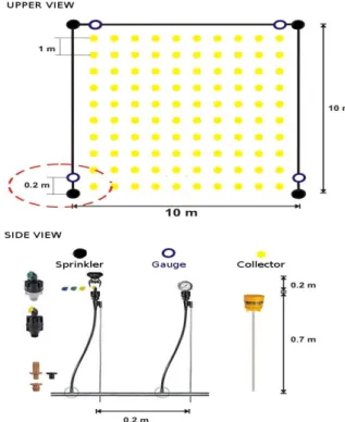
The mounted sprinkler system had the following equipment: 5 m³; water pu mp Sonar brand of 2 HP with 60 m.w.c. and Q = 4.5 m³ h-¹; 04 manometers of 0-10.5 Bar; filter; hydrometer; valves; tubing of black plastic lines of one inch in diameter; 04 co mpensating sprinklers and 04 non-compensating (blue nozzle, super 10, fro m NaanDan manufacturer) installed at 1.5 m height; 100 co llectors (with 80 mm in diameter and 102 mm in height, fro m the Fabrimar brand) fixed to metal rods, 70 cm fro m the soil surface; and a portable weather station La Crosse Technology to record the Agrometeorological conditions at the sprinkler test site.
Firstly, these equipments were installed in the total area of 10 x 10 m (Figure 1) with the 04 compensating sprinklers and the 100 co llectors distributed equidistantly in a 1.0 x 1.0 m grid (Figure 1). The collector lines
covered a distance greater than or equal to the emitter’s jet
range, which operated for 1 hour, in each of the 32 tests performed. For each test, the water volume of the collectors was measured by means of a graduated measuring cylinder, following the NBR ISO 7749-2 standard - Agricultural irrigation equipment - Rotating sprinklers and Part 2: Un iformity of d istribution and test methods (ABNT, 2000). After co mpleting the 32 tests with the compensating sprinklers, the same procedure was performed with the 04 non-co mpensating sprinklers. For each type of sprinkler used, the average value of the water depth (mm) of the 32 tests was considered as
variable for the analysis of spatial dependence.”
FIGURE 1. Layout of the arrangement of the collectors and sprinklers used in the experiment.
The agrometeorological variables, wind speed (WS) (m s-1), temperature (T) (°C) and relative hu midity
of these instruments was made, at the beginning of each sprinkler test and, then every 10 minutes until one hour of each test was completed.
For each type of sprinkler and for each of the variable (agro meteoro logical variables and the average water depth), a descriptive statistical analysis was carried out, whose objective was to describe briefly and compare the samples results obtained in all variables, among the types of sprinklers used. In order to verify if the agrometeorological conditions were statistically equal between the tests performed with co mpensating and non-compensating sprinklers, the t-Student hypothesis test was applied for independent samples, with a level of 5% of significance. Thus, if p-value < 0.05 (α=5%) then there is
significant statistical difference for each of the agrometeorological monitor variables; otherwise, the difference is not significant at 5% probability. The same hypothesis test was also applied to verify if the average of the water depths applied with the non-compensating and compensating sprinklers differed during the experiments.
Spatial anal ysis
The spatial dependence structure of the average water depth was also modeled for each type of sprinkler using geostatistical methods. To perform these analyzes, we considered a Gaussian stochastic process
Z
{Z(s), s ϵ S}, on whats
x
,
y
Tis the vector that represents a certain location in the study area, where and is the two-dimensional Euclidean space. Suppose the data Z(s) ={Z(s1),...,Z(sn)} of each process are recorded inknown spatial locations si (i = 1,...,n), and generated by the
model Z(si) = µ(si) + e(si) (Uribe-Opazo et al., 2012).
In this model, the mean µ(si) is the deterministic
term and e(si) is the stochastic term that depends on the
spatial location in which Z(si) was gotten. It was assumed
that the stochastic error e(si) has zero mean, that is, E[e(si)]
=0, and that the variation between points in space is determined by a covariance function Cov[e(si), e(su)] =
C(si, su) = σiu (Oliver & Webster, 2014).
The Gaussian linear spatial model can be written, in matrix notation, by [eq. (1)]:
Z = + ε, (1)
on that:
µ(s) = ; is the matrix of the design n x p; is
the vector p x 1 of the unknown parameters associated with the deterministic term (Monego et al., 2015, Schemmer et al., 2017); ε is the vector of random errors n x 1, with E(ε) = 0 (null vector) and covariance matrix Σ=[(σiu)]. It was assumed that Σ is a non-singular definite
positive matrix n x n and that Z has a normal p robability
distribution n-varied with mean vector and covariance matrix Σ, this is, Z ~ Nn ( , Σ) (De Bastiani
et al., 2015).
The parametric fo rm of the covariance matrix (Uribe-Opazo et al., 2012) be expressed by [eq. (2)]:
Σ= φ1In+ φ2R(φ3) (2)
on that,
φ1 is the nugget effect or variance error; In is an identity
matrix with dimension n x n; φ2 is the dispersion
covariance or variance; φ3 is a function of the practical
range (a) of the model; R(φ3), is a matrix, with dimension
n x n, that is a function of φ3. Being that R(φ3)=[(riu)] is a
symmetric matrix with its elements equal to: rii =1, to
i=1,...,n,
r
iu 1C
s
i,
s
u
2
to
2
0
and i ≠ u = 1,...,n, on that C(si, su) = C(hiu) is the covariance value between Z(si)and Z(su); and
0
iur
to
2
0
, i≠ u = 1,...,n. So,r
iuand C(si, su) depend on Euclidean distance hiu = ||si – su||between the points si and su .
The parametric fo rm of the covariance matrix Σ given in [eq. (2)], occurs for several stationary and isotropic processes (Guedes et al., 2013), in wh ich the covariance C(si, su) = C(hiu) can be expressed by the Matern functions’ family, given by [eq. (3)]:
3 3 1 2)
(
2
)
(
iu k k iu k iuh
K
h
k
h
C
, if hiu >0 and2 1
)
(
h
iu
C
, if hiu = 0 (3)on that:
) (k
is the gamma function,
is the modified Bessel function of third type, order , with fixed. When
k
1
2
andk
, this function [eq. (3)] corresponds to the exponential and Gaussian covariance functions, respectively.In covariance functions C(hiu), the variance of Z is
C(0) = φ1 + φ2 and is called the sill, and semivariance is
defined as γ(h)= C(0) – C(h) (Cressie, 2015).
The presence of directional tendency and anisotropy was evaluated initially by means of the Post-plot graph. In this graph, the values of the average depth in each type of sprinkler are classified according to the quartiles (the larger the range of values, the darker the color of the point in the gray scale).
The spatial dependence structure between the sample elements and the presence of anisotropy was identified through the construction of experimental semivariograms (o mnid irectional and directional), using the classical Matheron estimator [eq. (4)] to calculate the values of the semivariance as a function of distance (Grego et al., 2011).
( ) 1 i 2)]
Z(
)
Z(
[
.
)
(
2
1
)
(
ˆ
hs
ih
s
ih
h
N
N
(4)on that:
Z(sih), Z( )si is the regionalized variable in the positions si+h and si, respectively and
N
h
is the number of pairs of sampling points separated by vectors h, such thath
h
is the Euclidean distance between points (lag) (Oliver & Webster, 2014).
considered and
T3 2 1,
,
for a non-stationary and isotropic process, with a d irectional tendency in the x and y coordinates, where (De Bastiani et al., 2015). Considering the stochastic process Z=(Z(s1),...,Z(sn))T, onthat Z ~ Nn ( , Σ), the ML estimation method consists in
determining which is the estimated vector of [eq. (5)] which maximizes the logarith m of the likelihood function.
1
1 1
( ) log(2 ) log | | ( – X ) ( – X )
2 2 2
T
n
l
Z
Z
(5)In order to choose the model that best fits the data; we used the cross-validation technique and the Akaike criterion (Faraco et al., 2008; Lu et al. 2012; Robinson et al., 2013).
After the estimation of the parameters of the geostatistical model by the maximu m likelihood method, the average values of the water depth applied by sprinkler irrigation in non-sampled locations were estimated using the interpolator called universal kriging, used for processes in wh ich the determin istic term of the Gaussian spatial linear model is not constant. By means of this spatial estimation, the maps of the spatial variability of the
average water depth applied by sprinkler irrigation in the study area were elaborated.
The maps of the spatial variability of the average water depth were compared by the accuracy or similarity measures obtained by the error matrix: global accuracy ( ), Kappa concordance index ( ) and Tau concordance index ( ) (De Bastiani et al., 2012).
The software R (R Develop ment Core Team, 2016) and the geoR module (Ribeiro Jr. & Diggle, 2016) were used for the study of the spatial dependence of the data and the construction of interpolated maps to visualize the spatial variability of the average water depth for each one of the sprinklers.
RES ULTS AND DISCUSS IONS
Analysis of the Agromete or ological vari ables
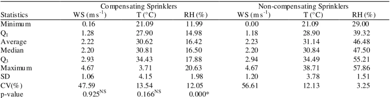
For each of the 32 tests and for each type of sprinkler (co mpensating and non-compensating) were realized 7 measurements of the agrometeorological variables (wind speed (WS) [m s-1], air temperature (T) [°C], air relative hu midity (RH) [%]), totaling 224 measurements, which are synthesized by the descriptive statistics in Table 1.
TABLE 1. Descriptive analysis of the agrometeorological variables: wind speed (WS), temperature (T) and relative humidity (RH), obtained during the 32 tests with compensating sprinklers and the 32 tests with non -compensating sprinklers.
Co mpensating Sprinklers Non-compensating Sprinklers
Statistics WS (m s-1) T (°C) RH (%) WS (m s-1) T (°C) RH (%)
Minimu m 0.16 21.09 11.99 0.00 21.09 29.00
Q1 1.28 27.90 14.98 1.18 28.90 39.32
Average 2.22 30.62 16.42 2.23 31.14 46.48
Median 2.20 30.81 16.50 2.20 30.84 47.50
Q3 2.93 34.43 17.88 2.94 34.49 55.21
Maximu m 4.67 3.71 20.63 4.67 38.71 57.86
SD 1.06 4.15 1.98 1.20 3.78 1.51
CV(%) 47.59 13.54 12.05 56.61 12.13 3.25
p-value 0.925NS 0.166NS 0.000*
Q1: first quartile; Q3: third quartile; CV: coefficient of variation; SD: standard deviation; p-value: Student t-Test; NS: not significant; *
significant at 5% probability.
It was found that wind speed and air temperature (Table 1) were statistically similar to 5% o f significant (as p-value > 0.05) during the execution of the experiment for both types of sprinklers used (compensating and non-compensating). However, while the wind speed showed high dispersion (CV > 30%) (Go mes, 2000) during the tests, with both sprinklers (Table 1), the same did not occur with the temperature of the air in which the dispersion was (CV ≤ 30%), wh ich is explained considering that during the execution of the experiments, the average, minimu m and maximu m air temperatures were around 30.88 oC; 21.09 °C and 38.71 °C, respectively. However, the agrometeorological variable RH had a statistically significant difference (p-value < 0.05) between the experiments with the two types of sprinklers, with high homogeneity (Table 1) for tests performed with non-compensating sprinklers (CV = 3.25 %) and low dispersion (CV = 12.05%) for the tests with the compensating sprinklers.
The similarity of most agro meteorological conditions, especially wind speed, among the experiments performed with the two types of sprinklers are important data for the analysis of the distribution of the water depth during irrigation. Research by Justi et al. (2010), Faria et al. (2012), and Oliveira et al. (2012) report that higher wind velocities can affect water jets as well as their direction, providing distortions regarding the uniformity of water distribution in the soil.
For Bernardo (2006), when wind speed is less than 2.0 m s-1 it does not affect the uniformity of water
application. It also adds that the wind effect beco mes less significant when the spacing between sprinklers decreases. As the wind speed varied between 0 and 4.67 m s-1 during
the experiments (Table 1), with a mean of 2.22 and 2.23 m s-1, respectively, for the compensating and
non-compensating sprinklers, the statistical assumptions that these sample means were significantly greater than 2.0 m s-1. As by the Student's t-test, single sample, the
velocities were greater than 2.0 m s-1 (Bernardo, 2006), which may indicate that the wind speed may have influenced the uniformity of d istribution of the water depth in the experiments.
Analysis of the variables of the average irrigati on water de pths by sprinkling of the 100 collectors in the 32 trials
The descriptive statistics of the water depth applied by the compensating sprinklers (ACS, i.e., wh ich stands for the “average” water “depth” obtained by the use of the
“compensating” sprinkler) and non-compensating sprinklers (A NCS, i.e. the abbreviation “average” water “depth” obtained by the use of the “no compensating”
sprinkler) are shown in Tab le 2. For each type of sprinkler, there is little d ispersion and homogeneity of the values of the average water depth in relation to their mean values (CV < 30%) (Go mes, 2000). A lthough some similarity was observed in the sample mean values, there were significant differences between the sprinklers in relation to the average water depth applied at 5% probability.
TABLE 2. Exp loratory analysis of the variable average water depth (mm) of irrigation by sprinkler fro m co mpensating sprinklers (A CS) and non-compensating sprinkler (ANCS).
Sprin kler Minimu m Q1 Median Average Q3 Maximu m SD CV (%)
ANCS 2.22 3.07 3.38 3.36a 3.69 4.06 0.39 11.70
ACS 2.49 2.81 2.93 2.97b 3.06 3.79 0.29 9.72
Q1: first quartile; Q3: third quartile; C.V: coefficient of variation; SD: standard deviation; different letters indicate significant mean
differences between sprinkler types (Student t-Test, 5% significance).
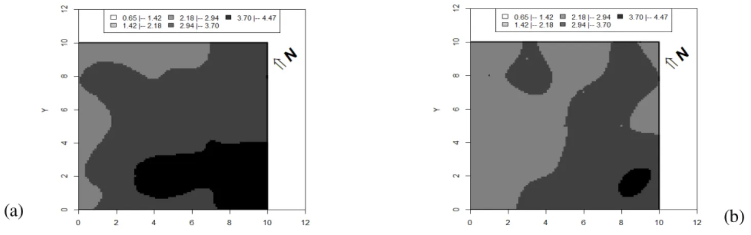
The Post-plot graphs (Figure 2) illustrate the average values of the irrigated water depth obtained in each of the 100 collectors for the non-compensating (Figure 2a) and co mpensating sprinklers (Figure 2b). For each type of sprinkler, a directional tendency (Figure 2) of the average irrigation water depth in the direction of 135º in the azimuth system (northwest-southeast) was observed. This directional trend was also confirmed for the sprinkler types, due to the existence of a significant linear association, at 5% probability, between the values of the average irrigation water depth, with the coordinates of the X and Y axes of the area, estimated by the Pearson linear coefficient (Table 3).
This can be explained, because according to Souza et al. (2013) the dominant direction of the winds in the region of Cascavel/PR is northwest-southeast (NE).
Shull & Dy lla (1976), observing the effects of wind speed on the water distribution in a high pressure sprinkler, concluded that increasing wind speed increased
the jet’s wind direction, shortened it and narrowed the
range in the normal d irection to the direction of the wind, causing a decrease in wet diameter.
In addition, it was observed for ACS that the discrepant points correspond to the highest average depth values and are located in the southeast region of the study area (Figure 2b).
TABLE 3. Pearson’s linear correlation coefficient of the average irrigation water depth (mm) with compensating (ACS) and non-compensating sprinklers (A NCS), with the geographical coordinates of the axis -X and the axis-Y.
Pearson’s linear correlation ANCS ACS
Axis-X 0.5786* 0.5623*
Axis-Y -0.6889* -0.3693*
*: indicates significant linear correlation (p-value <0.05) at 5% probability.
FIGURE 2. Post-plot Graphic of the average irrigation water depth (mm) with non-compensating (a) and (b) compensating sprinklers. Circu lated points represent discrepant values in the one-dimensional analysis.
As the presence of the directional tendency influences the assumption of stationarity of the stochastic process in the geostatistical modeling, this was incorporated to the study of spatial dependence of the average irrigation water depth, considering that the mean of the stochastic process is explained by means of a linear regression model, where the coordinates of the X and Y axes are the covariates (Santos et al., 2011; Monego et al., 2015).
The estimated values for the spatial linear model that describes the spatial dependence structure of the average irrigation water depth using these sprinkler systems are presented in Table 4. The best predicted model for the covariance function was the Gaussian (with nugget effect 1 1+ 2 =0.057 and practical range
a =13.81 m), when the compensating sprinkler was used, and the exponential model (with nugget effect
1 sill 1+ 2 =0.06 and practical range a
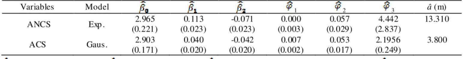
=3.8m), when the non-compensating sprinkler was used. The estimated values for relative nugget effect RN E = 100 1/( 1+ 2) indicated that there is a strong spatial dependence of the variable average water depth for the two types of sprinklers used ( (Cambardella et al., 1994). It can be observed that the variables average water depths obtained by the use of the two types of sprinklers presented similar estimates of nugget effect and contribution. However, they presented a significant difference in the estimated values of the practical range for the average irrigation water depth, being 3.80 m for the compensating sprinklers and 13.31 m fo r the non-compensating sprinklers. Thus, it is observed that the radius of spatial dependence for the average irrigation water depth is higher in the non-compensating sprinkler.
TABLE 4. Estimated values for the parameters of the geostatistical models of the average irrigation water depth (mm) wit h compensating (ACS) and non-compensating (ANCS) sprinklers. In parentheses the standard deviations of the estimates of the parameters of the geostatistical model.
Variables Model 1 2 3 â (m)
ANCS Exp . (0.221) 2.965 (0.023) 0.113 (0.023) -0.071 (0.003) 0.000 (0.029) 0.057 (2.837) 4.442 13.310
ACS Gaus. (0.171) 2.903 (0.020) 0.040 (0.020) -0.042 (0.002) 0.007 (0.017) 0.053 (0.249) 2.1956 3.800
1: estimated nugget effect; 2: estimated contribution; 3: estimation of an auxiliary parameter; â = g( 3): estimated practical
range ; and : estimates of linear regression adjusted to estimate the average water depth (mm) as a function of the x and y coordinates; Exp.: exponential; and Gaus.: Gaussian.
In Table 4 it can be observed that while the
compensating sprinklers
( as
non-compensating
( ,
there was a direct influence of the X coordinate and an inverse influence of the Y coordinate in relation to the estimated values for the average irrigation water depth (mm). That is, the larger the value of the X coordinate and the smaller the value of the Y coordinate, the larger the average water depth (mm). This confirms the directional tendency in the 135º direction following the azimuth system, shown in Figure 2. However, we observe a greater influence of the Y coordinate for A NCS.
With the estimated models (Table 4) of the spatial dependence structure of the average irrigation water depth (mm), for the non-compensating sprinkler systems
(exponential structure, = 0.05 ) and compensating (Gaussian structure, = 0.007
FIGURE 3. Map of the spatial variability of the average irrigation water depth (mm) by the non -compensating (a) and (b) compensating sprinklers.
In addition, for ANCS, estimated values ranged from 2.18 to 4.47 mm, whereas for ACS, values estimated in 98% of the area varied between 2.18 and 3.69 mm (Table 5) during the tests performed, which justifies the statistical difference of the irrigated med iu m depths between the two types of sprinklers (Table 2) and greater variability (CV = 11.70%) of the distribution for non-compensating sprinklers (Table 2).
TABLE 5. Percentages calculated by class for the average irrigation water depth (mm) of non -compensating and compensating sprinklers.
Variables 0.65 – 1.41 1.42 – 2.17 Classes of the average irrigation depth (mm) 2.18 – 2.93 2.94 – 3.69 3.70 – 4.47 Total
ANCS 0.00% 0.00% 18.79% 60.00% 21.21% 100%
ACS 0.00% 0.00% 50.87% 47.04% 2.09% 100%
The similarity measures (Table 6) for the comparison of the thematic maps (Figure 3) of the average irrigation water depth (ANCS and ACS) indicate low similarity (De Bastiani et al., 2012) between the maps using the two types of sprinklers (GA^ 0.85, 0.67
^
K and
67 . 0 ^
T ). Thus, it is possible to deduce that there are differences in water depth between the two types of sprinklers, and that the compensating sprinklers presented better uniformity of water distribution, as already identified by Tamagi et al. (2016) by means of the uniformity coefficients (CUC, CUD and CUE).
TABLE 6. Estimated values of similarity measures between the average irrigation water depth (mm) maps of non-compensating sprinkler irrigation (ANCS) and compensating sprinkler (ACS).
Pair of Variables for comparison
Similarity Indexes Global Accuracy
( ) Kappa ( ) Tau ( ) ANCS – ACS 0.4568 0.1206 0.3210
CONCLUS IONS
Regarding the spatial dependence structure described by the estimated geostatistical models, there was a greater spatial dependence radius between the values of the average irrigation water depth when the non-compensating sprinkler was used.
The dominant direction of the winds in the region of Cascavel/PR, wh ich is northwest-southeast (NE), and the wind speed, which on average was above 2 m s-1 during the execution of the tests, the existence of a
directional tendency (north-south-east direction) of the mean irrigation water depth values applied for both compensating and non-compensating sprinklers. This can only be observed with the construction of maps of spatial variability of the applied water depths, which would not be possible, using only uniformity coefficients, which demonstrates the importance of using several tools for data analysis in the irrigation systems.
The compensating sprinklers applied a s maller amount of water (averaging 13.1%), with a greater spatial distribution of water (CV = 9.72%) than non-compensating sprinklers (CV = 11.70%). Th is is most evident by the low similarity obtained between the maps of spatial variab ility, considering that for the compensating sprinklers 98% of the area had a depth varying between 2.18 and 3.69 mm, whereas for non-compensating sprinklers only 78.8% of the area received this water depth.
It is concluded, therefore, the use of compensating sprinklers bring better results as the distribution of water depth in sprinkler irrigation systems.
ACKNOWLEDGMENTS
The authors would like to thank the CNPq, CAPES and the Araucária Foundation for the support to the development of this research.
REFERENCES
ANA - Agência Nacional de Águas (2017) Atlas Irrigação: uso da água na agricultura irrigada. Brasília, ANA. 86p.
Alves AD, Castro PT (1995) Desempenho de um sistema de irrigação por aspersão tipo canhão hidráulico sob diferentes condições de velocidade de vento na região de Paracuru, CE. Engenharia Rural 6(2):79-84.
ABNT - Associação Brasileira de Normas Técnicas (2000) Equipamentos de irrigação agrícola – Aspersores rotativos. Parte 2: Uniformidade de distribuição e métodos de ensaio NBR ISSO 7749 – 2. Rio de Janeiro, 6p.
Bernardo S (2006) Manual de irrigação. Viçosa, UFV, 8ed. 625p.
De Bastiani F, Uribe-Opazo MA, Dalposso GH (2012) Co mparison of maps of spatial variability of soil res istance to penetration constructed with and without covariables using a spatial linear model. Rev ista Engenharia Agríco la 32(2):394-404. DOI: http://d x.doi.o rg/10.1590/S0100-69162012000200019.
De Bastiani F, Cysneiros AHMD, Uribe-Opazo MA, Galea M (2015) Influence diagnostics in elliptical spatial linear models. Test 24(2):322–340. DOI:
http://dx.doi.org/10.1007/s11749-014-0409-z.
Cambardella CA, Moorman TB, Novak JM, Parkin TB, Karlen DL, Turco RF, Konopka AE (1994) Field scale variability of soil properties in Central Iowa soils. Soil Science Society of A merica Journal 58:1501-1511. DOI: http://dx.doi.org/10.2136/sssaj1994.036159950058000500 33x.
Costa SC, Castro PT (1993) Desempenho de um Sistema de irrigação autopropelido sob diferentes condições de velocidade de vento. Engenharia Rural 4:102-116. Cressie N (2015) Statistics for Spatial Data. New York: John Wiley. 928p.
Faraco MA, Uribe-Opazo MA, Silva EAA, Johann JA, Borssoi JA (2008) Selection criteria of spatial variability models used in thematical maps of soil physical attributes and soybean yield. Revista Brasileira de Ciência do Solo 32(2):463-476. DOI: http://d x.doi.o rg/10.1590/S0100-06832008000200001
Faria LC, Beskow S, Colo mbo A, Oliveira HFE (2012) Modelagem dos efeitos do vento na uniformidade da irrigação por aspersão: aspersores de tamanho méd io. Revista Brasileira de Engenharia Agrícola e A mbiental 16(2):133-141. DOI: http://d x.doi.o rg/10.1590/S1415-43662012000200002
Fravet AMM, Cruz RL (2007) Qualidade da água utilizada para irrigação de hortaliças na região de Botucatu-SP. Irriga 12(2):144-155.
Frizzone JA, Rezende R, Freitas PSL (2011) Irrigação por aspersão v. 1. Maringa, Eduem. 271p.
Go mes FP (2000) Curso de estatística experimental. Piracicaba, Degaspari, 14ed. 477p.
Grego CR, Coelho RM, Vieira SR (2011) Critérios morfológicos e taxonômicos de latossolo e nitossolo validados por propriedades físicas mensuráveis analisadas em parte pela geoestatística. Revista Brasileira de Ciência do Solo 35(2):337-350. DOI:
http://dx.doi.org/10.1590/S0100-06832011000200005
Guedes LPC, Uribe-Opazo MA, Ribeiro JR PJ (2013) Influence of incorporating geometric anisotropy on the construction of thematic maps of simu lated data and chemical attributes of soil. Chilean Journal of Agricultural Research 73(4):414-423. DOI:
http://dx.doi.org/10.4067/S0718-58392013000400013 Justi AL, Vilas Boas MA, Sampaio SC (2010) Índice de capacidade do processo na avaliação da irrigação por aspersão. Engenharia Agrícola 30(2):264-270. DOI: http://dx.doi.org/10.1590/S0100-69162010000200008 Lu A, Wang X, Qin X, Wang K, Han P, Zhang S (2012) Multivariate and geostatistical analyses of the spatial distribution and origin of heavy metals in the agricultural soils in Shunyi, Beijing. Science of the Total Env iron ment 425:66-74. DOI:
http://dx.doi.org/10.1016/j.scitotenv.2012.03.003 Martins JFS, Cunha US, Neves MB, Mackedanz V, Vinhas MR, Mattos MLT, Afonso APS (2008) Influência de períodos de supressão da irrigação por inundação da cultura do arroz (Ory za sativa) na população do gorgulho aquático Oryzophagus oryzae (Costa Lima) (Co leoptera: Curculionidae) e produção de grãos. In: Congresso Brasileiro de Entomo logia. Uberlândia, Universidade Federal de Uberlândia. Resumos...
Monego MD, Ribeiro JR PJ, Ramos, P (2015) Co mparing the performance of geostatistical models with additional information fro m covariates for sewage plu me
characterization. Environ mental Science and Po llution Research 22(8):5850-5863. DOI:
http://dx.doi.org/10.1007/s11356-014-3709-7
Nogueira LC, Souza F (1987) Avaliação de dois sistemas de irrigação por aspersão. II – Análise da uniformidade de distribuição. In: Congresso Brasileiro de Engenharia Agrícola. Jundiaí, Anais...
Oliveira GA , Araújo WF, Cru z PLM, Silva W LM, Ferreira GB (2011) Resposta do feijão-caupi as lâminas de
irrigação e as doses de fósforo no cerrado de Roraima. Revista Ciência Agronô mica 42(4):872-882.
Oliveira FE de, Colo mbo A, Faria LC, Prado GDO (2012) Efeitos da velocidade e da direção do vento na
uniformidade de aplicação de água de sistemas
autopropelidos. Revista Engenharia Agrícola 32(4):669-678. DOI: http://d
x.doi.org/10.1590/S0100-69162012000400006
Oliver MA, Webster RA (2014) A Tutorial guide to geostatistics: computing and modelling variograms and kriging. Catena 113:56-69. DOI:
https://doi.org/10.1016/j.catena.2013.09.006
Robinson DP, Lloyd CD, Mckinley JM (2013) Increasing the accuracy of nitrogen dioxide (NO2) pollution mapping using geographically weighted regression (GW R) and geostatistics. International Journal of Applied Earth and Geoinformation 21(1):374-383.DOI:
https://doi.org/10.1016/j.jag.2011.11.001
Rocha FA, Pereira GM, Rocha FS, Silva JO (2005) Análise da uniformidade de distribuição de água de um equipamento autopropelido. Irriga 10(1):96-106.
Santos GR, Oliveira MS, Lou zada JM, Santos AMRT (2011) Krigagem simples versus krigagem universal: qual o preditor é mais preciso? Energ ia na Agricu ltura
26(2):49-55. DOI:
http://dx.doi.org/10.17224/EnergAgric.2011v 26n 2p49-55
Schemmer, RC, Uribe-Opazo, MA, Galea, M, Assumpçâo, RAB (2017) Spatial Variability of soybean yield through a reparameterized t-student model. Revista Engenharia Agrícola 37(4):760-770. DOI:
http://dx.doi.org/10.1590/1809-4430/EnergAgric.v.37n 4p760-770/2017
Shull H, Dy lla AS (1976) Traveling boom sprinkler operation in Wind. Transactions of the ASAE 19(3):501-504.
Souza AP, Pereira JBA, Silva LDB, Guerra JGM, Carvalho DF (2011) Evapotranspiração, coeficientes de cultivo e eficiência do uso da água da cultura do pimentão em diferentes sistemas de cultivo. Acta Scientiaru m Agronomy 33(1):15-22. DOI:
http://dx.doi.org/10.4025/actasciagron.v33i1.5527 Souza R.C.M. de, Uribe-Opazo MA, Hosokawa RT, Johann, JA, Guedes LP (2013) Influence of the eucalyptus windbreaks aerodynamic system on the soybean crop in West of Parana, Brazil. Journal of Food, Agriculture & Environment 11(2): 930-935. Available in:
https://www.wflpublisher.com/Abstract/4472.
Tamag i JT, Uribe-Opazo MA, Johann JA, Vilas Boas MA (2016) Uniformidade de distribuição de água de irrigação por aspersores compensantes e não compensantes em diferentes alturas. Irriga 21(4):631-647. DOI:
http://dx.doi.org/10.15809/irriga.2016v21n4p 631-647 Uribe-Opazo MA, Borssoi JA, Galea M (2012) Influence diagnostics in Gaussian spatial linear models. Journal of Applied. Statistics 39(3):615-630. DOI: