Renato Santos Aranha
A method to estimate the Macroscopic
Fundamental Diagram using Bus GPS Data
Rio de Janeiro, Brazil
2019
Renato Santos Aranha
A method to estimate the Macroscopic Fundamental
Diagram using Bus GPS Data
Master Thesis presented to the School of Ap-plied Mathematics as partial requirement to obtain the Masters Degree in Mathematical Modeling
Fundação Getulio Vargas - FGV Escola de Matemática Aplicada - EMAp
Programa de Pós-Graduação em Modelagem Matemática
Supervisor: Dr. Eduardo Fonseca Mendes
Co-supervisor: Dr. Renato Rocha Souza
Rio de Janeiro, Brazil
2019
Dados Internacionais de Catalogação na Publicação (CIP) Ficha catalográfica elaborada pelo Sistema de Bibliotecas/FGV
Aranha, Renato Santos
A method to estimate the Macroscopic Fundamental Diagram using bus GPS data / Renato Santos Aranha. – 2019.
63 f.
Dissertação (mestrado) -Fundação Getulio Vargas, Escola de Matemática Aplicada.
Orientador: Eduardo Fonseca Mendes. Coorientador: Renato Rocha Souza. Inclui bibliografia.
1. Engenharia de tráfego – Modelos matemáticos. 2. Trânsito – Fluxo – Modelos matemáticos. 3. Tráfego urbano – Modelos matemáticos. I.Mendes, Eduardo Fonseca .II. Souza, Renato Rocha. III. Fundação Getulio Vargas. Escola de Matemática Aplicada. IV. Título.
CDD – 388.4131
Acknowledgements
To the friends I have made along the master journey, I am thankful for the company and good discussions throughout the coursework. Whether through sharing ideas and conversations that have led us to conclude endless lists of exercises, going to coffee breaks together or just by relaxing conversation, know that daily living was very important for me to take up the routine of studies that I have been away for some years, because of my job. João Marcos "Ralado", Lucas Meireles, Antônio Sombra, Lucas Farias "IMPA", Gabriel Jardim, Fernando, Thiago Trabach, Otto and Bruno Lucian, thank you!
To friends I have made working for more than 7 years at B2W: Eduardo Dabul, Gerson, André Beiler, Bruno Cunha, Wiliam, Dan, Gustavo Melo, Plinio, Allan, Paolo Ghiu, Bruno Goulart, Eric, Rodrigo Rangel, Sel, Álvaro and Rodrigo Póvoa, and to great friends of life: Rafael Massa, Kayo Araujo, Fabricio Rabello, Rodrigo "Bravo", Alexandre Sardinha and Marcio Taddei.
To my mom, Kátia Regina, who always gave me love, encouraged and supported me in all the choices I have made in my life, and to my father, José Renato, a professor of physics who, with his interest in science, was a reference in my choice for Physics at undergrad.
To my sister-in-law Thais, to Pedro, and to my mother-in-law Nely, for the family living, support and moments of relaxation.
To professors Hugo de la Cruz and Paulo Cesar, for the very good classes taught in Computational Simulation and Probability courses.
To my supervisors, Eduardo Mendes (Duda) and Renato Souza, for agreeing to guide me in the thesis, for believing in my work and also for giving me a research grant to work on the web price index project (IPC-W). Duda, in addition to the enlightening discussions on the dissertation, thank you for so many conversations and tips on time organization, Statistics, Machine Learning, scientific writing and research planning.
Finally, I especially thank my wife, Tatiana, for her constant support in all aspects of life, for encouraging the difficult decision to dedicate myself exclusively to the master’s degree, for understanding when I needed to be absent to study, and for sharing life with me, giving me the opportunity to be by her side and enjoy her love and affection.
Now in Portuguese, my dear first language:
Aos amigos que fiz durante o mestrado, agradeço pela companhia e pelas discussões ao longo das disciplinas. Seja pelo compartilhamento de idéias e conversas que nos levaram a conclusão de infindáveis listas de exercícios, pelas idas em conjunto aos coffe breaks ou apenas pelos papos descontraídos, saibam que a convivência diária foi muito importante para que eu retomasse a rotina de estudos da qual eu já estava afastado há alguns anos, por estar no mercado de trabalho. João Marcos, Lucas Meireles, Antônio Sombra, Lucas Farias "IMPA", Gabriel Jardim, Fernando, Thiago Trabach, Otto e Bruno Lucian, obrigado!
Aos amigos que fiz ao longo de mais de 7 anos trabalhando na B2W: Eduardo Dabul, Gerson, André Beiler, Bruno Cunha, Wiliam, Dan, Gustavo Melo, Plinio, Allan, Paolo Ghiu, Bruno Goulart, Eric, Rodrigo Rangel, Sel, Álvaro e Rodrigo Póvoa, e aos meus grandes amigos de sempre: Rafael Massa, Kayo Araujo, Fabricio Rabello, Rodrigo "Bravo", Alexandre Sardinha e Marcio Taddei.
À minha mãe, Kátia Regina, que sempre me deu amor, me incentivou e deu suporte em todas as escolhas que fiz, e ao meu pai, José Renato, um professor de Física que, com seu interesse na ciência, foi uma referência na minha escolha por cursar Física na graduação.
À minha cunhada Thais, ao Pedro, e a minha sogra Nely, pela convivência, apoio e momentos de descontração.
Aos professores Hugo de la Cruz e Paulo Cesar, por ministrarem tão bem as disciplinas de Simulação Computacional e Probabilidade.
Aos meus orientadores, Eduardo Mendes (Duda) e Renato Souza, por aceitarem me orientar na dissertação, por acreditarem no meu trabalho e por me concederem uma bolsa de pesquisa para atuar no projeto de índice de preços web (IPC-W). Duda, além das discussões sobre a dissertação, obrigado pela muitas conversas e dicas sobre organização de tempo, Estatística, Machine Learning, escrita científica e planejamento de pesquisa.
Por fim, agradeço à minha esposa, Tatiana, pelo suporte constante em todos os aspectos da vida, por apoiar e incentivar a difícil decisão de me dedicar de forma exclusiva ao mestrado, por entender quando precisei ficar ausente para estudar, e por compartilhar a vida comigo, me dando a oportunidade de estar ao seu lado e desfrutar do seu amor e carinho em todos os momentos.
Abstract
Some approaches have been proposed by literature to describe the traffic state for a network, such as kinematic wave theory (using concepts from Physics), cell transmission models or macroscopic traffic simulation models. However, many of them have severe limitations regarding traffic state change or require a lot of computation time. For this reason, researchers have been examining for last years the existence of a simple and fast way that can sufficiently describe the dynamics of a road network. As a result, the concept of the Macroscopic Fundamental Diagram (MFD) - an object (empirical relation, theoretical model or both) that relates the average flow to the average density of a network, capturing so the essential network situation - was developed. Once the MFD of the network is known, all that is needed to have a traffic state estimation is to locate where the system is on the MFD at any desired moment, so it serves as a fundamental object for macroscopic traffic flow models. These family of models allow describing the spatio-temporal evolution of traffic density, for instance, and lead to clever solutions that optimize the existing traffic system. Thus, the objective of this project is to present a method for obtaining a network MFD using bus GPS data and a data structure developed by Uber (Uber’s H3 Hexagonal Hierarchical Spatial Index). We use a raw data collection of latitude and longitude data points of buses in Rio de Janeiro, Brazil, from January 2018 to December 2018. It is worth mentioning that the resulting MFD of the proposed method serves as a basis to support the development of public transportation management systems, which is able to make accurate traffic state predictions. The findings confirm the usefulness of bus GPS data and Uber H3 structure in finding a Macroscopic Fundamental Diagram, especially the Density-speed one, and future research directions are addressed.
Key-words: Macroscopic Fundamental Diagram. Traffic Theory. Traffic State. Probe
List of Figures
Figure 1 – Traffic Mass Conservation . . . 25
Figure 2 – Fundamental Diagrams. . . 27
Figure 3 – MFDs obtained by Daganzo and Geroliminis (2008) for San Francisco (a) and Yokohama (b) . . . 28
Figure 4 – H3 enables users to partition the globe into hexagons for more accurate analysis. H3 (2018) . . . 32
Figure 5 – Maps depicting the process of bucketing points with H3: cars in a city; cars in hexagons; and hexagons shaded by number of cars (density). H3 (2018) . . . 32
Figure 6 – Possible regular polygons that tesselate. The figure shows distances from a triangle to its neighbors, a square to its neighbor, and a hexagon to its neighbors. . . 33
Figure 7 – H3 Hexagons used to subdivide areas into smaller structures . . . 33
Figure 8 – Bus GPS points visualization using Folium . . . 35
Figure 9 – Raw data: JSON to DataFrame . . . 45
Figure 10 – Area selection and h3 partitioning. Image from github.com/uber/h3-py 47 Figure 11 – Example of networking partition: square selection - 665 bus line . . . . 48
Figure 12 – Example of networking partition: polygon selection - 665 bus line . . . 48
Figure 13 – Density-Speed relationship for a time window of 10 minutes and Hexagon sized 11 . . . 51
Figure 14 – Density-Speed relationship for a time window of 5 minutes and Hexagon sized 11 . . . 52
Figure 15 – Density-Speed relationship for a time window of 15 minutes and Hexagon size 12 . . . 52
Figure 16 – Speed-flow relationship for a time window of 10 minutes and Hexagon size 12 . . . 53
Figure 17 – Density-flow relationship for a time window of 10 minutes and Hexagon size 12 . . . 53
Figure 18 – Density-speed MFDs obtained by (DAGANZO; GEROLIMINIS, 2008) for San Francisco (a) and Yokohama (b) . . . 56
List of Tables
Table 1 – Table of Cell Areas for H3 Resolutions . . . 34
Table 2 – Estimated parameters and respective standard deviations for tested H3
hexagons resolutions and time aggregations . . . 54
List of abbreviations and acronyms
API Application Programming Interface
EU European Union
GPS Global Positioning System
ICT Information and Communication Technologies
LOS Level of Service
MFD Macroscopic Fundamental Diagram
MOE Measures of Effectiveness
OSM Open Street Map
Contents
I
Introduction
17
1 Introduction . . . 19
II Background and Literature Review
21
2 Background and Literature Review . . . 232.1 Fundamental Theory of Traffic . . . 23
2.2 Mass Conservation Law of Traffic . . . 24
2.3 Macroscopic Fundamental Diagram (MFD) . . . 26
2.4 Applications of MFD . . . 27
2.5 Influencing factors . . . 29
2.5.1 Road types . . . 29
2.5.2 Homogeneity of congestion . . . 30
2.5.3 Traffic light cycle . . . 31
2.6 H3: Uber’s Hexagonal Hierarchical Spatial Index . . . 31
2.6.1 Why hexagons? . . . 32
2.6.2 Why using H3? . . . 33
2.7 Folium and Leaflet for visualization . . . 34
III Methodology
37
3 Methodology . . . 393.1 Data Source: DATA.Rio . . . 39
3.2 Raw Data: Bus GPS . . . 40
3.3 Model setting . . . 42 3.3.1 Density . . . 43 3.3.2 Flow . . . 44 3.3.3 Mean speed . . . 44 3.4 Data Preparation . . . 45 3.4.1 Missing Data . . . 46 3.4.2 Map Matching . . . 46 3.5 Network partitioning . . . 47
IV Results
49
4 Results . . . 51 Discussion . . . 55 Conclusion . . . 59 4.1 Conclusion . . . 59 4.2 Future work . . . 59 Bibliography . . . 61Part I
Introduction
19
1 Introduction
As the share of urban population rises, the demand for urban mobility constantly increases, leading to traffic congestion issues, and understanding the basic traffic flow characteristics and techniques is an essential requirement for planning, design, and operation of any transportation system. In the past, this kind of problem was usually addressed with construction of new infrastructure, but this is neither advantage in terms of costs nor sustainable any more. Therefore, smart solutions that optimize the existing traffic system need to be studied and explored (for example, solutions can be found in the domain of smart cities control strategies that can contribute to improve the operation of road networks). Nevertheless, in order to establish a successful traffic control strategy, it is crucial to describe the traffic state accurately.
Following European Union (EU) oficial website (European(2019)), "a smart city is a place where the traditional networks and services are made more efficient through the use of data analysis, digital and telecommunication technologies, for the benefit of its inhabitants and businesses". A smart city goes beyond the use of information and communication technologies (ICT) for better resource usage, less emissions and other improvements. It also means smarter urban transport networks, upgraded water supply, waste disposal facilities, more efficient ways to light and heat buildings, more interactive and responsive city administration and safer public spaces.
Although recent, the concept of Smart City has already consolidated itself as a fundamental issue in the global discussion on urban development, and it drives, besides the technology solutions market, investment in high-level scientific research. Today, cities in emerging countries are investing billions of dollars in smart products and services to sustain economic growth and the demands of the population. Meanwhile, developed countries need to improve existing urban infrastructure to ensure the perpetuation of their economic status and the well-being and security of the population.
Assuming that urban environments and dynamics need to be interpreted as "indi-vidual systems" – with particularities and specific needs – and that it reacts according to the characteristics of their actors, we understand that smart cities will not be the same in all regions. That is, the technological solutions of one may not be applicable in another. Hence, the research problems that guides this study emerges: how bus traffic data of Rio de Janeiro can be used to infer general traffic states of the city?
The social contribution of this work consists in helping creating technical conditions for improvement in comfort and quality of life of the population through better urban management of traffic, based on data analysis. Besides that, in order to boost cities
20 Chapter 1. Introduction
development, it is necessary to have technology and projects designed to solve adversities of the present and to anticipate those of the future. This means more need of theoretical and experimental research that can help in the planning and efficient control of traffic.
In this context, we use probe data consisting of bus GPS data from Data Rio (the data and source are discussed in detail in chapter 3) for studying the dynamics of macroscopic traffic variables of the city of Rio de Janeiro, for the year of 2018. The aim is to propose a method for using bus GPS data to obtain traffic variables that enables the development of the Macroscopic Fundamental Diagram (MFD), an important object for estimating traffic state of a network or sub-network. In this way, urban network strategic planning to improve efficiency can be developed, based on a data-driven culture able to unveil insights into network behavior, well aligned with the Smart City concept.
Regarding the MFDs, the ones produced so far in the scientific literature have been based either on simulation data or on traffic data from the real world (this is our case), but finding a methodology to acquire the MFD that does not require large amounts of data is challenging. Instead of using granular traffic data, research efforts have been made to derive an analytical method to obtain the MFD, so that the need for large amounts of data is avoided, as exemplified by Geroliminis and Boyacı (2012). The goal of this approach type is to produce a general model that can be used to acquire the MFD. Still, network characteristics are affected by multiple and complicated variables, so the attempts to find a master model include trying to derive an estimation method with as few parameters as possible, so that methods produces, for example, an upper bound of the average flow in the network (if it complies with some regularity conditions, like homogeneous congestion levels).
This work is organized as follows:
Inchapter 1, it can be found the Introduction and context of what this research is about. Here, the research question and the objectives of this work should become clear. In
chapter 2, the Theoretical Reference of the research is presented in more detail. Still in this chapter, there is a Literature Review of Fundamental Theory of Traffic, Macroscopic Fundamental Diagram and relevant related topics.chapter 3 is dedicated to present the elements and frameworks used and the suggested Methodology, and chapter 4 brings a discussion about the Results obtained and potential future application and research directions.
Part II
23
2 Background and Literature Review
As mentioned in introduction, the main objective of this project is to propose a method for handling bus GPS data and estimate the Macroscopic Fundamental Diagram of an urban network. This chapter introduces the main theoretical concepts on which this work is based, and provides the associated reference. In this way, the necessary basis is contextualized for the correct understanding of the followed methodology and results obtained. The chapter begins with a discussion about Traffic Theory and then get into what is a Macroscopic Fundamental DiagramLeclercq, Chiabaut and Trinquier (2014). After that, a set of possible applications of the MFD is presented, supporting the idea that it is a reasonably simple and useful object either to support new traffic control strategies or to assess existing ones. The chapter ends presenting some factors that influence the success in constructing a well-defined MFD (well defined shape).
2.1
Fundamental Theory of Traffic
There are three basic approaches to traffic analysis: the macroscopic, which is concerned with describing the collective behavior of traffic flow, the microscopic, which is interested in the interaction between vehicles in a traffic stream, and the mesoscopic, whose units analyzed are groupings of vehicles that form in road systems.
Macroscopic analysis of traffic flow allows, for example, a design engineer to have a better understanding of the capacity limitations of the road systems and the evaluation of the consequences of occurrences that cause bottlenecks in them.
The microscopic analysis of the relations between vehicles on the same traffic chain allows studies of flow that are not necessarily homogeneous or uninterrupted. In general, the individualized treatment of vehicles requires more computational resources than the macroscopic approach.
The third one is the mesoscopic approach, in which the analysis consists of the study of vehicle groups in traffic streams (usually called platoons). An example of application derived from this method is the establishment of semaphore coordination policies. For many researches, the mesoscopic analysis does not really exists and its objects of study would be framed in the scope of macroscopic approach. For other authors, however, theoretical formulations about the behavior of vehicle groups are sufficient to make such a distinction.
The chosen approach of this thesis is the Macroscopic, where traffic analysis is based on the consideration that traffic streams are continuous media, and in order to study its behavior, the macroscopic approach makes use of some concepts from Physics,
24 Chapter 2. Background and Literature Review
particularly Hydrodynamics laws (Greenberg (1958) and Zhou J.(2016)), which is why the approach is also known as Hydrodynamic Analogy for Traffic.
Moreover, due to its characteristics and assumptions, the Macroscopic analysis successfully apply to the study of traffic with high density, but do not easily lend themselves to situations of rarefied traffic, where the behavior variation between drivers is greater. Another feature of Macroscopic theory is the requirement of the definition of three basic quantities (that will be presented in section 3.3), and as the characteristics of traffic vary in time and space, studies usually adopt average values (these averages can be temporal or spatial).
2.2
Mass Conservation Law of Traffic
In traffic modeling, in general, the equations (or systems of equations) are based on the physical principle of conservation. When physical quantities remain the same during some process, the conservation of these quantities occurs. Many elements in traffic dynamics are treated as conservative process (e.g. Kachroo (2008)), and interpreting this principle in a mathematical way makes it possible to predict the evolution of traffic density and velocity patterns over time.
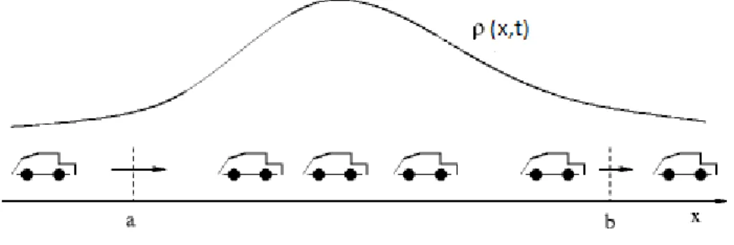
Let τ (x, t) be the density of vehicles (number of vehicles per unit of space) at the point x of space and t of time, and let f be the vehicular flux (number of vehicles per unit time). Now assume that f is a function of the density (flow function), that is, f = f (τ (x, t)). Defining this flow function f in a domain range [0, τmax], where τmax is the maximum
density of the network (this value is usually defined empirically, and can be interpreted as the maximum number of vehicles within the studied site). The number of vehicles in a segment between two points x1 and x2 at time t will be given by n =
Rx2
x1 τ (x, t)dx.
Assuming that vehicles do not "appear" or "disappear" within the studied segment, changes to the number of vehicles can only be caused by inflow or outflow at the boundaries, and as these boundaries flows are given by f (τ (x1, t)) and f (τ (x2, t)), the following expressions holds: dn dt = d dt Z x2 x1 τ (x, t)dx = f (τ (x1, t)) − f (τ (x2, t)) (2.1) d dt Z x2 x1 τ (x, t)dx ≈ τ (x, t)∆x (where ∆x = x2− x1) (2.2)
Combining the above relations and considering so that dndt ≈ ∂
2.2. Mass Conservation Law of Traffic 25 ∆x∂t∂τ (x, t), we obtain: ∂τ (x, t) ∂t = 1 ∆x dn dt = − f (τ (x2, t) − f (τ (x1, t)) ∆x ≈ − ∂f (τ (x, t)) ∂x (2.3)
Physically, the underlying concept can be interpreted as the principle of mass
conservation in vehicular traffic. For better understanding, consider a segment of a track,
as shown in Figure 1, with vehicles entering in the left side (point a) and exiting in the right side (point b). The variation in the number of vehicles in the ab segment will be defined by the difference between the number of incoming vehicles in a (given by f (τ (a, t))) and the number of vehicles exiting through b (given by f (τ (b, t))).
Finally, 2.3 can be written as:
∂τ (x, t) ∂t +
∂f (τ (x, t))
∂x = 0, (x, t) ∈ [(−∞, +∞), [0, +∞)] (2.4)
And the obtained equation (2.4) is defined as the basic law of conservation of vehicle density. Note that this equation is valid not only in the scope of traffic theory, but also in several areas of knowledge in Physics. This is an expression that represents, more generally, the law of conservation of a physical variable (in our case, this variable is the density τ (x, t)).
In addition, such a partial differential equation (PDE) is the main basis of the
LWR model, which was the first model used in the description of the traffic flow problem,
and is named after the works of Society (1955) and Richards (1956).
26 Chapter 2. Background and Literature Review
2.3
Macroscopic Fundamental Diagram (MFD)
The Macroscopic Fundamental Diagram describes the empirical relationship be-tween the three main measures of traffic flow theory, namely: volume or flow (q), density (k) and velocity (v), and was first proposed in byGreenshields et al. (1935) and later verified in several simulation and empirical studies. Within a FD, it is possible to observe three basic properties of traffic flow:
• The vehicle speed in traffic is inversely proportional to the number of vehicles (density) in the road;
• In free-traffic situations (the so-called free-flow regime), the volume of traffic increases with increasing density, while under congested flow regime, both the volume of traffic and speed decreases with increasing density;
• There is a critical phase transition point separating the free flow from the congested
flow regime.
One of the most important characteristics of Macroscopic Fundamental Diagram (MFD) is that it enables describing traffic at aggregated level. This means that MFD is a reasonably simple and useful object to support new traffic control strategies or to assess existing strategies. In a similar way that usual Fundamental Diagram (FD) relates the flow and the density at some street piece or road section, the MFD extends this concept at a larger urban network. More specifically, the MFD relates the number of vehicles in the network, which is frequently called accumulation, to the outflow from the network, which is usually expressed by the production (vehicles/hour), as well explained inMermygka (2016).
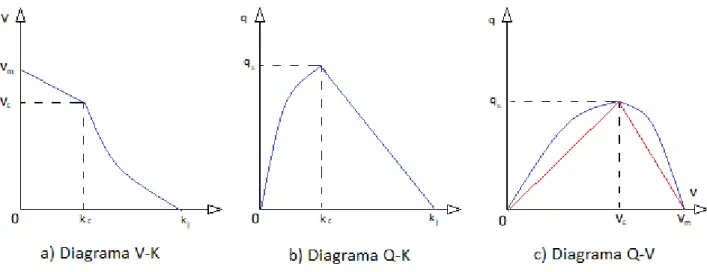
A sketch with typical examples of Fundamental Diagrams is shown in Figure 2. The possible diagrams consists of graphs that capture density-velocity (V-K-diagram), flow-density (Q-K diagram), and flow-velocity (Q-V diagram) relationships. Among these graphs, the Q-V diagram has special importance in this work, because it is observed in traffic engineering literature that this one is the most achievable when probe vehicle data – with some kind of bias – is available. Although the acquisition of traffic density data depends on specific collection methods, the speeds in tracks can be estimated by known methods, as can be seen in Wang and Xue (2014). To further describe a Q-V diagram, three values can be obtained: capacity(qc), critical speed (vc) and free traffic
velocity(vm).
The capacity qc represents the maximum volume of vehicles that a path holds
2.4. Applications of MFD 27
Figure 2 – Fundamental Diagrams.
To understand the direct and simple interpretation of Fundamental Diagrams, it should be noted that its possible graphs can change according to the probe data used and the physical characteristics of the network studied. Therefore, Fundamental Diagrams need to be obtained and calibrated according to the analyzed studied place, as pointed out in Gu et al. (2017).
As a concrete example, we can also refer toDaganzo and Geroliminis (2008), were the authors shows the existence of well defined instances of macroscopic fundamental diagrams for the velocity-density relationship (Figure 3), based on empirical data from the cities of San Francisco (USA) and Yokohama (Japan). The study was carried on city sites where any street with blocks of diverse widths and lengths – but no turns – were considered (their database context has intersections controlled by arbitrarily timed traffic signals).
2.4
Applications of MFD
The MFD has a variety of applications aiming to improve mobility in urban networks. It can be used as a useful tool for traffic managers to monitor their systems and assess the operating level of a network. It can also be used to provide necessary information for traffic control and state prediction. Keyvan-Ekbatani M. and Papageorgiou (2012) state that although MFD research is still active, the level of knowledge already achieved allows good and reliable base for traffic control strategies.
In Daganzo and Geroliminis (2008), the outflow rate obtained by the MFD is
proposed to be used as a way to evaluate the city’s accessibility and determine how it can be improved. If a new control strategy is implemented or an infrastructure change occurs, the MFD will most probably change its format, showing whether the measure was
28 Chapter 2. Background and Literature Review
Figure 3 – MFDs obtained byDaganzo and Geroliminis(2008) for San Francisco (a) and Yokohama (b)
successful. It is worth mentioning that area size of evaluation of traffic measurements is a very important topic. The reason is that an observed effect on a narrow area can be just a false result due to this narrow area considered. For instance, the implementation of a new traffic control algorithm at one intersection could improve the flow at this intersection, but maybe that is only because drivers now choose another intersection to go. This false assessment can be avoided by examining results provided by the MFD of a larger area.
Another example of application of the MFD is indicated inGeroliminis and Levinson (2009), where researchers describe the modeling of recurring congestion in a network in order to support pricing strategy. Their research uses MFD to develop a network-based
2.5. Influencing factors 29
congestion pricing scheme, and it was tested in the same place studied in Daganzo and
Geroliminis (2008) (Yokohama, Japan) for the morning peak congestion period. Their
results showed that the toll-case works very well compared to the no-toll case. With the application of an optimal toll price – based on Pigou (1920), Vickrey (1963) and Beckmann (1965) studies – delays were drastically reduced and the duration of the peak hour decreased. Simoni M. D. and Hoogendoorn (2015) also proposed a methodology to derive cost congestion pricing based on the network fundamental diagram, suggesting that a policy of time-dependent toll prices can be achieved using MFDs grouped by time periods. They tested their methodology in a simulated case study of the city of Zurich and found that this approach is more realistic than other methods that are usually applied to support tolling schemes.
Lastly, there is also one of the main performance indicators to assess traffic opera-tions: the Level of Service (LOS). It is represented by means of a grading system using one of the first six letters of alphabet (A – F), where A level denotes the best operating condition and F level denotes the worst one. The LOS scheme is based on road and network characteristics such as mean speed, critical density, drivers perceptions and others, and among traffic engineers, LOS is part of a group of representative statistics usually called Measures of Effectiveness (MOE).
To conclude, it has become clear that there is a variety of studies investigating the advantages of applying MFD to support new traffic control strategies, or even assessing existing ones. These findings give support to the allegation that although MFD is a simple structure, it can be useful and powerful. This characteristic is the strongest reason that motivates its research.
2.5
Influencing factors
Factors that have impact on MFD shape have been the topic of interest of many research publications. The usual findings (Daganzo and Geroliminis (2008), Buisson and
Ladier (2009), Geroliminis and Sun (2011), Laval and Castrillón (2015)) suggest that
the main parameters that influence the MFD are: homogeneity levels of congestion, road types of the network, location of the loop detectors (not applicable in this thesis) and the characteristics of traffic lights (e.g. distance between them and time cycle). Except for loop detectors, these factors and its possible effects on the estimation of the MFD will be described in this section.
2.5.1
Road types
Traffic variables on freeways and urban roads are different. The traffic speed on freeways is usually higher than that on urban roads due to different speed limits, and
30 Chapter 2. Background and Literature Review
vehicles can usually travel more smoothly on freeways. This examples summarize what many research papers state: in order to derive MFD, the general recommendation is to divide the city into zones grouping geographic characteristics and road types. Within zones with the same road type, the recommendation is usually in the sense of separating signalized and non-signalized roads to avoid much scatter in the MFD. InGeroliminis and Sun (2011), for instance, it is concluded that MFD normally does not hold for freeway networks due to their different characteristics such as the absence of traffic signals and speed levels. On the other hand,Cassidy M. and Daganzo (2011) suggested that the MFD can be obtained in freeways, if some premises are considered.
These few examples shows how road types is an important topic to consider in evaluating and interpreting the MFD shape.
2.5.2
Homogeneity of congestion
When studying factors that could influence the shape of MFD, one of the most cited in the literature – due to controversy – is the homogeneity of congestion over the network.
Daganzo and Geroliminis(2008) state that "universal MFDs should not be expected" in
case that congestion state is not consistent across the network studied, and there are some studies, likeBuisson and Ladier (2009) and Ji Y. and Qian (2010), indicating that homogeneity at congestion is indeed a necessary condition to obtain a well-defined MFD, and in the absence of this requisite, noise, scattering and false hysteresis effect should be found.
Therefore, although a bit unrealistic, the general conclusion is that the network need to have similar traffic state in all of its links in order to have an associated MFD. As this is a quite restrictive assumption, research has been developed to explore in more depth the homogeneity assumption, and Geroliminis and Sun(2011) used real traffic data from Yokohama (Japan) and Minnesota (USA) to empirically show that homogeneity traffic states in entire network is not absolutely necessary to achieve a MFD, and as long as the spatial distribution of congestion is similar for consecutive time intervals that have the same average network occupancy, the MFD is obtainable.
What this means is that they got to find a way to relax the homogeneity need, but now suggesting that spatial variability of density should be smooth and similar for time periods in which average network occupancy is about the same. Following this research finding,Ji and Geroliminis (2012) andKnoop V. L. and Hoogendoorn (2015) studied a method to divide the network in homogeneous zones with low variation in density.
2.6. H3: Uber’s Hexagonal Hierarchical Spatial Index 31
2.5.3
Traffic light cycle
Regarding traffic light cycle,Laval and Castrillón (2015) and Jong D. and
Hoogen-doorn (2013) investigated the effects of signal timing on the MFD. What they found
is that the cycle time of traffic light and their coordination between intersections are important issues to consider as influence in the underlying network MFD. One of the main conclusions from the papers is that when the signals settings change, then the shape and data variance of the MFD also changes.
2.6
H3: Uber’s Hexagonal Hierarchical Spatial Index
In order to obtain the aggregated traffic variables, Uber’s H3 framework is used H3 (2018). The framework consists in a discrete global grid system (Sahr Denis White (2003)) critical to analyze large spatial data sets, partitioning areas of the Earth into identifiable grid cells (more precisely, it is a multi-precision hexagonal tiling of the sphere with hierarchical indexes). Uber developed H3 with the main goal of using the grid system for efficiently optimizing ride pricing and dispatch and for visualizing and exploring spatial data. H3 enabled Uber researchers to analyze geographic information to set dynamic prices and make other decisions on a city-wide level. H3 led Uber to make some choices such as using hexagonal hierarchical indexes. The grid hexagons can be visualized in
Figure 4, and a sketch of the density calculating process can be seen in Figure 5. The
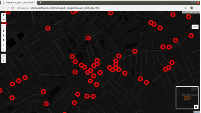
latter represents the usefulness of the framework for this thesis: Density K and Flow Q are calculated for every H3 hexagon of a choosen network piece, what this means is that the hexagons are the most granular network piece, so all the three variables presented are calculated for each hexagon in the network, and regarding framework, this is the main contribution of this thesis, and Figure 7 shows an example of our data being mapped by hexagons. The referred image is a mapping of a sample from 2018-01-01 data.
32 Chapter 2. Background and Literature Review
Figure 4 – H3 enables users to partition the globe into hexagons for more accurate analysis.H3(2018)
H3 was open sourced by Uber on Github earlier in 2018, giving access to a powerful solution, including Python bindings, as can be seen at github.com/uber/h3-py (by March 2019).
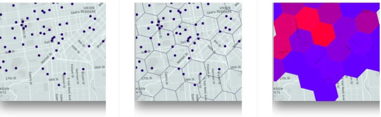
Figure 5 – Maps depicting the process of bucketing points with H3: cars in a city; cars in hexagons; and hexagons shaded by number of cars (density).H3(2018)
2.6.1
Why hexagons?
Among the possible three regular polygons that can tesselate an area (triangles, squares and hexagons), hexagons present the most suitable because there are only six direct neighbors (versus eight in squares and twelve in triangles), and the distance from the center of a reference hexagon to the center of its direct neighbours is constant. This provides computational advantage in calculations of dynamic phenomena like traffic flow, where vehicles are constantly moving and crossing the polygon boundaries. The geometrical view is shown in figure 6.
2.6. H3: Uber’s Hexagonal Hierarchical Spatial Index 33
Figure 6 – Possible regular polygons that tesselate. The figure shows distances from a triangle to its neighbors, a square to its neighbor, and a hexagon to its neighbors.
2.6.2
Why using H3?
The main advantage of using H3 in this thesis can be explained by the fact that gathering information and insights from our geospatial data requires analyzing data across entire city or parts of the city, and because cities are geographically diverse, this type of analysis needs to occur at a fine precision, and analysis at the finest granularity, considering the exact location where an event happens, is very difficult and expensive. Analysis on areas, such as neighborhoods within a city, is much more practical and viable. This eliminates the necessity of having detailed metadata about the streets, like length or number of lanes.
Figure 7 – H3 Hexagons used to subdivide areas into smaller structures
Another feature that Uber offers in its H3 solution is the possible of choosing hexagon size according to the usage. Table 1 shows the full resolution table available. There are 16 possible resolutions, and for this work, we have tested resolutions 11 and 12, because their suitable average hexagon area.
34 Chapter 2. Background and Literature Review
Table 1 – Table of Cell Areas for H3 Resolutions
2.7
Folium and Leaflet for visualization
Folium is a package that integrates the data wrangling strengths of the Python
ecosystem and the mapping strengths of the leaflet.js library. With it, it is very straight-forward to manipulate your data in Python, and then visualize it in on a Leaflet map
Folium(2013), as can be seen in Figure 8.
Leaflet is the leading open-source JavaScript library for mobile-friendly interactive maps. Weighing just about 38 KB of JS, it has many of the mapping features most geo-developers needAgafonkin (2017), and works efficiently across all major desktop and mobile platforms, having and extended offer of plugins and an easy to use documented API.
2.7. Folium and Leaflet for visualization 35
Part III
Methodology
39
3 Methodology
This chapter describes the framework used in this work, presents the concepts and data in detail, and shows the proposed methodology to produce the MFD. The most basic requirement is to have sufficient traffic data to estimate the traffic variables of density and
flow. As mentioned in section 2.3, for the majority of traffic theory research, the following terms are used to refer to these two variables: Density K: the number of vehicles in a space (unit e.g.: vehicles/km) and Flow Q: number of vehicles per unit time in the network (unit e.g.: vehicles/hour).
Due to experimental difficulties to collect the data necessary to analyze the complex traffic dynamics of urban networks, the majority of the literature uses simulation to obtain and explore synthetic MFDs. Despite this, the present work uses real data from a bus GPS database to propose a method to estimate MFD using a framework developed by Uber. This database is presented and detailed in sections section 3.1 and section 3.2. In the model setting section section 3.3, the formulas to calculate the main traffic variables are presented, and section 3.4is about our approach in data preparation. Finally, section 2.6
and section 2.7present the main frameworks used to obtain the variables needed to obtain
the MFD.
The workflow of the work in this thesis consists in gathering and treating data (performing null value evaluation, map matching, data concatenation and outlier detection), development of a tool to select a region of study of the city (such that is possible to choose a sub-network no generate the corresponding MFD), data aggregation to obtain the macro variables flow, density and speed, and finally the plotting of variables to get MFD.
3.1
Data Source: DATA.Rio
In October of 2001, the website Armazém de Dados was launched by the Instituto
Pereira Passos (IPP) - an autarchy of the municipal government of Rio de Janeiro,
responsible for urban planning in the city - as part of a pioneering project in transparency and development of statistical data, maps, studies and research focused on the City of Rio de Janeiro. In 2017, the underlying Data Warehouse underwent a great redesign of graphics as well as content. Now called DATA.Rio, the portal brings together the most advanced in terms of technology, providing access to raw data, information and delivering interactive tools for the population (CityHall (2019)).
DATA.Rio integrates a new model concept of planning, integration, management
40 Chapter 3. Methodology
in 2014, with the creation of Sistema Municipal de Informações Urbanas (SIURB), the Municipal Urban Information System. Since then, SIURB has become an information channel between the different municipalities, fostering the integration between them for the improvement of the production of data and information about Rio de JaneiroCityHall (2019).
Concerning data made available, the portal provides databases about a vast quantity of services and categorizes the content in many topics like Culture, Healthy, Sports and Leisure, Turism and other. For the purpose of this work, the relevant information is about bus GPS data, and is contained in the Transport group.
3.2
Raw Data: Bus GPS
Among all the data provided by DATA.Rio, the database chosen for this work is the open base that contains data on real time location of buses in the city of Rio de Janeiro. This data is generated and made available in a time frame of seconds, across every day of the year, and is streamed by a GPS installed in each bus.
According to Intelligent Transportation Systems (Mashrur Chowdhury; Amy(2017)) and Traffic Engineering (Treiber (2013)) literature, this type of data belongs to a category known as Vehicle-based data, and has the following advantages: larger coverage than loop detectors and cameras (another frequent source of traffic data), no particular infrastructure is to be built along the network and data capture is not affected by weather. The only limitation is the possible low location precision for GPS data.
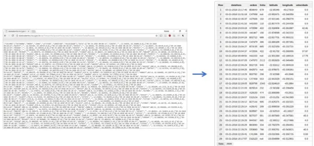
For this work, we use data of the year of 2018. This choice was made because, by the time of this thesis, this is the last full year available, and the total size of the 365 CSV files is around 150 Gigabytes. Each observation includes the position (latitude and longitude), the bus ID, the bus line ID and the datetime of the streamed signal, captured in time lapses between 1 and 10 minutes, so that we have approximately 3.000.000 measurements per day.
The disposal form is in JSON1, obtainable through <http://dadosabertos.rio.rj.gov. br/apiTransporte/apresentacao/rest/index.cfm/obterTodasPosicoes>. The information provided is the following:
• DATAHORA: Datetime of the signal issued by the GPS of the bus. • ORDEM : The bus ID. This ID is stamped on the side of the buses.
1 JSON (JavaScript Object Notation) is a lightweight data-interchange format. It is easy for humans to
3.2. Raw Data: Bus GPS 41
• LINHA: An ID equal to the bus line. Note that this is different from "ORDEM". A car with an "ORDEM" ID can have more than one "LINHA" ID, according to the studied day.
• LATITUDE: Latitude of the bus, at the moment of the GPS signal issued. • LONGITUDE: Longitude of the bus, at the moment of the GPS signal issued. • VELOCIDADE: Instantaneous velocity of the bus, at the moment of the GPS
signal issue.
It is worth to mention that the data available through the url is only of the current day. The full 2018 data was kindly made available by the School of Computing of the
42 Chapter 3. Methodology
3.3
Model setting
As already stated, in order to derive a network MFD, traffic variables (flow, density and speed) are needed, and the number of measured links of the network has to be as many as possible, so it can reflect the real network traffic state. In this subsection, the necessary mathematical concept for obtaining these macroscopic variables — i.e. variables describing the average behavior of the flow rather than of each individual vehicle — are presented.
When trajectory data are available, the generalized definitions ofEdie (1963) for traffic variables like density (k) and flow (q) are the basis for estimating the Macroscopic Fundamental Diagram (MFD). The expressions are, respectively:
k = P ti Ln∗ T = T T Ln∗ T (3.1) q = P di Ln∗ T = T D Ln∗ T (3.2) Where the summation is over the total number of vehicles within the studied period (e.g. trips in a 5 minutes window); ti and di are the travel time (e.g. seconds) and distance
(e.g. meters), respectively, for trip i during the analysis period; Ln and T are the total
network length (e.g. meters) and analysis period length (e.g. seconds), respectively. Note that equations3.1 and3.2only differ in the numerator: density k uses total time vehicles spend traveling within the studied network region during the analysis period (T T ) and
flow q uses total distance vehicles travel during the same period (T D).
In real-world applications, perfect T T and T D could only be known if detailed trajectories of all of the vehicles of the network are provided. However, in general it is very difficult to obtain such a complete database, and if these data are only provided for a subset of vehicles in the network (in our case, the bus GPS data), then equations3.1 and3.2 cannot be directly applied. In order to overcome this limitation,Nagle and Gayah (2014) proposed approximations, assuming that the fraction of vehicles serving as probes (ρ) can be estimated. These approximations are represented by the following equations:
ˆ k = P ti ρLn∗ T (3.3) ˆ q = P di ρLn∗ T (3.4) Where ti and di are, again, the travel time (e.g. seconds) and distance (e.g. meters),
respectively, for the probe vehicles (in our case, the buses). Regarding ρ, according to the traffic department of the state of Rio de Janeiro (Departamento de Trânsito do Estado do
3.3. Model setting 43
Rio de Janeiro, Detran-RJ) – an autarchy subordinated to the Government of the State of
Rio de Janeiro that is responsible for traffic inspection of vehicles and for issuing identity cards – the share of buses in the city, for 2018, is around 0.7%, as stated in detailed official statistics by Detran-RJ (2019).
Timing slice is a significant factor when aggregating traffic data. This decision has great influence in final results, especially for links with timed traffic signals. For example, vehicles have to queue in red light, resulting in high densities and zero flow on that section. When traffic lights turn green, the queue smoothly dissolves until vehicles pass the intersection without delay (approximately). Hence, the flow and speed will be higher, while the densities will be lower than those in the red light. So, it is reasonable to choose an aggregation period that is longer than the cycle time in order to reduce the influence of traffic lights. Aggregation time is usually set between 3 to 5 minutes (e.g. Mermygka (2016), Daganzo and Geroliminis (2008),Knoop V. L. and Hoogendoorn (2015)). In this
work, we test aggregation periods of 5, 10, and 15 minutes.
3.3.1
Density
The macroscopic characteristic called density of traffic is the number of vehicles present on a unit of road length at a given moment. Typically, it is expressed in veh/km and veh/m.
Note that the concept of density ignores the effects of traffic composition and vehicle lengths, and compared to Flow, determining the density is a bit more difficult. One possible method is using photography or video of the network site. From a photo of a road, for instance, the density is obtained by counting the number of vehicles present on a given road section of length X. In this case, Density is thus an instantaneous quantity that is valid for a certain time and region. Here, the Density is defined by the following practical equation:
k = m
X [number of vehicles / length unit] (3.5)
And considering a time–space region A, the expression can be written as:
k(A) =
P
n∈n(A)
tn(A)
|A| (3.6)
Where k(A) is the density in time–space region A; n(A) denotes the set of all the vehicles in A; tn(A) denote time spent.
44 Chapter 3. Methodology
3.3.2
Flow
The Traffic Flow is the number of vehicles passing a cross-section in a determined unit of time.
Whereas density is typically a spatial measurement, Flow is a temporal measurement. Sometimes other synonyms are used to define this variable, such as flux, throughput, current, or volume, but it typically depends on the researcher’s scientific background (e.g. physics, math, engineering).
The Flow can refer to a total cross-section of a road, or a part of it, and any unit of time may be used in obtaining Flow, such as 24h, one hour, 15 min, 5 min, etc. As mentioned insection 3.3, this thesis chooses to test time windows of the order of minutes. Apart from the unit of time, the time interval over which the Flow is determined is also important, but the two variables should not have diferent units. One can express the number of vehicles counted over 24h in the unit veh/second. The Flow (or flow) is a characteristic that is defined at a cross-section x for a period T, by:
q = n
T [number of vehicles / time unit] (3.7)
And considering a time–space region A, the expression can be written as:
q(A) =
P
n∈n(A)
dn(A)
|A| (3.8)
Where q(A) is the flow in time–space region A; n(A) denotes the set of all the vehicles in A; dn(A) denote distance traveled.
3.3.3
Mean speed
The third macroscopic variable to be considered is the mean speed of a traffic stream. It is usually expressed in kilometres per hour (or meters per second), and using an approach that considers direct measurements of individual vehicles speeds, we can generally obtain the mean speed as the total distance travelled by all the vehicles in the measurement region, divided by the total time spent by them in this region:
uL= N P 1=i Xi N P 1=i Ti (3.9)
In the above equation, Xi and Ti are the distance and time, travelled by the
3.4. Data Preparation 45
time–space region A, the expression can be written as:
u(A) = P n∈n(A) dn(A) P n∈n(A) tn(A) (3.10)
Where n(A) denotes the set of all the vehicles in A, and dn(A) and tn(A) denote
distance traveled and time spent.
3.4
Data Preparation
Considering that, for each network region or the whole network, there exists a relation between the three previously discussed macroscopic traffic variables (density K,
flow Q, and mean speed U, stated as:
Q = K ∗ U (3.11)
The most basic conclusion is that knowing two of them allows the calculation of the third one. This relation is often called the fundamental relation of traffic flow theory, and provides a close bond between the three involved quantities.
The data of each day were transformed from JSON to CSV (each CSV file rep-resenting one day), and then to Data Frames objects of Pandas2, as can be seen in
Figure 9:
Figure 9 – Raw data: JSON to DataFrame
2 Pandas is an open source, BSD-licensed library providing high-performance, easy-to-use data structures
46 Chapter 3. Methodology
3.4.1
Missing Data
As the GPS transmitting equipment of the buses are not properly working without fail all the time, it was found gaps in the data of some vehicles. Thus, it is necessary to be aware that not every trajectory of every bus is available for each of the observed days. But, fortunately, as there are data from a long period (2018), the available data is typically enough for this thesis purposes, and no data imputation needs to be considered.
3.4.2
Map Matching
Any measuring device, whether analog or digital, potentially displays results with a certain level of inaccuracy or noise. The inaccuracy of a GPS sensor system depends on the inaccuracy of the sensor itself, and also on factors such as landscape, movement speed of the device, the number of satellites involved and its location. In order to overcome this drawback, Map Matching method was applied.
Map Matching consists of taking a sequence of locations (e.g. latitude and longitude from GPS trajectory) and mapping them to the underlying closest road in network, considering the shortest euclidean distance to the nearby roads. The links were represented by one or more straight link segments, and each link segment was defined by a central point.
In terms of framework, a Python wrapper developed by Oderbolz (2014) for the OpenStreetMap API was used. OpenStreetMap (OSM) is a collaborative project to create a free editable map of the world, and rather than the map itself, the data generated by the project is considered its primary output.
3.5. Network partitioning 47
3.5
Network partitioning
I order to retrieve general characteristics of the city network, the entire network data is used to get an affordable MFD. But in practice there are to drawbacks in this approach: Computational cost and - most important - the non usefulness of the results for local traffic control strategy, and in the case that the networks are very large, network partitioning could be used to produce diferente MFDs for the parts that the network is divided. Taking this into account and using Shapely 3, we implemented an application
where the user can select an area of the city to study.
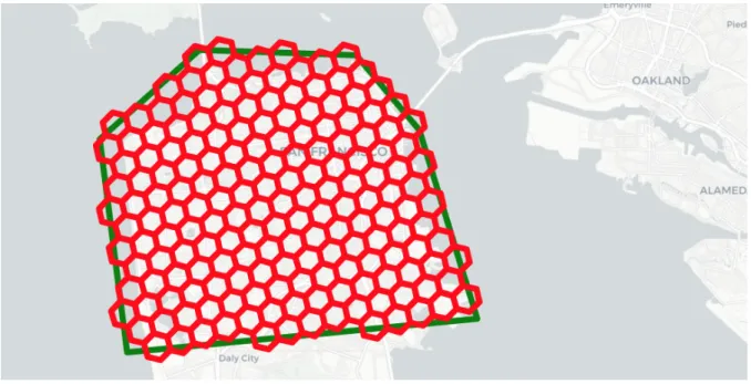
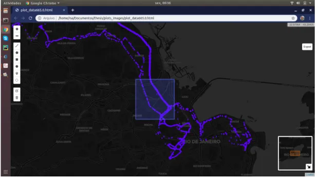
In Figure 10, there is an example of an area selection and the corresponding
partition with the hexagons of Uber H3. Figure 11andFigure 12 shows actual examples of our developed selection tool for 665 bus line, with square or polygon area selection. This feature provides the possibility of specific studies in places of interest.
Figure 10 – Area selection and h3 partitioning. Image fromgithub.com/uber/h3-py
48 Chapter 3. Methodology
Figure 11 – Example of networking partition: square selection - 665 bus line
Part IV
Results
51
4 Results
In this chapter, we set out the key experimental results obtained by the method proposed in this thesis. Using basic formulation, this thesis project proposed a method for estimating a Macroscopic Fundamental Diagram based on Bus GPS Data (a probe data of total traffic), and the result is very promising. The Density-speed relationship was the most well-defined one, as shown in Figure 13 (time window of 10 minutes and hexagon sized 11),Figure 14 (time window of 5 minutes and hexagon sized 11) and Figure 15(time window of 15 minutes and hexagon sized 12), where red lines shows confidence interval at 95%). The other relationship diagrams did not appeared so well defined, and possible reasons are discussed in chapter 4. Also, the described method is unique due to the usage of bus GPS data of Rio de Janeiro and H3 Uber’s Hexagonal Hierarchical Spatial Index. The figure below shows the relation between Speed and Density for a time window of 10 minutes and H3 hexagons structure with resolution 11 (see table 1 for reference).
52 Chapter 4. Results
The figure below shows the relation between Speed and Density for a time window of 10 minutes and H3 hexagons structure with resolution 11 (see table1 for reference).
Figure 14 – Density-Speed relationship for a time window of 5 minutes and Hexagon sized 11
The figure below shows the relation between Speed and Density for a time window of 15 minutes and H3 hexagons structure with resolution 12 (see table1 for reference).
53
The figure below shows the relation between Speed and Density for a time window of 10 minutes and H3 hexagons structure with resolution 12 (see table 1 for reference).
Figure 16 – Speed-flow relationship for a time window of 10 minutes and Hexagon size 12
The figure below shows the relation between Speed and Density for a time window of 10 minutes and H3 hexagons structure with resolution 12 (see table 1 for reference).
54 Chapter 4. Results
The Density-speed MFDs shows a high density of points for a narrow range (the so called mid-flow regime), and it was possible to fit a well shaped exponential relation, with a format very similar to the ones found by Daganzo and Geroliminis (2008). The parameters of our model, A ∗ exp−Bx+C are:
• A: a parameter that is more relevant for free flow regime (where density k is very low, near zero, leading the exponential to 1),
• B perhaps the most important one, as it defines the curvature of the function, and so is an indication of physical characteristics of the network studied: the more concave is the curve, more rapid is the network in relation to the change of traffic state, i.e. little changes in density indicates abrupt changes in velocity.
• C: location parameter of the model
Table 2 shows the estimated parameters and respective standard deviations:
Table 2 – Estimated parameters and respective standard deviations for tested H3 hexagons resolutions and time aggregations
55
Discussion
This chapter presents a discussion of the results presented in chapter 4. As shown there, the Density-speed relationships were the most well-defined ones (Figure 13,Figure 14
and Figure 15are examples), and although we have achieved these good results, the other
relationship diagrams did not appeared so well defined.
The diagrams showing Density-speed relationships shows a high density of points for a narrow range (the so called mid-flow regime). For this regions, we could fit a well shaped exponential relation, very similar in form to the ones found by Daganzo and Geroliminis (2008) for the cities of San Francisco and Yokohama, as can be seen in Figure 18, and the functional form of our model, A ∗ exp−Bx+C, is a good representation for this traffic regime. Regarding the parameters, A is a parameter that is more relevant for free flow regime (where density k is very low, near zero, leading the exponential to 1), C is just the location parameter of the model, and B is perhaps the most important one, as it defines the curvature of the function, and so is an indication of physical characteristics of the network studied: the more concave is the curve, more rapid is the network in relation to the change of traffic state, i.e. little changes in density indicates abrupt changes in velocity.
The application of the proposed estimation methodology of chapter 3 resulted in the MFDs here presented, however, although Density-Speed MFD appeared in a visible well shaped form, for regions of very low (the beginning of the graph) or high density (the tail), our data did not provided us with a comprehensible behaviour. These regions are associated with the traffic states of free flow and congested flow, indicating that with our data, apparently we are unable to capture these states. A similar finding was achieved
in Mermygka (2016). The resultant diagram did not appear to follow a pattern, showing
high variance and a great level of scattering, as can be seen in Figure 16 and Figure 17. The occurrence of all this scatter in the data, leads some traffic engineers to question the validity of the fundamental diagram, but as stated by the work from Kerner (2004), the fundamental diagram remains a fairly description of the average behaviour of a traffic stream, but it points that the key is to separate stationary periods from non-stationary ones. InTable 3, we show a list of known papers that tried to get a well shaped MFD either from simulation or real data. The colors in content of column Findings shows whether the paper had succeeded or not in finding a MFD: green means success, yellow means partial success and red means failing.
Besides that, other possible reasons are hypothesized, based on literature review: • Homogeneity of congestion. As discussed insubsection 2.5.2, some studies
56 Discussion
Figure 18 – Density-speed MFDs obtained by (DAGANZO; GEROLIMINIS,2008) for San Francisco (a) and Yokohama (b)
MFD, and in the absence of this requisite, noise and scattering can be found. • Biased data (only from buses). It could be reasonable because buses have a
stopping behavior (bus stops) and dedicated lanes.
• Penetration rate The penetration rate (ρ) of the buses is not so high (≈ 0.7%), and as this is a short percentage of city total traffic, the results may have suffered.
57 R efer enc e Data Network Findings Geroliminis and Daganzo ( 2008 ) Real Y ok ohama MFDs w ork in practice (go o d shap es) Daganzo and Geroliminis ( 2008 ) Real + Sim ula tion Y ok ohama, San F rancisco Shap es of MFD partially confirmed Buisson and Ladier ( 2009 ) Real USA (some cities) MFD m uc h scattered if detectors are no t ideally lo cated Ji Y. and Qian ( 2010 ) Sim ulation -Hybrid net w orks... (m uc h scattered MFD) Cassidy M. and Daganzo ( 2011 ) Real USA (some cities) MFD only holds if strea m is completely congested or in free flo w Mazloumian A. ( 2010 ) Sim ulation -Densit y-flo w v ery clear Geroliminis and Sun ( 2011 ) Real Y ok ohama Densit y-flo w v ery clear Kno op V. L. and Ho ogendo orn ( 2015 ) Sim ulation USA (some cities) Clear MFD Nagle and Ga y ah ( 2014 ) Sim ulation -MFD sho ws high h ysteresis lo ops
59
Conclusion
This last chapter present the conclusion and also recommendations of future work both for practical use and further research.
4.1
Conclusion
This thesis project successfully managed to use bus GPS to estimate traffic state (especially Density-Speed) with an MFD, and the study provides a good step towards empirical estimation of the Macroscopic Fundamental Diagrams using a type of data that is becoming increasingly abundant due to the high availability of devices that enables the use of GPS localization. The use of Uber H3 open source framework has proved useful, because it eliminates the necessity of having detailed metadata about the streets, like length or number of lanes.
The overall result is very significant because although MFDs have been proposed by the scientific community as a computationally efficient tool for modeling urban traffic networks and for the development of network-wide control strategies, in general it is difficult to obtain it (as exemplified in Table 3), and few experimental MFDs actually exists.
4.2
Future work
The subject should be further studied in order to obtain more plausible relationships (Density-Flow and Flow-Speed), but a simple process with low apparatus requirements was used to obtain the results, and in this way, a reliable foundation was created. So, as the results of this project are encouraging to further use the proposed method, possible directions are considered:
Pratical application:
• Evaluation of network changes: data driven input for network operational changes, such as new lanes or the impact of road closing for some kind of maintenance. In that case, as it is necessary to evaluate the effect of the change and assess the drawbacks that may occur, the MFD of the network helps because it may change due to the network alterations, so also the optimal capacity point will increase or decrease depending on the change.
60 Conclusion
• Support of policy-making decisions: In the case that a new government policy is being considered, information is needed on the effect of the policy on traffic. Frequently, the main outputs considered are improvements in the safety or the liveability of the city, but the impact on the traffic also needs to be taken into consideration, since it influences on life quality of population. So, the MFD can be used to provide information about whether the policy will have a positive or a negative impact on the traffic flow.
Further research:
• Application to other networks: a suggestion that could contribute to the potential generalization of the process is to apply this thesis method to the traffic state estimation of other urban networks. The application of the proposed process to other networks can also provide an indication on whether the MFD can be well defined in any urban network.
61
Bibliography
AGAFONKIN, V. an open-source JavaScript library for mobile-friendly interactive maps. 2017. <https://leafletjs.com/>. [Online; accessed 15-Mar-2019]. Cited on page: 34. BUISSON, C.; LADIER, C. Exploring the impact of homogeneity of traffic measurements on the existence of macroscopic fundamental diagrams. Transportation Research Record:
Journal of the Transportation Research Board, (2124):127–136, 2009. Cited 3 times on
pages 29, 30, and 57.
CASSIDY M., J. K.; DAGANZO, C. Macroscopic fundamental diagrams for freeway networks: theory and observation. Transportation Research Record: Journal of the
Transportation Research Board, (2260):8–15, 2011. Cited 2 times on pages 30and 57. CITYHALL. DATA.Rio. 2019. <http://www.data.rio/>. [Online; accessed 8-Jan-2019]. Cited 2 times on pages 39and 40.
DAGANZO, C. F.; GEROLIMINIS, N. An analytical approximation for the macroscopic fundamental diagram of urban traffic. Transportation Research Part B: Methodological,
42(9):771–781, 2008. Cited 10 times on pages 9, 27,28, 29, 30, 43,54, 55, 56, and57. DETRAN-RJ. Detran - Dados de veículos. 2019. <http://www.detran.rj.gov.br/
_estatisticas.veiculos/02.asp>. [Online; accessed 2-Mai-2019]. Cited on page: 43.
EDIE, L. C. Discussion of traffic stream measurements and definitions. 2nd International
Symposium on the Theory of Traffic Flow, 1963. Cited on page:42.
EUROPEAN, C. Cities using technological solutions to improve the
manage-ment and efficiency of the urban environmanage-ment. 2019. <https://ec.europa.eu/ info/eu-regional-and-urban-development/topics/cities-and-urban-development/
city-initiatives/smart-cities_en>. [Online; accessed 3-Jan-2019]. Cited on page: 19.
FOLIUM. Make beautiful, interactive maps with Python and Leaflet.js. 2013.
<https://python-visualization.github.io/folium>. [Online; accessed 15-Mar-2019]. Cited on page: 34.
GEROLIMINIS, N.; BOYACı, B. The effect of variability of urban systems
characteristics in the network capacity. Transportation Research Part B: Methodological,
46(10):1607–1623, 2012. Cited on page: 20.
GEROLIMINIS, N.; DAGANZO, C. Existence of urban-scale macroscopic fundamental diagrams: Some experimental findings. Transportation Research B, 2008. Cited on page: 57.
GEROLIMINIS, N.; LEVINSON, D. M. Cordon pricing consistent with the physics of overcrowding. Transportation and Traffic Theory 2009: Golden Jubilee, pages 219–240, Springer, 2009. Cited on page: 28.
GEROLIMINIS, N.; SUN, J. Properties of a well-defined macroscopic fundamental diagram for urban traffic. Transportation Research Part B: Methodological, 45(3):605–617, 2011. Cited 3 times on pages 29, 30, and 57.