How to deal with extreme observations in empirical finance: an application to capital markets

(1)

How to deal with Extreme Observations in Empirical Finance: An

Application to Capital Markets

Josué de Sousa e Silva

A Dissertation presented in partial fulfilment of the Requirements for the Degree of -Master in Finance

Supervisor:

Prof. Doutor José Dias Curto, Associate Professor, ISCTE Business School, Quantitative Methods Department

(2)

In the last few years, Extreme Value Theory (EVT) has gained increased importance in modeling extreme observations in all social sciences. This is especially true in finance, since EVT is a tool used to consider probabilities associated with extreme and rare events with catastrophic consequences, as happened in the Sub-prime crisis in 2007.

To model extreme observations, we use two different statistical distribution families in this thesis: Generalized Extreme Value (GEV) and Generalized Pareto Distribution (GPD). In this thesis, EVT methods were used to investigate and fit the empirical distribution of the monthly maximum and minimum return series of the FTSE 100, NIKKEI 225 and S&P500 indices to the theoretical GEV and GPD distributions. We have applied two approaches of extreme value theory, the Block Maxima and the Peaks Over Threshold (POT) approach, as well as the parametric approach of the Maximum Likelihood Estimate Method (MLE) for the distribution parameter estimation and the non-parametric approach of the Hill estimator. As a result of the application, we have seen that in the GEV distribution application, our data was well represented by the Fréchet and Weibull distributions. On the other hand, in the GPD distribution, using the parametric approach MLE, our data was mostly well represented by the Exponential and Beta distributions. However, applying the GPD using the non-parametric approach of the Hill estimator for the tail index, we have seen that the monthly maximum returns of our indices are well represented by the Pareto distribution.

JEL Classification: C13, C14.

Key Words: Extreme Value Theory, Generalized Extreme Value (GEV), Generalized Pareto Distribution (GPD), Stock Market Returns.

(3)

Nos últimos anos, a Teoria de Valores Extremos (TVE) tem ganho uma importância crescente no estudo de observações extremas em todas as ciências. Isto é especialemente verdade em finanças, uma vez que a TVE é uma ferramenta utilizada para analisar as probabilidades associadas a eventos extremos e raros com consequências catastróficas, como a crise do Sub-Prime em 2007.

Para modelar observações extremas, usamos duas famílias de distribuição estatísticas: Distribuição Generalizada de Valores Extremos (GEV) e a Distribuição Generalizada de Pareto (GPD).

Nesta tese, a TVE foi utilizada para investigar e ajustar a distribuição empírica dos retornos maximos e minimos mensais dos índices bolsistas FTSE 100, NIKKEI 225 e do S&P500 às ditribuições teóricas da GEV e GPD.

Aplicamos duas abordagens na aplicação da TVE, o método do Block Maxima e o método dos excessos de nível (POT), onde para a estimação dos parâmetros da distribuição recorremos ao método paramétrico da Máxima Verosimilhança, bem como ao método não-paramétrico através do estimador Hill.

Como resultado do estudo empírico na aplicação da GEV, verificamos que as séries são bem representadas pela distribuição de Fréchet e Weibull. Por outro lado, na aplicação da GPD, utilizando a abordagem paramétrica para o cálculo dos parâmetros da distribuição, as séries são bem representadas pelas distribuições exponencial e Beta. No entanto, a aplicação do GPD utilizando a abordagem não-paramétrica, verificou-se que a série dos retornos máximos mensais dos índices são bem representados pela distribuição de Pareto.

Classificação JEL: C13, C14.

Palavras-chave: Teoria de Valores Extremos, Distribuição Generalizada de Valores Extremos, Distribuição Generalizada de Pareto, Retornos de Mercados de Capitais.

(4)

I

List of Tables

Table 1:FTSE 100 Explanatory data analysis ... 20

Table 2:NIKKEI 225 Explanatory data analysis ... 20

Table 3:S&P 500 Explanatory data analysis ... 21

Table 4:LR Test and Log-Likelihood Results - GEV... 27

Table 5:FTSE 100 Maximum/Minimum Parameters - GEV... 28

Table 6:NIKKEI 225 Maximum/Minimum Parameters - GEV ... 30

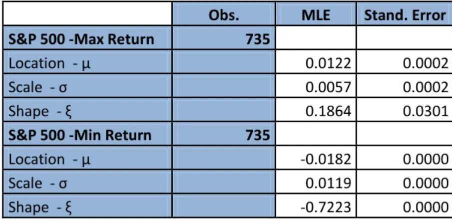
Table 7:S&P 500 Maximum/Minimum Parameters - GEV ... 32

Table 8:FTSE 100 LR Test and Log-Likelihood Results - GPD ... 35

Table 9:Maximum FTSE 100 Parameters - GPD ... 36

Table 10:Minimum FTSE 100 Parameters - GPD ... 37

Table 11:NIKKEI 225 LR Test and Log-Likelihood Results - GPD ... 38

Table 12:Maximum NIKKEI 225 Parameters - GPD ... 39

Table 13:Minimum NIKKEI 225 Parameters - GPD ... 40

Table 14:S&P 500 LR Test and Log-Likelihood Results - GPD ... 41

Table 15:Maximum S&P 500 Parameters - GPD ... 41

Table 16:Minimum S&P 500 Parameters - GPD ... 43

Table 17:FTSE 100 LR Test and Log-Likelihood Results – GPD (Hill Estimator) ... 46

Table 18:Maximum FTSE 100 Parameters - GPD (Hill Estimator) ... 46

Table 19:NIKKEI 225 LR Test and Log-Likelihood Results – GPD (Hill Estimator) ... 47

Table 20:Maximum NIKKEI 225 Parameters - GPD (Hill Estimator) ... 47

Table 21:S&P 500 LR Test and Log-Likelihood Results – GPD (Hill Estimator) ... 48

(6)

III

List of Figures

Figure 1:Asset returns distribution versus normal distribution 7

Figure 2:Block-maxima graph ... 9

Figure 3:Densities for the Fréchet, Weibull and Gumbel functions ... 11

Figure 4:Excesses over a threshold u graph. ... 12

Figure 5:Distribution Function and Distribution Over Threshold ... 12

Figure 6:Densities for the Beta, Pareto and Exponential functions ... 14

Figure 7:FTSE 100 Daily Returns Histogram ... 23

Figure 8:FTSE 100 Max Returns Histogram ... 23

Figure 9:FTSE 100 Min Returns Histogram ... 23

Figure 10:NIKKEI 225 Daily Returns Histogram ... 23

Figure 11:NIKKEI 225 Max Returns Histogram ... 23

Figure 12:NIKKEI 225 Min Returns Histogram... 23

Figure 13:S&P 500 Daily Returns Histogram... 24

Figure 14:S&P 500 Max Returns Histogram ... 24

Figure 15:S&P 500 Min Returns Histogram ... 24

Figure 16:FTSE 100 Adjust Close ... 24

Figure 17:FTSE 100 Daily Return ... 24

Figure 18:FTSE 100 Monthly Maximum Return ... 24

Figure 19:FTSE 100 Monthly Minimum Return ... 25

Figure 20:NIKKEI 225 Adjust Close ... 25

Figure 21:NIKKEI 225 Daily Return ... 25

(7)

IV

Figure 23:NIKKEI 225 Monthly Minimum Return ... 25

Figure 24:S&P 500 Adjust Close ... 25

Figure 25:S&P 500 Daily Return ... 26

Figure 26:S&P 500 Monthly Maximum Return ... 26

Figure 27:S&P 500 Monthly Minimum Return ... 26

Figure 28:FTSE100 Max Return Fréchet Probability Plot... 29

Figure 29:FTSE100 Max Return Fréchet Quantile Plot... 29

Figure 30:FTSE100 Max Return Density Plot ... 29

Figure 31:FTSE100 Max Return Density Plot II ... 29

Figure 32:FTSE100 Min Return Weibull Probability Plot ... 29

Figure 33:FTSE100 Min Return Weibull Quantile Plot ... 29

Figure 34:FTSE100 Min Return Density Plot ... 29

Figure 35:FTSE100 Min Return Density Plot II ... 29

Figure 36:NIKKEI 225 Max Return Fréchet Probability Plot ... 31

Figure 37:NIKKEI 225 Max Return Fréchet Quantile Plot ... 31

Figure 38:NIKKEI 225 Max Return Density Plot ... 31

Figure 39:NIKKEI 225 Max Return Density Plot II ... 31

Figure 40:NIKKEI 225 Min Return Weibull Probability Plot ... 31

Figure 41:NIKKEI 225 Min Return Weibull Quantile Plot ... 31

Figure 42:NIKKEI 225 Min Return Density Plot ... 31

Figure 43:NIKKEI 225 Min Return Density Plot ... 31

Figure 44:S&P 500 Max Return Fréchet Probability Plot ... 34

(8)

V

Figure 46:S&P 500 Max Return Density Plot ... 34

Figure 47:S&P 500 Max Return Density Plot ... 34

Figure 48:S&P 500 Min Return Probability Plot ... 34

Figure 49:S&P 500 Min Return Quantile Plot ... 34

Figure 50:S&P 500 Min Return Density Plot ... 34

Figure 51:S&P 500 Min Return Density Plot ... 34

Figure 52:FTSE 100 Max Return Density Plot for a threshold of 1 % - Exponential Distribution ... 37

Figure 53: FTSE 100 Max Return Density Plot for a threshold of 2.5% - Pareto Distribution ... 37

Figure 54:NIKKEI 25 Max Return Density Plot for a threshold of 1% - Exponential Distribution ... 39

Figure 55:NIKKEI 225 Max Return Density Plot for a threshold of 2.5% - Exponential Distribution ... 40

Figure 56:NIKKEI 225 Max Return Density Plot for a threshold of 5% - Exponential Distribution ... 40

Figure 57:S&P 500 Max Return Density Plot for a threshold of 1% - Exponential Distribution ...42

Figure 58:S&P 500 Max Return Density Plot for a threshold of 2.5% - Exponential Distribution ... 42

Figure 59:S&P 500 Max Return Density Plot for a threshold of 5% - Exponential Distribution ... 42

Figure 60:FTSE 100 Max Return – Hill Estimator ... 45

Figure 61:NIKKEI 225 Max Return – Hill Estimator... 45

(9)

VI Figure 63:FTSE 100 Max Return Density: Hill Estimator - Pareto Distribution ... 47

Figure 64:NIKKEI 225 Max Return Density: Hill Estimator - Exponential Distribution ... 48

(10)

VII

Abbreviations

BM - Block Maxima

EDF – Empirical Distribution Function EVT - Extreme Value Theory

FTSE 100 – Financial Times Stock Exchange Index GEV - Generalized Extreme Value

GPD - Generalized Pareto Distribution i.i.d. – independent and identically distributed MLE - Maximum Likelihood Estimate Method NIKKEI 225 - Tokyo Stock Exchange

POT - Peaks Over Threshold

PORT - Peaks Over Random Threshold S&P500 – Standard and Poor‟s Index

(11)

VIII

Commonly used notations

μ – Location parameter σ – Scale parameter ξ – Shape parameter α - Tail index u - Threshold

 

x   - Fréchet distribution

 

x   - Weibull distribution

 

x   - Gumbel distribution

 

H x - Generalized Extreme Value distribution

 x

(12)

IX

Executive Summary

The last years have been characterized by significant instabilities in financial markets. This has led to numerous criticisms about the existing risk management systems and motivated the search for more appropriate methodologies able to deal with rare events with catastrophic consequences, as happened in 1929 with the Great Depression crisis and the Sub-prime crisis in 2007 which originated the biggest crisis since the Great Depression.

The typical question one would like to answer is: If things go wrong, how wrong can they go? Then the problem is how to model the rare phenomena. The answer can be found in the Extreme value theory (EVT), which provides a strong theoretical foundation on which we can build statistical models describing extreme events. One important example of an extreme event is the convulsion in financial markets that shows that asset prices can display extreme movements beyond those captured by the normal distribution. One of the solutions to deal with this problem is the Extreme Value Theory.

To model extreme observations using Extreme Value Theory (EVT), we can use two different statistical distribution families: Generalized Extreme Value (GEV) and Generalized Pareto Distribution (GPD).

In this thesis, EVT methods were used to investigate and fit the empirical distribution of the monthly maximum and minimum return series of the FTSE 100, NIKKEI 225 and S&P500 indices to the theoretical GEV and GPD distributions.

We apply two approaches of extreme value theory, the Block Maxima and the Peaks Over Threshold (POT) approach, as well as the parametric approach of the Maximum Likelihood Estimate Method (MLE) for the distribution parameter estimation and the non-parametric approach of the Hill estimator.

We can say that the goal is to try understanding which theoretical GEV and GPD distributions better fit our data, monthly maximum and minimum return series of the FTSE 100, NIKKEI 225 and S&P500.

(13)

1

1. Introduction

In the last few years, Extreme Value Theory (EVT) has gained increased importance in modeling extreme observations in all social sciences (e.g. hydrology). This is especially true in finance, since EVT is a tool used to consider probabilities associated with extreme and thus rare events. Assessing the probability of rare and extreme events is an important issue in the risk management of financial portfolios and EVT provides the solid fundamentals needed for the statistical modeling of such events and the computation of extreme risk measures.

EVT is useful in modeling the impact of crashes or situations of extreme stress on investor portfolios.

To model extreme observations, we use two different statistical distribution families in this thesis: Generalized Extreme Value (GEV) distribution, which has the Gumbel, Fréchet and Weibull distributions as particular cases; and Generalized Pareto Distribution (GPD) distributions, which has the Exponential, Pareto and Beta distributions as particular cases. In this thesis, EVT methods are used to investigate and fit the empirical distribution of the monthly maximum and minimum return series of the FTSE 100, NIKKEI 225 and S&P500 indices to the theoretical GEV and GPD distributions. We apply two approaches of extreme value theory to our data, the Block Maxima and the Peaks Over Threshold (POT), as well as the parametric approach of the Maximum Likelihood Estimate Method (MLE) for the distribution parameter estimation and the non-parametric approach of the Hill estimator. For the application of the methodology, we use a diversity of tools such as the R Programming Language with an extRemes toolkit, as well as the Easy Fit 5.5 Professional Software and the EViews Software.

This thesis is organized as follows: Section 2 presents a literature review, section 3 provides EVT‟s theoretical background, section 4 provides an empirical study and results, section 5 provides conclusions and section 6 provides some final comments and future directions of our work and research.

(14)

2

2. Literature Review

The last years have been characterized by significant instabilities in financial markets. This has led to numerous criticisms about the existing risk management systems and motivated the search for more appropriate methodologies able to deal with rare events with catastrophic consequences, as happened in 1929 with the Great Depression crisis; Oil crises in 1973 and 1979; the dot-com crisis in 2000 and the Sub-prime crisis in 2007 which originated the biggest crisis since the Great Depression.

The typical question one would like to answer is: If things go wrong, how wrong can they go? Then the problem is how to model the rare phenomena that lie outside the range of available observations. In such a situation it seems essential to rely on a well founded methodology. Extreme value theory (EVT) provides a strong theoretical foundation on which we can build statistical models describing extreme events.

One of the first papers that dealt with extreme value problems dates back to 1709, when Nicholas Bernoulli discussed the mean of the largest distance among points lying at random on a line. The notion of the distribution of the largest value is more modern, and it was first introduced by von Bortkiewicz (1922).

In the next year Von Mises (1923) evaluated the expected value of this distribution, and Dodd (1923) calculated its median, also studying some non-normal related distributions.

The period of the 1920s and 1930s was an important period in which several authors wrote papers dealing with practical applications of extreme value statistics in distributions of human lifetimes, strength of materials, flood analysis and seismic analysis.

One of these works, proposed and developed by Fréchet (1927), was the analysis of asymptotic distribution of the largest values. Fréchet identified one possible limit distribution could only be one of three types, and the independent analysis of Fisher and Tippet (1928) for the same problem released the paper which is considered the foundation of EVT and showed that the distribution of normalized maxima can only be one of three types: type I or Fréchet, type II or Weibull and type III or Gumbel. Von Mises (1936) presented some simple and useful sufficient conditions for the weak convergence of the larger order statistic for each of the three types of limiting distributions given earlier by Fischer and Tippett (1928). Gnedenko (1943) presented the foundations for extreme value theory providing necessary and sufficient

(15)

3 conditions for Fischer and Tippett‟s “three types theorem”, the sufficient conditions for the weak convergence of the extreme order statistics. Mejzler (1949), Marcus and Pinsky (1969) and de Haan (1970, 1971) refined the work of Gnedenko.

One of the empirical applications in this period was the paper of Weibull (1939) on metallurgical failures. This paper led Gumbel (1941, 1958) to propose a statistical methodology for studying extremes based on fitting the extreme value distributions to data consisting of maxima or minima of some random process over a fixed block or interval of time. Contemporary methods derived from this early work involve fitting block maxima and minima with the generalized extreme value (GEV) distribution, which combines Fisher-Tippett and Gnedenko‟s three types of distributions into a single, three-parameter distribution. In 1955 Jenkinson proposed the Generalized Extreme Value distribution (GEV), with the three asymptotic distributions mentioned before as particular cases. As important as GEV, we have the Generalized Pareto Distribution (GPD). While both distributions model extreme events, GEV fits maximum (minimum) from blocks of data through Block Maxima Method (Fisher and Tippett Theorem, 1928), while GPD fits exceedances over high threshold u through Peaks Over Threshold (POT) method (Pickands, Balkema-de-Haan Theorem, 1975). A pioneer in the applications of POT was Pickands (1975), who showed that excesses over a high threshold, follow asymptotically a generalized Pareto distribution. By taking into account all exceedances over (shortfalls below) an appropriately high (low) threshold, these methods make more efficient use of data by incorporating information on all extreme events in any given block rather than only the maximum among them.

From the three parameters of both GEV and GPD, μ, σ and ξ are the location, scale and shape parameters, respectively. The parameter ξ is of particular relevance because it is closely related to the tail heaviness of the distributions. Although with Block Maxima the definition of extreme observation is straightforward, that is not the case of POT method, on which a threshold u (or alternatively, the choice of the number of q extreme observations) has to be considered. Some authors have shown how the threshold selection influences the parameter estimation, among them Smith (1987), Coles and Tawn (1994, 1996), Embrechts et al. (1997) and Davidson and Smith (1990).

The most popular estimator for the tail index is the Hill (1975) estimator. However, due to the weaknesses of the Hill estimator, some alternative estimators have been proposed in the literature. Beirlant et al. (1996), for instance, suggest an optimal threshold choice by

(16)

4 minimizing bias-variance of the model, whereas DuMouchel (1983) and Chavez-Demoulin (1999) suggest the use of 10 percent of the sample to estimate the parameters of the distribution. For the latter threshold selection, Chavez-Demoulin and Embrechts (2004) provide a sensitivity analysis which shows that small changes in threshold u have nearly no impact on the estimation results. Mendes and Lopes (2004) suggest a procedure to fit by quasi-maximum likelihood a mixture model where the tails are GPD and the center of the distribution is normal. Bermudez and Turkman (2001) suggest an alternative method of threshold estimation by choosing the number of upper order statistics.

Other approaches are quantile-quantile plot and mean excess function (Embrechts et al., 1997). The Pickands (1975) estimator has also been mentioned frequently and Dekkers and de Haan (1989) showed the consistency and asymptotic normality of this estimator. However, the Pickands estimator is highly sensitive to the number of q statistics used and its asymptotic variance is large. Refinements to this estimator have been proposed by Falk (1994), Alves (1995), Drees (1995), Yun (2000, 2002) and Castillo and Hadi (1997). Dekkers et al. (1989) presented the moment estimator.

Another advance was presented in Gomes and Martins (2002), where a tail estimator is developed through a maximum likelihood approach based on scaled log-spacing. There has been some promising work on using bootstrap methods to determine the optimal number of upper order statistics (Danielsson and de Vries, 1997), but further validation of such methods is still required.

In regards to estimation methods, the most widely used is the Maximum Likelihood Estimation Method (MLE). Smith (1985) described such method in detail, providing its numerical solvency and validity of properties (efficiency, invariance under changes of the data in location and scale and extendibility to various regression models) for ξ > 0.5. Hosking and Wallis (1987) derived a simple method of moments which works unless ξ < 0.5. They also apply a variant with probability weighted moments (PWM). Castillo and Hadi (1997) proposed an elemental percentile method (EPM) that does not impose any restrictions on the value of ξ, whereas Coles and Powell (1996) applied Bayesian methods. According to the extensive simulation studies by Matthys and Beirlant (2003), maximum likelihood provides the best estimator for ξ > 0, whereas EPM is preferred if ξ is estimated to be less than zero. Within the GEV context, the testing problem of the so-called Gumbel hypothesis (H0: ξ = 0)

(17)

5 since the three types differ considerably in their right tails. Authors who studied this matter in detail include Van Montfort (1970), Bardsley (1977), Otten and Van Montfort (1978), Tiago de Oliveira (1981), Gomes (1982), Tiago de Oliveira (1984), Tiago de Oliveira and Gomes (1984), Hosking (1984), Marohn (1994), Wang et al. (1996) and Marohn (2000). Somehow related to this matter are goodness-of-fit tests for the Gumbel model, studied by Stephens (1976, 1977 and 1986).

The tests therein considered are based on Empirical Distribution Function (EDF) -statistics such as Kolmogorov, Cramér-Von-Mises and Anderson-Darling statistics. The hypothesis of nullity of ξ has also been tested in the POT setup. Considering the papers related with this testing problem, we mention Van Montfort and Witter (1985), Gomes and Von Montfort (1986) and more recently Brilhante (2004).

Further developments on the extreme value theory include serially dependent observations provided that the dependence is weak (Berman, 1964 and Leadbetter, 1939) and extension from univariate to multivariate analysis. In different fields of application like finance, it is important to be able to model joint extreme events such as large losses in several stock returns or large changes in several rates, simultaneously. The first works were presented by de Haan and Resnick (1977), followed by Tawn (1988) for bivariate extremes and later Coles and Tawn (1991). Recent work has been developed by de Haan and Ferreira (2006) and Beirlant et al. (2004).

Despite the extensive literature review, it is still possible to mention some additional references for general knowledge of the theory. Castillo (1988) has successfully updated Gumbel (1958) and presented many statistical applications of extreme value theory with emphasis on engineering. Galambos (1978, 1987), Tiago de Oliveira (1984), Resnick (1987) and Leadbetter et al. (1983) presented elaborated treatments of the asymptotic theory of extremes. Related approaches with application to insurance are to be found in Beirlant et al. (1996), Reiss and Thomas (1997) and the references therein. Interesting case studies using up to date EVT methodology are McNeil (1997) and Resnick (1997). The various steps needed to perform a quantile estimation within the above EVT context are reviewed in de Haan et al. (1994) as well as in McNeil and Saladin (1997), where a simulation study is also to be found. Embrechts et al. (1997) give a detailed overview of the EVT as a risk management tool. Muller et al. (1998) and Pictet et al. (1998) studied the probability of exceedances and compare them with GARCH models for the foreign exchange rates. Recently, McNeil and

(18)

6 Frey (2000) and Chavez-Demoulin at al. (2004) address the use of EVT for the estimation of the conditional distribution for non-stationary financial series.

To end this literature review, it is important to mention that nowadays extreme value theory is well established in many fields of modern science, engineering, insurance and finance. Recently, numerous research studies have analyzed the extreme variations that financial markets are subject to, mostly because of currency crises, stock market crashes and large credit defaults, where it is possible to include this thesis. The tail behavior of financial time series distribution has, among others, been discussed in Koedijk et al. (1990), Dacorogna et al. (1995), Loretan and Phillips (1994), Longin (1996, 2004), Danielsson and de Vries (2000), Kuan and Webber (1998), Straetmans (1998), McNeil (1999), Jondeau and Rockinger (1999), Kläuppelberg (1999), Neftci (2000), McNeil and Frey (2000), Gençay et al. (2003b) and Tolikas and Brown (2006). In Longin (1996), where the author presents a study of extreme stock market price movements, using data from the New York Stock Exchange for the period 1885 – 1990, the author empirically shows that the extreme returns of the New York Stock Exchange follow a Fréchet distribution. Another example is the paper from Tolikas and Brown (2006), where the authors use the Extreme Value Theory (EVT) to investigate the asymptotic distribution of the lower tail of daily returns in the Athens Stock Exchange (ASE) over the period 1986 to 2001. In terms of empirical findings, they discovered that the Generalized Logistic (GL) distribution provides an adequate description of the ASE index

daily returns minima. Its asymptotic convergence was found to be relatively stable, especially when large selection intervals were used. This is an important finding since current EVT applications in finance focus exclusively on either the GEV or GPD distributions. These implications for investors could be important since the GL is fatter tailed than its GEV and GPD counterparts, which implies higher probabilities of the extremes occurring.

The next section introduces a theoretical background of EVT - Extremes Values Theory, the different approaches and the different parameter estimation methods.

(19)

7

3. Theoretical Background

This section introduces the EVT – Extreme value theory and its reasoning. EVT can be understood as a theory that provides methods for modeling extremal events. Extremal events are the observations that take values from the tail of the probability distribution. EVT provides the tools to estimate the parameters of a distribution of the tails through statistical analysis of the empirical data.

One important example is the finance field, where EVT can be applied. The convulsion in financial markets has been evidence that asset prices can display extreme movements beyond those captured by the normal distribution. In the literature, one of the solutions to deal with this situation at that point is the Extreme Value Theory.

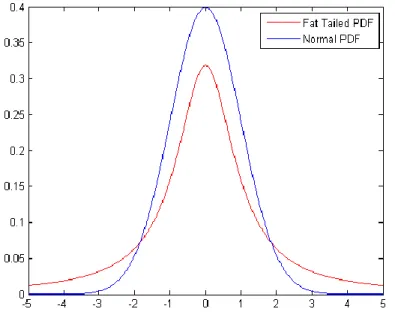
However, before starting EVT, it is important to mention some properties of the financial data. In particular, it is by now well-known that returns on financial assets typically exhibit higher than normal kurtosis as expressed by both higher peaks and fatter tails than can be found in normal distribution.

Figure 1: Asset returns distribution versus normal distribution

In figure 1, the red graph (Fat Tailed PDF) refers to the returns of a financial asset. The graphic tells us that the probabilities that normal distribution assigns to extreme events (tail events) are less than is required. In other words, the tails of the normal distribution are too thin to address the extreme losses or gains, assuming normality will lead to systematic

(20)

8

1 _{Theoretical background formulas are presented for only the maximum returns, since we can obtain the formulas for the minimum returns} with the opposite: Hn(r) = Min(r1,...,rn) = -Max (-r1,…,-rn)

underestimation of the riskiness of an asset and increase the chance of having a hit. Thus, in order to get rid of such kind of problems, tails of the distribution must be modeled. This can be done by using EVT.

Within the EVT context, there are three approaches to modeling the extremal events: the first one for directly modeling the distribution of maximum/minimums returns named Block Maxima, the second one for modeling the exceedances of a particular estimated threshold named Peak-Over-Threshold (POT), and the third one denominated Peaks-Over-Random-Threshold (PORT).

The Block Maxima, which is used for the largest observations that are collected from large samples of identically and distributed observations (i.i.d), is a method that provides a model that may be appropriate for the monthly or annual maximum/minimums of such samples. The second method is the Peaks-Over-Threshold, which is used for all large observations that exceed a high threshold. They are considered to be the most useful methods for practical applications because of their more efficient use of the data on extreme values. The third method is the most recent of all and it is denominated Peaks-Over-Random-Threshold, which is a small variant of POT, where the threshold is a random variable.

When modeling the maxima/minima of a random variable, extreme value theory follows the same fundamental role as the central limit theorem follows when modeling sums of random independent variables. In both cases, the theory tells us what the limiting distributions are.

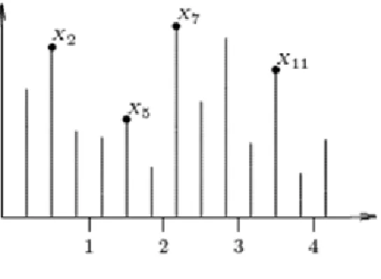
3.1 The Block Maxima Approach

Let‟s consider a random variable representing monthly maximum/minimum returns, which takes in successive periods. These selected observations constitute the extreme events, also called block (or per period) maxima/minima. In figure 2, the observations X2, X5, X7and X11

(21)

9

Figure 2: Block-maxima graph

The block maxima method is the traditional method used to analyze data with seasonality, as for instance, hydrological data. However, the threshold method uses data more efficiently, and for that reason, seems to have become the method of choice in recent applications.

According to the theorems of Fisher and Tippett (1928) and Gnedenko (1943), regardless of the specific distribution, the appropriately scaled maxima converge to one of three possible limit laws (parametric distributional forms). Under certain conditions, a standardized form of the three limit laws is called the generalized extreme value (GEV) distribution. Additionally, as is explained below by the theorems of Balkema and de Haan (1974) and Pickands (1975), the distribution function of the excesses above a high threshold converges to the generalized Pareto distribution (GPD).

Therefore, the block maxima model can be presented under a single family which is known as the generalized extreme value (GEV) distribution. The theory deals with the convergence of maxima, that is, the limit law for the maxima. To illustrate this, suppose that rt, t =1,...,n, is a sequence of independent and identically distributed (i.i.d) observations with distribution function H

  

x Pr rtx



, not necessarily known, and let the sample maximum be denoted by

Mn = max {r1,…,rn} where n  2, and  denote the real line. More generally, the generalized

extreme value distribution (GEV) represented by Hξ(x) describes the limiting distribution of

suitably normalized maxima. The random variable X may be replaced by (X – μ)/σ to obtain a standard GEV with a distribution function that is specified as shown below, where μ, σ and ξ are the location, scale and shape parameters, respectively.

(22)

10 The function H can belong to one of the three standard extreme value distributions:

 





















0

0 ,

exp

0 ,

0 :

Fréchet



x

 

          



0 0 , 1 0 , ( exp : Weibull

)

   x x x

x

 







  x



x,x :

Gumbel

exp

However, instead of having three functions, Jenkinson (1955) and Von Mises (1954) suggested the following distribution:

 





              0 (exp) 0 1

exp

1      if x if x x H

This generalization, known as the generalized extreme value (GEV) distribution, is obtained by setting ξ = 1

> 0 for the Fréchet distribution, ξ = 1< 0 for the Weibull distribution and by interpreting the Gumbel distribution as the limit case for ξ = 0. (Note that α refers to the tail index, which is the inverse of the shape parameter, which is defined as α = ξ-1).

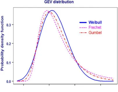
The shapes of the probability density functions for the standard Fréchet, Weibull and Gumbel distributions are given in figure 3.

(1)

(2)

(3)

(23)

11

Figure 3: Densities for the Fréchet, Weibull and Gumbel functions

We observe that the Fréchet distribution has a polynomial decaying tail and therefore suits heavy-tailed distributions well. The exponentially decaying tails of the Gumbel distribution characterize thin-tailed distributions. Finally, the Weibull distribution is the asymptotic distribution of finite endpoint distributions.

As in general it is not possible to know in advance the type of limiting distribution of the sample maxima, the generalized representation is particularly useful when maximum likelihood estimates have to be computed. Moreover, the standard GEV defined in (4) is the limiting distribution of normalized extremes, given that in practice the true distribution of the returns is not known, and as a result, we used the three parameter specifications

 





                 _ __                          0 , 0 , 0 , , , ,                x H x x D D H

of the GEV, which is the limiting distribution of the normalized maxima.

The class of distribution of H

 

x where the Fisher-Tippett theorem holds is quite large. One of the conditions is that H

 

x has to be in the domain of attraction of the Fréchet distribution (ξ > 0), which in general holds for the financial time series. Gnedenko (1943) shows that if the tail of H

 

x decays like a power function, then it is in the domain of attraction of the

(24)

12 Fréchet distribution. The class of distributions whose tails decay like a power function is large and includes Pareto, Cauchy, Student-t, which are the well-known heavy-tailed distributions.

3.2 Peaks-Over-Threshold Approach (POT)

The second approach focuses on the realizations exceeding a given (high) threshold. The observations X1, X2, X7, X8, X9and X11in the figure 4, all exceed the threshold u and constitute

extreme events.

Figure 4: Excesses over a threshold μ graph.

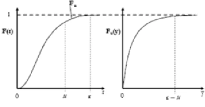
In general, we are not only interested in the maxima/minima of observations, but also in the behavior of large observations that exceed a high threshold. One method of extracting extremes from a sample of observations,rt, t = 1, 2,...,n with a distribution function

  

x r x



F Pr t is to take exceedances over a deterministic predetermined high-threshold u (figures 4 and 5). Exceedances of a threshold u occur whenrt > u for any t in t = 1,..., n. An excess over u is defined by y =ri– u.

(25)

13 Given a high threshold u, the probability distribution of excess values ofrtover threshold u is defined by

 

Pr



|



Fu y  r u y ru

This represents the probability that the value of r exceeds the threshold u by at most an amount y given that r exceeds the threshold u. This conditional probability may be written as

 

r



_

_







_{ }

 

r P , P 1 u r u y r u F y u F u F y r u F u         

Since x = y + u for r > u, we have the following representation:

 

1

 

u

 

F x  _ F u _F y F u Notice that this representation is valid only for ru.

A theorem due to Balkema and de Haan (1974) and Pickands (1975) shows that for sufficiently high threshold u, the distribution function of the excesses may be approximated by GPD, because as the threshold gets large, the excess Fu y

 

converges to the GPD.

The GPD in general is defined as

 

  1/ , , / 1 0 1 0

1 exp

u x u if G x if

x u

     





              





_











With (9)



,



, 0 , , 0 u if x u u if





_



      _  _   _ _  (8) (6) (7) (10)

(26)

14 Where σ and ξ are the scale and shape parameters, respectively. There is a simple relationship between the standard GPD Gξ (x) and Hξ(x) such that Gξ (x)= 1+log Hξ(x) if log Hξ(x) > -1.

The GPD embeds a number of other distributions; the ξ (shape parameter) determines the original distribution. When u = 0 and σ = 1, and ξ > 0, the tail of the distribution function F of

x decays like a power function x1/. In this case, F belongs to a family of heavy-tailed distributions that includes, among others, the Pareto, log-gamma, Cauchy and t-distributions; it takes the form of the ordinary Pareto distribution. This particular case is the most relevant for financial time-series analysis, since it is a heavy-tailed distribution.

For ξ = 0, the tail of F decreases exponentially, and belongs to a class of medium-tailed distributions that includes the normal, exponential, gamma and log-normal distributions. Finally, for ξ <0, the underlying distribution F is characterized by a finite right endpoint, whose class of short-tailed distributions includes the uniform and beta distributions.

The shapes of the probability density functions for the standard Beta, Pareto and Exponential distributions are given in figure 6.

Figure 6: Densities for the Beta, Pareto and Exponential functions

The importance of the Balkema and de Haan (1974) and Pickands (1975) results is the fact that the distribution of excesses may be approximated by the GPD by choosing ξ and setting a high threshold u. The GPD model can be estimated by using the parametric methods, explained below.

(27)

15

3.3 Peaks-Over-Random Threshold Approach (PORT)

Another method, and the most recent one, is denominated Peaks-Over-Random-Threshold (PORT). It is a semi-parametric method that is a small variant of POT, a method which is conditioned by a random threshold.

As we do not have an accurate choice of the threshold level, this new method introduces a new approach to dealing with this problem. Theory tells us that the threshold level should be high in order to satisfy the Pickands-Balkema-de Haan theorem, but the higher the threshold, the fewer observations are left for the estimation of the parameters of the tail distribution function.

In this method, any inference concerning the tail of the underlying distribution is based exclusively on the observations above a random threshold. This method compares with the alternative method of the number of observations that exceed a given high increasing deterministic level u, an approach named POT method.

Recently, Neves et al. (2006) and Neves and Fraga Alves (2007) have introduced two testing procedures that are based on the sample observations above a random threshold, procedures that consist in a reformulation of the asymptotic properties of the Hasofer and Wang (1992) test statistic.

3.4 Parameter Estimation Methods

In this section we explain the statistical parameter estimation of the distributions. Two approaches are considered. The first one, where the parameters of the distribution, including the tail index, are directly estimated by classical methods such as the maximum likelihood estimate method (MLE), is named the parametric approach. The second, where no parametric distribution is assumed for the extremes, is named the non-parametric approach.

3.4.1. The parametric approach

The parametric approach assumes that maximum/minimum returns selected over a given period are exactly drawn from the extreme value distribution given by GEV (see formula 4), or alternatively, that those positive/negative return exceedances under or above a given threshold are exactly drawn from the distribution given by the GPD formula (see formula 9).

(28)

16 With either definition of extremes, the asymptotic distribution contains three parameters: μ, σ and ξ for extremes defined as maximum/minimum returns selected from a period containing n returns.

Under the assumption that the limit distribution holds, the maximum likelihood method gives unbiased and asymptotically normal estimators. The system of non-linear equations can be solved numerically using the Newton–Raphson iterative method. Both distributions are parameterized by the scale, location and shape parameters with the same interpretation in both cases. This method maximizes the likelihood function over the location, scale and shape parameters: μ, σ and ξ.

In practice, with MLE the parameters of the extreme value distributions can be estimated with different values of the number of returns contained in the selection period n (for maximum/minimum returns) and alternatively, with different values of the threshold μ (for positive/negative return exceedances).

Mathematically, this solves the general formula presented below:

               















_

















_



          n i i n i i n

x

L 1 1

1

/ 1 exp 1 / 1 1 , ,















    

The estimates of μ, σ and ξ – sayˆ , ˆ and ˆ – are taken to be those values which maximize the likelihood L.

However, this methodology presents some limitations. Maximum likelihood methods perform better when tails are thicker, providing greater observations exceeding the threshold. Any weaknesses in these assumptions directly affect the significance of the results. Jansen and de Vries (1991) show that in the Fréchet domain of attraction this includes most distributions of financial returns. Maximum likelihood methods are consistent, but not the most efficient. Therefore, in some situations we should use parametric methods that are alternatives to the Maximum Likelihood Estimate Method (MLE), such as the method of Probability Weight Moments (PWM). However, in this thesis we focus only on the first one.

(29)

17

3.4.2. The non-parametric approach

The parametric approach method assumes that the parameters are drawn exactly from the extreme value distribution. However, the non-parametric approach assumes that estimator for the shape parameter ξ, which do not assume that the observations of extremes follow exactly the extreme value distribution, have been developed by Pickands (1975) and Hill (1975). Pickands’s estimator is given by

1 2 1 2 1 4 1 1 ' ' ln ln 2 ' ' n q n q Pickands n q n q R R R R



             _ _   

where (R‟t)t = 1, N is the series of returns ranked in an increasing order and q is an integer

depending on the total number of returns contained in the database n. Pickands‟s estimator is consistent if q increases at a suitably rapid pace with n. Pickands’s statistic is asymptotically normally distributed with mean ξ and variance ξ2.

Hill’s estimator is given by





1 1 1 1 ln ' ln ' 1 q Hill n n q i R R q        _ _    



Where R'N1 denotes decreasing order statistics of the series and q denotes the q th

smallest order statistic of n observations included in the calculation of the shape parameter. Intuitively the Hill index measures the distance with which the average extreme observation exceeds a specific threshold.

However, the Hill estimator has some weaknesses. Dekkers and De Haan (1990), who take into account the sensitivity of the Hill index to the initial tail size, propose an extension to the Hill estimator incorporating its second moment.





                   2 1 2 1 1 ker 1 2 1 1 Hill Hill Hill s Dek    

Where ξ Hill 1 is the standard Hill estimate defined in equation (12) and





2 1 2 n 1 n q 1 1 1

lnR'

R'

q Hill i q          _   





(12) (14) (15) (13)

(30)

18 The authors prove the consistency and normality of ξ Dekkers.

In summary, the problem consists of choosing the correct method to obtain the correct value for the tail index parameter. As largely discussed in the extreme value theory literature, the choice of its value is a critical issue. The origin of this problem comes from the fact that the database contains a finite number of maximum/minimum return observations; the number of extreme returns, q, used for the estimation of the model is finite.

On one hand, choosing a high value for q leads to few observations of extreme returns and implies inefficient parameter estimates with large standard errors. On the other hand, choosing a low value for q leads to many observations of extreme returns but induces biased parameter estimates as observations not belonging to the tails are included in the estimation process.

This sensitive tradeoff can be dealt with in a variety of ways, as was described above. However, in recent years new approaches have been developed. One of them is when the levels at which the tail index begins to plateau is in some sense the „optimal‟ choice of n where it is no longer as sensitive to individual observations. Other approaches to making this choice include the quantile–quantile plot, regression methods (Huisman et al., 2000) and the subsample bootstrap (Danielsson and de Vries 2001).

(31)

19

4. Empirical Application

In this section we proceed to the application of the GEV and GPD distributions to our database, which is composed of the monthly maximum and minimum returns of the FTSE100, NIKKEI225 and S&P500 indices. The goal is to fit our maximum and minimum return series to the GEV and GPD distributions.

There will be a description of the methodology that we adopted, an empirical analysis of our database, and finally, the application of the GEV and GPD distributions.

4.1 Methodology

In this thesis, we applied some of the theory presented above, such as the Block Maxima and POT approaches. We also applied parameter estimation methods such as the MLE method, which uses a parametric approach, and the Hill estimator, which uses a non-parametric approach. The goal is to fit our maximum and minimum return series to the GEV and GPD distributions.

For the application of the methodology, we used a diversity of tools such as the language R with an extRemes toolkit, whose outputs and code can be seen in the appendix. Another tool that we used was the Easy Fit 5.5 Professional Software, which is a powerful tool in terms of graphs. Finally, we used the EViews Software.

The data consist of the monthly maximum and minimum log returns from the FTSE100, NIKKEI225 and S&P500 indices. The monthly maximum and minimum refers to the maximum and minimum return, extracted from the daily log return, in each month for each index.

In terms of log return series, assuming that Pt is the closing value on day t, continuous daily logarithmic returns are given by:

 t R 1 ln t t P P       

The data that we considered were downloaded from the Yahoo Finance webpage. The period under analysis for the S&P 500 index is from January 3, 1950 to March 11, 2011. The FTSE

(32)

20 100 index corresponds to a period between February 4, 1984 and March 11, 2011, and the NIKKEI 225 index corresponds to the period between January 4, 1984 and March 11, 2011.

4.2 Empirical Results

In this section, we proceed to an exploratory data analysis, followed by the application of the Block Maxima and POT approaches.

To start, tables 1, 2 and 3 show the summary statistics of the daily log returns and monthly maximum (Max) and minimum (Min) log return series of the FTSE100, NIKKEI 225 and S&P500 indices.

Data FTSE 100 - Daily FTSE 100 - Min FTSE 100 - Max

Observations 6807 324 324 Mean 0.0002 -0.0191 0.0189 Median 0.0006 -0.0161 0.0150 Maximum 0.0938 -0.0045 0.0938 Minimum -0.1303 -0.1303 0.0057 Std. Dev. 0.0112 0.0126 0.0117 Skewness -0.3850 -3.4470 2.8954 Kurtosis 11.7930 24.6915 14.8249 Jarque-Bera 22097.09 6993.67 2340.40 Probability 0.0000 0.0000 0.0000

Table 1: FTSE 100 Explanatory data analysis

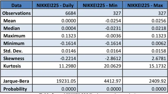
Data NIKKEI225 - Daily NIKKEI225 - Min NIKKEI225 - Max

(33)

21

Data S&P500 - Daily S&P500 – Min S&P500 – Max

Table 3: S&P 500 Explanatory data analysis

Looking at table 1, it is possible to see that in the daily return the stock index FTSE100 has a mean of 0.02% and a standard deviation of 1.12%, with a maximum of 9.38% and a minimum of -13.03%. In terms of the maximum returns, the series has a mean of 1.89% and a standard deviation of 1.17%, with a maximum return of 9.38% and a minimum of 0.57%. In the minimum return FTSE 100, the series has a mean of -1.91% with a standard deviation of 1.26%, and a maximum of -0.45% and a minimum of -13.03%.

In the other stock index, the NIKKEI 225, we can see that in the daily return the series has a mean of 0.00% and a standard deviation of 1.46%, with a maximum of 13.23% and a minimum of -16.14%. In terms of the maximum returns, we can see that the series has a mean of 2.56% and a standard deviation of 1.58%, with a maximum return of 13.23% and a minimum of 0.62%. In the minimum return of the NIKKEI 225, the series has a mean of 2.54% with a standard deviation of 1.64%, a maximum of 0.36% and a minimum of -16.14%.

In the last stock index, the S&P 500, in terms of daily return the index has a mean of 0.03% and a standard deviation of 0.97%, with a maximum of 10.96% and a minimum of -22.90%. In terms of the maximum returns, it has a mean of 1.67% and a standard deviation of 1.00%, with a maximum return of 10.96% and a minimum of 0.29%. Finally, the minimum S&P 500 return has a mean of -1.65% with a standard deviation of 1.36%, a maximum of -0.18% and a minimum of -22.90%.

(34)

22 On the other hand, these tables show that the kurtosis and skewness values are very different from 3 and 0, respectively, for the distribution to be considered a normal distribution. However, in addition to this method, another way to prove the normality of a distribution is the Jarque-Bera (JB) test, which depends on the skewness and kurtosis estimates. Based on the JB test, it is possible to conclude if the normality assumption is rejected or not, depending on the probability associated with the test. If it is lower than 0.05 (the default significance level assumed for all tests in this thesis), we reject the null and the normality assumption; otherwise, we can admit the normality based on the considered sample.

       on Distributi Normal H on Distributi Normal H Test JB 1 0

For the FTSE 100, NIKKEI 225 and S&P 500 series we can see that daily log returns and the monthly maximum and minimum log return series distributions do not follow a normal distribution, because in all cases we reject the null hypothesis in the JB test, as a consequence of the associated probability of the JB test being lower than 0.05.

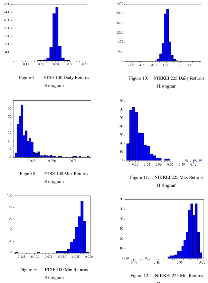
In the figures below, it is possible to see that none of the histograms of the daily log returns and the monthly maximum and minimum log returns of the FTSE 100 (figures 7 – 9), NIKKEI 225 (figures 10-12) and S&P 500 (figures 13 – 15) seem to follow the normal distribution, which is confirmed by the rejection of the null hypothesis in the JB test.

In the figures below it is also possible to see and analyze the graph of the adjust close of the FTSE 100 (figure 16), NIKKEI 225 (figure 20) and S&P 500 (figure 24), as well as the daily log return and the monthly maximum and minimum returns graphs.

(35)

23

Figure 7: FTSE 100 Daily Returns Histogram

Figure 8: FTSE 100 Max Returns Histogram

Figure 9: FTSE 100 Min Returns Histogram

Figure 10: NIKKEI 225 Daily Returns Histogram

Figure 11: NIKKEI 225 Max Returns Histogram

Figure 12: NIKKEI 225 Min Returns Histogram

(36)

24

Figure 13: S&P 500 Daily Returns Histogram

Figure 14: S&P 500 Max Returns Histogram

Figure 15: S&P 500 Min Returns Histogram

Figure 16: FTSE 100 Adjust Close

Figure 17: FTSE 100 Daily Return

Figure 18: FTSE 100 Monthly Maximum Return

(37)

25

Figure 19: FTSE 100 Monthly Minimum Return

Figure 20: NIKKEI 225 Adjust Close

Figure 21: NIKKEI 225 Daily Return

Figure 22: NIKKEI 225 Monthly Maximum Return

Figure 23: NIKKEI 225 Monthly Minimum Return

(38)

26

Figure 25: S&P 500 Daily Return

Figure 26: S&P 500 Monthly Maximum Return

Figure 27: S&P 500 Monthly Minimum Return

(39)

27

4.3 Fitting the GEV Distribution

In this section we will determine which one of the extreme value distributions is more appropriate for modeling the monthly maximum/minimum returns of the FTSE 100, NIKKEI 225 and S&P500 indices under analysis, applying the GEV distribution using the MLE parametric approach.

We start with the LR test (Likelihood Ratio test) and the Log-Likelihood value for each of the series.

Based on the LR test, it is possible to conclude if the Gumbel distribution assumption is rejected or not, depending on the probability associated with the test. If it is lower than 0.05, we reject the null and the Gumbel distribution assumption; otherwise, we can admit the Gumbel distribution based on the considered sample.

       on Distributi Gumbel H on Distributi Gumbel H Test LR 1 0

Likelihood Ratio Test p-value Negative Log-likelihood

FTSE100 -Max Return 65.42 6.051E-16 -1125.03

FTSE100 -Min Return 603.54 2.850E-133 -1064.76

NIKKEI 225 -Max Return 30.51 3.318E-08 -993.17

NIKKEI 225 -Min Return 512.95 1.443E-113 -956.08

S&P 500 -Max Return 56.84 4.734E-14 -2564.37

S&P 500 -Min Return 1995.90 0.000E+00 -2426.38

Table 4: LR Test and Log-Likelihood Results - GEV

For a LR test, we reject the null hypothesis. This means that we do not assume that the series follows a Gumbel process. Therefore, we can conclude that none of the maximum/minimum return series have been generated by a Gumbel distribution. This means that for the considered series, only the Fréchet or Weibull particular cases of the more general GEV distribution remain.

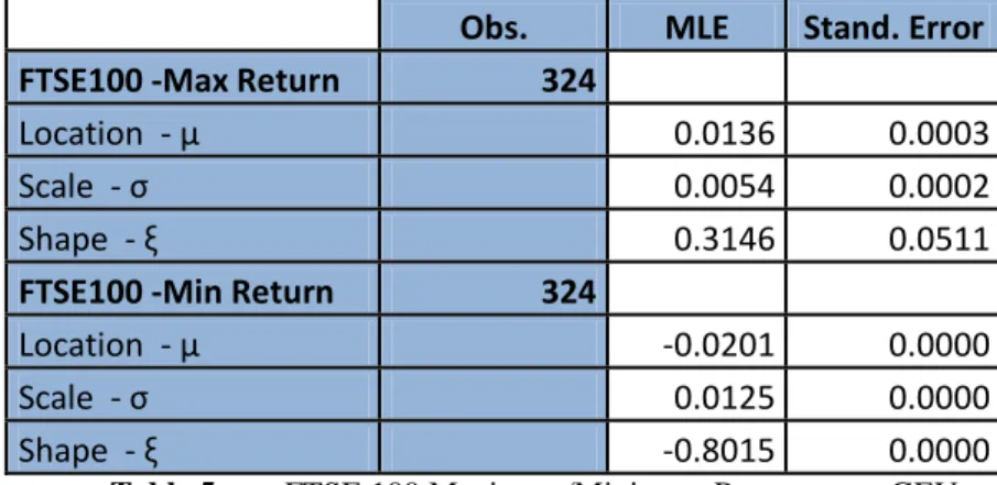
Studying each series individually now, and starting with the monthly maximum and minimum series of the FTSE 100 index, using the MLE, we found the optimal values for the parameter estimates, which we present next:

(40)

28

Obs. MLE Stand. Error

FTSE100 -Max Return 324

Location - μ 0.0136 0.0003

Scale - σ 0.0054 0.0002

Shape - ξ 0.3146 0.0511

FTSE100 -Min Return 324

Location - μ -0.0201 0.0000

Scale - σ 0.0125 0.0000

Shape - ξ -0.8015 0.0000

Table 5: FTSE 100 Maximum/Minimum Parameters - GEV

For the FTSE 100 maximum returns, we conclude that the Fréchet distribution (a common result in empirical finance) seems to be the most appropriate to describe that kind of data, as the shape (ξ) estimate is higher than zero. Consequently, we can conclude that FTSE 100 maximum return empirical distribution has fat tails. The larger the estimate values for the shape parameter, the more fat-tailed the distribution. We can see the representation of the distribution in figure 30.

For the maximum return series, the Probability Plot (PP) (figure 28) and the Quantile Plot (QQ) (figure 29) seem to confirm that the data has been generated by the Fréchet distribution, as the points are near the straight line. In both graphs we are comparing the returns series (data) against the Fréchet distribution.

For the FTSE 100 minimum returns, it is possible to see that we have a Weibull distribution, because the shape estimate (ξ) is lower than zero. We can see the histogram with the Weibull density function in figure 34.

For the minimum return series, we can see in the Probability Plot (PP) (figure 32) that the series could be generated by a Weibull process, since the graph is approximately linear. On the other hand, the Quantile - Quantile Plot (QQ) (figure 33) confirms the PP plot, since the observed data (series) tend to concentrate around the straight line, which confirm the Weibull goodness-of-fit. In both graphs we are comparing the series (data) empirical distribution against the theoretical Weibull distribution.

Therefore, in terms of monthly maximum and minimum FTSE 100 series, we can admit the series have been generated by Fréchet and Weibull process distributions, respectively.

(41)

29

Figure 28: FTSE100 Max Return Fréchet Probability Plot

Figure 29: FTSE100 Max Return Fréchet Quantile Plot

Figure 30: FTSE100 Max Return Density Plot

Figure 31: FTSE100 Max Return Density Plot II

Figure 32: FTSE100 Min Return Weibull Probability Plot

Figure 33: FTSE100 Min Return Weibull Quantile Plot

Figure 34: FTSE100 Min Return Density Plot

Figure 35: FTSE100 Min Return Density Plot II

(42)

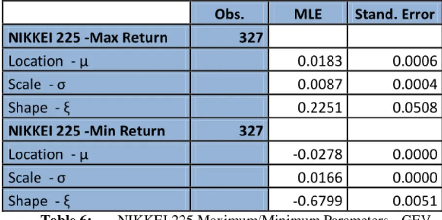
30 Now analyzing the monthly maximum and minimum return series of the NIKKEI 225 index, we found the optimal values for the parameter estimates, which we present next:

Obs. MLE Stand. Error

NIKKEI 225 -Max Return 327

Location - μ 0.0183 0.0006

Scale - σ 0.0087 0.0004

Shape - ξ 0.2251 0.0508

NIKKEI 225 -Min Return 327

Location - μ -0.0278 0.0000

Scale - σ 0.0166 0.0000

Shape - ξ -0.6799 0.0051

Table 6: NIKKEI 225 Maximum/Minimum Parameters - GEV

For the NIKKEI 225 maximum returns, we conclude that the Fréchet distribution seems to be the most appropriate to describe that kind of data, as the shape (ξ) estimate is higher than zero. Therefore, we can conclude that NIKKEI 225 maximum return empirical distribution has fat tails. We can see the representation of the distribution in figure 38.

For the maximum return series, the Probability Plot (PP) (figure 36) and the Quantile Plot (QQ) (figure 37) seem to confirm that the data has been generated by the Fréchet distribution, as the points are near the straight line. In both graphs we are comparing the returns series (data) against the Fréchet distribution.

For the NIKKEI 225 minimum returns, it is possible to see that we have a Weibull distribution, because the shape estimate (ξ) is lower than zero ( ˆ = -0.67366). We can see the histogram with the Weibull density function in figure 42.

For the minimum return series, we can see in the Probability Plot (PP) (figure 40) that the series could be generated by a Weibull process, since the graph is approximately linear. On the other hand, the Quantile - Quantile Plot (QQ) (figure 41) confirms the PP plot, since the observed data (series) tend to concentrate around the straight line, which confirm the Weibull goodness-of-fit. In both graphs we are comparing the series (data) empirical distribution against the theoretical Weibull distribution.

Consequently, in terms of monthly maximum and minimum NIKKEI 225 series, we can admit the series have been generated by Fréchet and Weibull process distributions, respectively, as happened with the monthly maximum and minimum FTSE 100.

(43)

31

Figure 36: NIKKEI 225 Max Return Fréchet Probability Plot

Figure 37: NIKKEI 225 Max Return Fréchet Quantile Plot

Figure 38: NIKKEI 225 Max Return Density Plot

Figure 39: NIKKEI 225 Max Return Density Plot II

Figure 40: NIKKEI 225 Min Return Weibull Probability Plot

Figure 41: NIKKEI 225 Min Return Weibull Quantile Plot

Figure 42: NIKKEI 225 Min Return Density Plot

Figure 43: NIKKEI 225 Min Return Density Plot

How to deal with extreme observations in empirical finance: an application to capital markets