NEW RESULTS ON FRACTIONAL LINEAR PREDICTION

Abstract

A generalisation of the linear prediction for fractional

steps is reviewed, widening well-known concepts and

results. This prediction is used to derive a causal

interpolation algorithm. A reconstruction algorithm for

the situation where averages are observed is also

presented.

1 INTRODUCTION

The relevance of linear prediction in modern Signal Processing is a well-established fact. The one-step prediction has several practical applications, namely in Telecommunications and Speech Processing, for example, sampling rate conversion, equalization, and speech coding and recognition. The d-step prediction (d positive integer) is useful in Geophysical Signal Processing.

The basic idea underlying the proposed algorithm is to develop a system capable of linear predicting the signal over instant times, in between the current ones, without converting the signal to the continuous-time domain. The new samples would fit in between the original samples. The algorithm uses the Maximum Entropy Method to obtain the spectrum of the original integer sampled signal.

Using this spectrum estimate, it is possible to derive the coefficients of the fractional predictor. The simulations present in this work will show that, from the fractional linear prediction method, it is possible to perform the multirate conversion either for a higher or lower rate.

In section 2, a fractional delay and lead concepts review takes place. These concepts are the base for the theory of fractional linear prediction that is described in section 3. An algorithm is proposed, for the computation of the optimum predictor coefficients. In section 4, some examples to illustrate the behaviour of the algorithm, are presented. At last some conclusions are outlined.

2 FRACTIONAL DELAY AND LEAD

We will base our algorithm on the theory of the fractional linear systems [1].

The starting point is the definition of fractional delay and lead [1]:

xn+α=

[

]

[

]

∑

−∞

=

+

−

−

+

m m

m

n

m

n

x

α

π

α

π

(

)

sin

(2.1)

where α∈R and n∈Z. This equation expresses a relation between two signals xn and ym = xn+α

defined in the sets Z and { m: m=n+α, n∈Z and

α∈R}, respectively. So, we are relating two signals defined over two different time grids, obtained, one from the other by a fractional translation. The

NEW RESULTS ON FRACTIONAL LINEAR PREDICTION

Manuel D. Ortigueira Carlos J. C. Matos

Instituto Superior Técnico/INESC and UNINOVA

Campus da FCT da UNL, Quinta da Torre, 2825 - 114 Monte da Caparica, Portugal,

Mail: [email protected]

UNINOVA and Escola Superior de Tecnologia, Instituto Politécnico de Setúbal,

relation (2.1) is a convolution of x

nand a δn+a given

by:

δn+a=

sin[π(α+n)] [π(α+n )] =

sin(πα)

πα

(-1)n

1+_αn

(2.2)

which can be considered as the impulse response of a reconstruction filter, δn+a, such that

xn+α = xn*δn+a (2.3)

Applying the Fourier Transform (FT) to both members of equation (2.1) and putting Xα(ejω) = FT[xn+α], we obtain:

Xα(ejω) = ejωα X(ejω) (2.4) thus generalising a well-known result.

The previous relations are the bases for the d-step prediction we will present in the following section. The d-step prediction can be used to interpolate a signal, allowing us to convert a signal defined in a given uniform time grid into another one. We will show how to compute the predictor parameters according to the spectral properties of the signal. The situation of lack of knowledge of these properties is also addressed.

3 D-STEP PREDICTION

In [1,2], a generalisation of the notion of linear prediction for any fractional d-step prediction (d≤1), but without any details, was proposed. We will now go into the details of this topic. We shall be working in the context of a stationary real stochastic process. Let x(n) n∈Ζ be such processes and let Rx(k) be its

autocorrelation function.

Definition 3.1

Let x(n) be a real stationary stochastic process, observed from -∞ to n-1. We define the Nth order d-step prediction at n-1+d (0<d≤1) by:

x^(n-1+d) = -

∑

i=1 N

ai x(n-i) (3.1)

where ai (i=1, ..., N) are the coefficients of the

d-step predictor (d=1, corresponds to the usual

one-step prediction). The predictor coefficients will be chosen in order to minimise the prediction error power:

Pd = E[

(

)

Theorem 3.1 - According to the previous definition and assuming that the correlation matrix of x(n)

has, at least rank N, the optimum d-step predictor is

given by the solution of the following set of normal

equations[1,2]:

∑

ai.Rx(k-i) = -Rx(-k-d-1) k=1,2,…, N (3.3)

or, in a matrix format:

Rx.a=-rd (3.4)

where the meaning of the vectors and matrix is evident. The corresponding minimum error power is easily obtained by inserting (3.3) in (3.2) and it is given by:

Pdmin = R(0) +

∑

i=1 N

ai.R(-i-d+1) (3.5)

Now, let pn

i (i=0,1, ..., n), with p n

0 = 1 , be the n

th

order one-step linear predictor coefficients and Pn(z) the corresponding Z Transform. As it is well known, the predictors allow us to obtain the Cholesky factorisation for the inverse of the Toeplitz matrix, RN, in (8) [4]:

R-1

N = P.D.P

H

(1) (3.6)

where P is a lower triangular matrix having the one-step predictors as columns, D is a diagonal matrix with the inverses of the one-step prediction error powers.

The substitution of (3.6) into (3.4) allows us to express the a’s in terms of the one-step predictor coefficients. It is not hard to show that:

a = P.v (3.7)

with v given by:

v = D.PH.rd (3.8)

where rd is the vector in the right hand side in

R(-k-d+1)=

R(k-1+d)=sin(πd)

πd .

∑

-∞

∞

R(n) (-1)

k-1-n

α+k-1-n (3.9)

But, as the autocorrelation function is an even function, we can transform the previous equation into:

R(-k-d+1) = R(k-1+d) =

(-1)k-1sin(πd)

π( α+k-1) .

















R(0)+ 2

∑

(-1)

n _R(n)

1-

_



_



2 (3.10)

Since the coefficients go to zero, at least quadratically, the series converges quickly, allowing its truncation.

So, with equations (3.4) and (3.10) we can compute the coefficients of the fractional predictor, provided that we use a suitable autocorrelation function estimate.

The use of the Z Transform in (3.7) lead to an interesting result:

A(z)=

∑

i=1 N

vi.z-i PN-i(z) (3.11)

where Pk(z) is the kth order prediction error filter transfer function and the vi are the components of

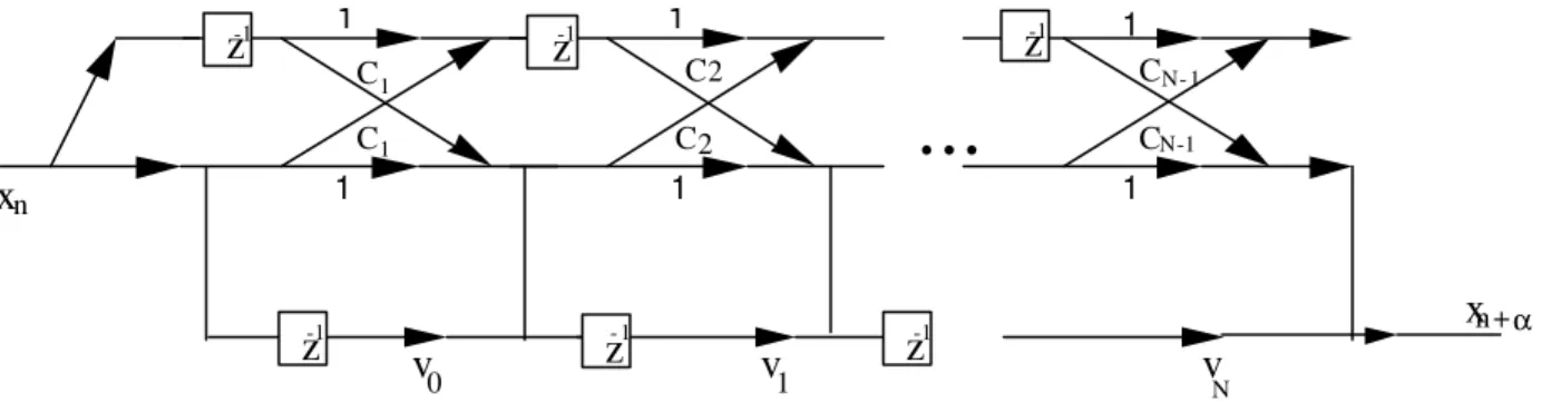
the vector v defined in (3.8). The result (3.11) is important, since it shows that the predicted value is a linear combination of all the forward prediction error signals {fig.1} (2).

1

H means conjugate transpose.

2

Instead of the Cholesky factorisation we could use the Gohberg-Semencul formula [6]. In this case,

Assume now that x(n) is an AR(N-1) stationary stochastic process. Then the longest (with greater order) optimum fractional d-step predictor has order N [2].

This allows us to devise a better way to compute R(k+d). As the process is AR(N-1), the (N-1)th one-step predictor defines, together with the prediction error, PN-1, the spectrum of the process

[3,4]:

Sx(ω) = ₂

1

0 1

1

∑

=

− −

−

⋅

N

n

jwn N

i N

e

P

P

(3.12)

that can be used to obtain R(k+d):

R(k+d) = FT-1

[

]

With these results we can take advantage of the well-known linear prediction methods (e. g. modified covariance or Burg algorithms) [3,4]. The proposed algorithm has the following steps:

1 - Compute the N-1 linear predictors using a suitable algorithm.

2 - Use the (N-1)th linear predictor to estimate the spectrum, Sx(ω), and the

A(z) would be expressed in terms of the (N-1)th order forward and backward predictors, only, but the “coefficients” of the linear combination would be polynomials in z. A direct application of the Levinson algorithm would allow obtaining A(z) recursively (this will be done in a future work). The approach used here has some advantages that will be clear in the following.

z

C C

1 1

C C

C C

...

N- 1

z

z

2 2

N-1

z

_v

z

z

1

0

v

v

x

n +α

x

1

1

1 ₁

1 1

corresponding autocorrelation, of the signal.

3 - Multiply Sx(ω) by ejdω and compute the

inverse Fourier Transform to obtain the vector rd.

4 - Use (3.4) to obtain the coefficients of the fractional predictor.

This algorithm is simple and computationally efficient. Although obtained under the hypothesis that the signal is AR(N-1), it will be useful in other situations, namely in the ARMA case.

To illustrate the application of the method, we present some simulation results. We proceed in the following way:

a) Generate a signal with L points and a given signal to noise ratio;

b) Downsample it by 1/2 factor;

c) Use the previous algorithm to estimate the removed values;

d) Compute the error between each original and estimated value and the corresponding error power.

In the following pictures we present the results of two simulations using sinusoidal and non-sinusoidal data.

15 20 25 30 35 40 45 -3

-2 -1 0 1 2

O r i g i n a l a n d p r e d i c t e d v a l u e s p r e d i c t o r o r d e r = 6 S / N = 3 9 . 7 8 7 5 d B

Amplitude

S a m p l e s

P r e d i c t e d V a l u e s O r i g i n a l V a l u e s P r e d i c t o r u s e d v a l u e s

20 25 30 35 40 45 -0.05

0 0 . 0 5 0.1 0 . 1 5

S a m p l e s

Amplitude

D i f f e r e n c e s A v e r a g e P o w e r = 0 . 0 0 0 6 9 4 0 4 D i f f e r e n c e s b e t w e e n o r i g i n a l a n d p r e d i c t e d v a l u e s

Figure 2 – Fractional prediction of sinusoidal data

25 30 35 40 45 50 55 60

-2 -1 0 1 2

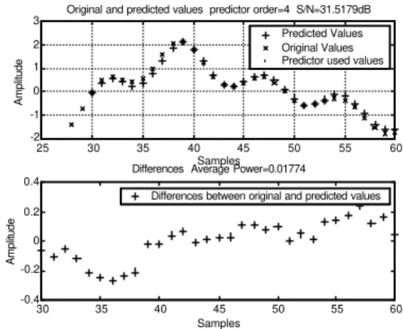
3 Original and predicted values predictor order=4 S/N=31.5179dB

Amplitude

Samples

Predicted Values Original Values Predictor used values

30 35 40 45 50 55 60

-0.4 -0.2 0 0.2 0.4

Samples

Amplitude

Differences Average Power=0.01774

Differences between original and predicted values

Figure 3 – Fractional prediction of a sum of sync

functions

For several predictor lengths we computed the corresponding prediction error power obtaining the results in table 1.

4 6 8 12 24

0.0177 0.0126 0.0093 0.0010 0.0047

Table 1 – error power as function of the predictor length

Obviously, we are not restricted to d=0.5. Consider that d assumes 3 values, d=0.25, d=0.5, d=0.75, and keep the predictor of order 4. We insert 3 values between each set of two original values. The results obtained are displayed in figure 4. As it is easy to conclude, we were making a rate increase by integer values. Of course, we can obtain a fractional rate increase (or decrease) by decimation.

5 10 15 20 25 30 35 40

-2 -1.5 -1 -0.5 0 0.5 1 1.5 2

Predicted Values Original Values

Figure 4 – interpolation using fractional prediction with

4 RECONSTRUCTION FROM

MA

MEASUREMENTS

We are going to propose a solution for an interesting problem. Let us assume that instead of observing the stochastic process x(n) for n∈Z, we observe an MA obtained as:

y(n) =

∑

i=0 M

bi x(n-iα) (4.1)

The problem we want to solve is:

Can we “recover” the unobserved values x(n-iα) for i=0, …,M?

The answer is positive. Let us see how we obtain the referred values. The procedure is similar to the one followed in section 3.

Definition 4.1

Let y(n) be a real stationary stochastic process,

observed from -∞ to n-1 and satisfying (4.1). We

define the Nth order d-step prediction of x(n) from

y(n) at n+lα (0<α<1 and l=0, …,M) by:

x^(n+lα) = -

∑

i=1 N

ai y(n-i) (4.2)

where ai (i=1, ..., N) are the coefficients of the lα

-step predictor.

As seen, this is a generalisation of the problem solved in section 3. If we put M=0, y(n)=x(n) and we return back to the normal d-step prediction. Of course, both filters in (4.1) and (4.2) can be noncausal. Again, the predictor coefficients will be chosen in order to minimise the prediction error power:

Pd = E[

(

)

Theorem 4.1 - According to the previous definition

the optimum lα - step predictor is given by the

solution of the following set of normal

equations[1,2]:

∑

i=1 N

ai.Ry(k -i) = -Rxy(-k-lα) k=1,2,…,N (4.4)

The minimisation of the prediction error power (4.3) is easily performed by differentiation of its right hand side in order to all the ai (i=1, ..., N) and

leads to the normal equations (4.4). As y(n) is obtained through an MA operation, the correlation matrix of y(n) has surely great than N rank. To compute the cross-correlation in (4.4), we define Sy(ejω) as the spectrum of y(n), Sxy(ejω) as the cross

spectrum and B(ejω) the frequency response of the MA filter in (4.1):

B(ejωα) =

∑

i=0 M

bk e-jkωα (4. 5)

We have too:

Sy(ejω) = B(ejωα). Sxy(ejω) (4. 6)

Thus

Rxy(-k-lα) = FT

-1

_[

_]

e-jωlαSyx(ejω) (4.7)

where Syx(ejω) = S

* yx(e

jω_{) . We must be careful when}

implementing (4.6), since the factors on the right have different periods. If we use a FFT with length L in the computation of Sy, we must use L/α when

computing B(ejωα), though only the first L points are used.

In the following figures, we illustrate the application of this algorithm. The signal used for the prediction was obtained from the original signal by substituting each pair of consecutive points by their average.

20 25 30 35 40 45 50

-2 -1 0 1 2

Original and predicted values predictor order=8 S/N=Inf dB

Amplitude

Samples

Predicted Values Original Values Predictor used values

20 25 30 35 40 45 50

-0.02 -0.01 0 0.01 0.02

Samples

Amplitude

Differences Average Power=7.1066e-005

Differences between original and predicted values

Figure 5 – Fractional reconstruction of sinusoidal

20 25 30 35 40 45 50 -2

-1 0 1 2

3 Original and predicted values predictor order=8 S/N=Inf dB

Amplitude

Samples

Predicted Values Original Values Predictor used values

20 25 30 35 40 45 50

-0.2 -0.1 0 0.1 0.2

Samples

Amplitude

Differences Average Power=0.0039284

Differences between original and predicted values

Figure 6 – Fractional reconstruction of sync data

5 CONCLUSIONS

In this paper we proposed a generalisation of the usual linear prediction to fractional step linear prediction. This allows us to predict the value of a signal defined at a uniform time grid to any point between any two grid points. We presented some illustrating examples showing the use of the algorithm to perform a signal interpolation. In a future publication we will present quantitative results illustrating the performance of the algorithm. From the examples, we can confirm the algorithm ability to perform a rate conversion. Besides its performance the algorithm can be implement in a recursive way. On the other hand, giving a lattice form to the predictor turns out to be a simple task.

References

[1] Ortigueira, M. D. “Introduction to Fractional Signal Processing II: Discrete-Time Systems”, IEE Proc. On Vision, Image and Signal processing, No.1, February 2000

[2] Ortigueira, M. D., “An Introduction to The Fractional Linear Prediction” V Ibero-American Symposium on Pattern Recognition, Lisbon, Sep., 11-13, 2000, pp. 741-748

[3] Ortigueira, M.D. and Tribolet, J. M.,"Global versus local minimization in least-squares AR Spectral Estimation", Signal Processing, Vol.7, Nº 3, Dec. 1984. [4] Proakis, J. G. and Manolakis, D. G.