Orientador: Professor Doutor Mário Fernando José Eusébio, FCT-UNL Co-orientadores: Professora Doutora Isabel Alexandra Canento Esteves Esperança, FCT-UNL Professor Doutor José Paulo Mota, FCT-UNL

Mafalda Sofia Moura Moraes Izidro

Licenciatura em Engenharia Química e Bioquímica

Real-time Labview assessment on

adsorption systems

Dissertação para obtenção do Grau de Mestre em Engenharia

Química e Bioquímica

Orientador: Professor Doutor Mário Fernando José

Eusébio, FCT-UNL

Co-orientadores:

Professora Doutora Isabel Alexandra

Canento Esteves Esperança, FCT-UNL

Professor Doutor José Paulo Mota, FCT-UNL

Presidente: Professora Doutora Maria Madalena Alves Campos de Sousa Dionísio Andrade

Arguente: Doutor Rui Pedro Pinto Lopes Ribeiro Vogais: Professor Doutor Mário Fernando José Eusébio Professora Doutora Isabel Alexandra Canento Esteves Esperança

Mafalda Sofia Moura Moraes Izidro

Licenciatura em Engenharia Química e Bioquímica

Real-time Labview assessment on

adsorption systems

Dissertação para obtenção do Grau de Mestre em Engenharia

Química e Bioquímica

Orientador: Professor Doutor Mário Fernando José

Eusébio, FCT-UNL

Co-orientadores:

Professora Doutora Isabel Alexandra

Canento Esteves Esperança, FCT-UNL

Professor Doutor José Paulo Mota, FCT-UNL

Presidente: Professora Doutora Maria Madalena Alves Campos de Sousa Dionísio Andrade

Arguente: Doutor Rui Pedro Pinto Lopes Ribeiro Vogais: Professor Doutor Mário Fernando José Eusébio Professora Doutora Isabel Alexandra Canento Esteves Esperança

Real-time Labview assessment on adsorption systems.

Copyright © Mafalda Sofia Moura Moraes Izidro, Faculdade de Ciências e Tecnologia, Universidade Nova de Lisboa.

A Faculdade de Ciências e Tecnologia e a Universidade Nova de Lisboa têm o direito, perpétuo e sem limites geográficos, de arquivar e publicar esta dissertação através de exemplares impressos reproduzidos em papel ou de forma digital, ou por qualquer outro meio conhecido ou que venha a ser inventado, e de a divulgar através de repositórios científicos e de admitir a sua cópia e distribuição com objectivos educacionais ou de investigação, não comerciais, desde que seja dado crédito ao autor e editor.

i  

Dedicatória

Dedico este trabalho aos meus pais que sem eles nada disto seria possível.

i  

Agradecimentos

A realização deste trabalho só foi possível devido a inúmeras pessoas que estiveram presentes ao longo da elaboração deste trabalho directa e indirectamente.

De entre todas, destaco as seguintes:

Em primeiro lugar, aos meus orientadores, Prof. Dr. Mário Eusébio, Prof. Dra. Isabel Esteves e Prof. Dr. José Paulo Mota, pela orientação, disponibilidade, partilha de conhecimentos e ensinamentos técnicos transmitidos ao longo da realização deste estudo.

Não esquecendo, a D. Maria José Carapinha e a D. Maria da Palma Afonso, pelo carinho, simpatia, grande paciência e atenção sempre dispensadas.

À minha família e amigos pelo apoio, amizade e motivação transmitida durante a realização deste trabalho.

A todos Muito Obrigada!

i  

ABSTRACT

This work aims to develop a LabVIEW interface for monitoring, controlling and automate the simultaneous experimental determination of one adsorption isotherm of gas in two distinct solid adsorbents.

The magnetic suspension balance has two samples and this way it’s possible to determinate, simultaneously, the equilibrium adsorption for two different adsorbents. The developed software allows the registration of weight values and the control of the state of the balance, which has three main positions (ZP, MP1 and MP2). To determine a isotherm point is necessary for the system to reach the equilibrium. The software records the different values of ZP, MP1 and MP2, calculating the adsorbed mass values for each of the adsorbents. When the average of the adsorbed masses remain constant, the pressure value is changed and is possible to proceed with the determination of a new point isotherm.

The software was developed in LabVIEW utilizing a software previously developed for a balance with only one sample. The old software was built using just one interface, which made the process of changing routines and new programming interfaces complicated. It was developed a sketch of a new software, now built in five separate blocks .

To validate the interface for monitoring the magnetic balance, multiple tests were conducted at the installation, in order to confirm that the interface gets accurate results. The tests measured adsorption isotherms for CO2 in two simultaneous adsorbents, MIL-53(Al) and

Zeolite 5A at different temperatures: 30 °C, 50 °C and 80 °C.

From the results, it can be confirmed that the developed interface is acquiring the values of the weight correctly and applying well the correction of the zero point, allowing the user to simplify the process of determining adsorption isotherms.

Keywords: Interface, Magnetic suspension Balance, Adsorption isotherms, LabVIEW

iii  

RESUMO

Este trabalho tem como objectivo o desenvolvimento de uma interface em LabView para monitorizar, controlar e automatizar a determinação experimental simultânea de uma isotérmica de adsorção de um gás em dois adsorventes sólidos distintos.

A balança de suspensão magnética tem dois cestos e desta maneira pode ser determinado, em simultâneo, o equilíbrio de adsorção para dois adsorventes diferentes. O software desenvolvido permite registar os valores de peso ao longo do tempo e controlar o estado da balança, que tem 3 posições principais (ZP, MP1 e MP2). Para determinar um ponto para a isotérmica é necessário que o sistema atinja o equilíbrio. O software regista os diferentes valores de ZP, MP1 e MP2, calculando os valores de massa adsorvida por cada um dos adsorventes. Quando a média das massas adsorvidas se mantém constante altera-se o valor da pressão e procede-se à determinação de um novo ponto da isotérmica.

O software foi desenvolvido em Labview tendo, como base, um software anteriormente desenvolvido para uma balança com apenas um cesto. O software antigo estava construído usando uma interface única, o que tornava o processo de alteração de rotinas e de programação de interfaces novas complicado. Foi desenvolvida a base de um novo software, construído agora de forma modular em cinco blocos distintos.

Para validar o software de monitorização da balança magnética, foram conduzidos vários testes na instalação da balança, com o objectivo de confirmar que a interface obtém resultados correctos. Os testes mediram cinéticas de adsorção para o CO2 em dois adsorventes simultâneos, MIL-53(Al) e Zeolite 5A a diferentes temperaturas: 30ºC, 50ºC e 80ºC.

Pelos resultados, pode-se confirmar que a interface desenvolvida adquire os valores correctos de peso e aplica bem a correcção do ponto zero, permitindo simplificar o processo de determinar isotérmicas de adsorção para o utilizador.

Palavras-chave: Interface, Balança de suspensão magnética, Isotérmica de adsorção, LabVIEW

i  

Content

Index of Figure... iii  

Index of Table... v  

Abbreviations... vii  

Symbology... ix  

Chapter 1 – Introduction... 1  

1.1.   Motivation... 1  

1.2.   Framing Work... 1  

Chapter 2 - Bibliographic Review... 3  

Chapter 3 – Experimental Procedure... 11  

3.1.   Materials... 11  

3.2.   Adsorption experiments... 11  

3.3.   Experimental Methodology... 12  

Chapter 4 – Development of interface... 15  

4.1.   Acquisition and Process data... 15  

4.1.1.   Communication with the balance controller... 19  

4.1.2.   Communication with the Sartorius balance... 22  

4.1.3.   Communication with the MKS pressure sensor... 25  

4.1.4.   Communication with JULABO thermostatic bath... 27  

4.2.   Interface... 30  

4.2.1.   Interface modules... 35  

4.3.   Experimental Validation... 40  

Chapter 5 – Conclusion and Future Work... 45  

5.1.   Conclusion... 45  

5.2.   Future Work... 45  

iii  

Index of Figure

Figure 2.1 - Adsorption process (Keller and Staudt 2005). ... 3

Figure 2.2 - The six main types of physisorption isotherms, according to the IUPAC

classification (Rouquerol, Rouquerol et al. 1999)... 4

Figure 2.3 - Gravimetric measurements under controlled environments. Comparison of

conventional instrument (left) and magnetic suspension balance (right). UHV means

Ultra-high vacuum (Dreisbach and Lösch 2000). ... 6

Figure 2.4 - Comparison of Zero Point, Measuring Point 1 and Measuring Point 2

positions (JULABO 2011). ... 7

Figure 2.5 - Helium measurements for the first sample at T = 20,63ºC that

characterized the empty state system. ... 8

Figure 2.6 - Helium measurements for the second sample at T = 20,63ºC that

characterized the empty state system. ... 9

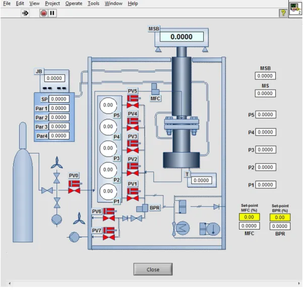
Figure 3.1 - Schematic diagram of the experimental set-up for adsorption

measurements. Labeling is as follows: BPR, back-pressure regulator; MFC, mass-flow

controller; MSB, magnetic suspension balance; P1-P5, pressure transducers; Pt 1 0 0,

thermocouples; JB, JULABO bath; PV0-7, pneumatic valves from Swagelok, 1/8 tube

diameter from Swagelok, vacuum assured by BOB Edwards vacuum pump. ... 12

Figure 4.1 - Routine for acquisition and recording of data from the magnetic suspension

balance. ... 18

Figure 4.2 - Representation of a parallel port. ... 19

Figure 4.3 - Routine that sends the commands to the controller unit of the balance. .. 21

Figure 4.4 - Algorithm to control the balance... 22

Figure 4.5 - Algorithm of communication with the Sartorius balance. ... 23

Figure 4.6 - RS232 cable pin-out for communication between the Sartorius balance and

the computer... 24

Figure 4.7 - RS232 cable pin-out for communication between the MKS pressure sensor

and the computer... 25

Figure 4.8 - Algorithm to read the pressure from the MKS pressure sensor. ... 26

Figure 4.9 - RS232 cable pin-out for communication between the JULABO thermostatic

bath and the computer... 27

Figure 4.10 - Algorithm to communicate with the Julabo thermostatic bath. ... 29

Figure 4.11 - Old interface with just one window... 30

Figure 4.13 - Settings of Interface, where is configured the input channels... 32

Figure 4.14 - Control input variables. ... 33

Figure 4.15 - Settings of Interface, where it’s configured the output channels... 34

Figure 4.16 - Control output variables. ... 35

Figure 4.17 - Process interface. ... 36

Figure 4.18 - Isotherm measuring interface... 37

Figure 4.19 - Buttons of Isotherm measuring interface. ... 37

Figure 4.20 - Monitoring interface... 38

Figure 4.21 - Experiment annotation interface. ... 39

v  

Index of Tables

Table 1.1 - Parameters estimated by calibration of the empty system. ...9

Table 2.1 - Correspondence between the controller and the board PCI 6023E. ...20

Table 2.2 - Correspondence between the Sartorius balance and the computer...24

Table 2.3 - Correspondence between the MKS and the computer. ...25

Table 2.4 - Correspondence between the JULABO and the computer...27

Table 4.5 - Isotherm data of CO2 on Zeolite 5A and MIL-53(Al) samples, for 30ºC...40

Table 4.6 - Isotherm data of CO2 on Zeolite 5A and MIL53(Al) samples, for 50ºC. ...41

vii  

Abbreviations

BPR – Back Pressure Regulator

CTS – Clear to Send

GND – Ground

IUPAC – International Union of Pure and Applied Chemistry

JB – Julabo Bath

MFC – Mass flow controller

MOF – Metal-organic framework

MP1 – Measuring Point 1

MP2 – Measuring Point 2

MS – Mass spectrometer

MSB – Magnetic Suspension Balance

PSA – Pressure Swing Adsorption

RTS – Request to send

ZP – Zero Point

ix  

Symbology

mh -Mass of the cell

ms -Mass of the adsorbent sample

ρg -Density of the bulk gas at the equilibrium P and T

ρh - Density of the cell

ρs -Density of the adsorbent sample

qex -Specific excess adsorption

Vh - Volume of all moving parts present in the measuring cell

Vp - Total pore volume

Vs - Specific adsorbent volume impenetrable to the adsorbate

w - Weigh

wZP - Measured weight in ZP

wMP1 - Measured weight in MP1

wMP2 - Measured weight in MP2

1  

Chapter 1 – Introduction

1.1. Motivation

Adsorption processes have been largely used in chemical industry and are of great technological importance, being actually a big area in expansion with the development of new processes.

Thus, some adsorbents are used on a large scale as desiccants, catalysts or catalyst supports; others are used for the separation of gases, the purification of liquids, pollution control or for respiratory protection. In addition, adsorption phenomena play a vital role in many solid state reactions and biological mechanisms (Rouquerol, Rouquerol et al. 1999). Examples of adsorption separation processes are oxygen/nitrogen separation from air (Etéve, Hay et al. 1993) and biogas upgrading (Grande 2011).

Moreover, during the last years new classes of solid adsorbents have been developed, such as activated carbon fibres and carbon molecular sieves, fullerenes and heterofullerenes, microporous glasses and nanoporous - both carbonaceous and inorganic - materials. Nanostructured solids are very popular in science and technology and have gained extreme interest due to their sorption, catalytic, magnetic, optical and thermal properties (Dąbrowski 2001).

Therefore, is necessary the development of new methods of monitoring, control and optimization of adsorption processes.

1.2. Framing Work

This thesis follows a set of work already realized in a system for obtaining adsorption isotherms, located in the Department of Chemistry at FCT-UNL. The main objective is the development of a new interface in LabVIEW for acquisition, control and monitoring of adsorption isotherms.

(Sousa 2009) developed a new interface for the magnetic suspension balance used in the installation but with the gain of a new state of the balance, it was necessary to develop a new interface.

measurement of adsorption isotherms.

3  

Chapter 2 - Bibliographic Review

Adsorption is a surface phenomenon that occurs when a solid surface is exposed to a fluid.

All adsorption separation processes involve two principal steps: (1) adsorption, during which the preferentially adsorbed species are picked up from the feed; (2) regeneration or desorption, during which these species are removed from the adsorbent, thus “regenerating” the adsorbent for use in the next cycle (Ruthven, Farooq et al. 1938).

The solid phase on which adsorption occurs is called the adsorbent and the group of molecules that are adsorbed on the surface of the solid material is called the adsorbate.

The adsorbents used in this study are zeolite 5A and MIL-53(Al).

MIL-53(Al), nanoporous aluminum terephthalate, is a MOF material. MOF materials (metal organic frameworks) are a class of structured nanoporous materials. Due to their high porosity, high adsorption capacity, and thermal stability, these materials have shown great potential for applications in gas storage, gas separation, catalysis, and allied fields. MIL-53(Al) is from a very interesting class of MOF materials because they not only adsorb large amount of gases, such as H2, CO2, and light alkanes, but also exhibit exceptional flexibility by undergoing

Zeolite 5A is a Na+ and Ca2+ exchanged zeolite type A with 1:1 Si:Al ratio. It is crystalline and highly porous, with an internal network of angstrom-sized pores (4.3 Å), similar to the dimensions of small molecules (Ghosh, Ma et al. 2013).

Experimental adsorption isotherms recorded in the literature, measured on a wide variety of gas-solid systems, have a wide variety of forms. Nevertheless, the majority of these isotherms, which result from physical adsorption, may conveniently be grouped into six classes in the IUPAC classification as shown in the Figure 2.2 (Rouquerol, Rouquerol et al. 1999).

(Rouquerol, Rouquerol et al. 1999).

The Type I isotherm is characterized by the existence of a plateau, which is visible from relatively low pressures, which corresponds to adsorption mechanism in micropores. Thus the plateau corresponds to complete filling and from the height of the plateau is possible to determine the volume of micropores (Figueiredo and Ribeiro 2007)

5  

The two methods, normally, used to determinate adsorption isotherms are volumetric and gravimetric measurements.

Volumetry, also called as Manometry, is the oldest method to investigate sorption of gases in solids (Keller and Staudt 2005). This method is based on the measurement of the gas pressure in a calibrated, constant volume, at a known temperature (Rouquerol, Rouquerol et al. 1999);(Keller and Staudt 2005).

Volumetric gas adsorption instruments are quite easy to be used and automated but there are some disadvantages associated to this method, as the necessity of large amounts of sorbent material and the difficulty to approach the equilibrium.

The gravimetric technique is more recent and known to be much more accurate than the volumetric measuring method.

This technique not only is more accurate but it also allows to check whether an adsorption system actually has reached its equilibrium state and to give information about the kinetics of the adsorption process.

Also for highly sensitive microbalances, only tiny amounts of sorbent materials are needed to measure gas adsorption equilibria (Keller and Staudt 2005).

Figure 2.3 - Gravimetric measurements under controlled environments. Comparison of conventional

instrument (left) and magnetic suspension balance (right). UHV means Ultra-high vacuum (Dreisbach and

Lösch 2000).

In this particular case, it’s used a gravimetric method by using a high-pressure magnetic suspension balance (MSB), model ISOSORP 2000, from Rubotherm (GmbH).

The magnetic suspension balance allows the change in force and mass which act on samples under controlled environments (pressure, temperature, corrosive gases or fluids) (Manual 2000).

As shown, in the figure 4, the balance has four possible states that are used to perform the mass gain measurements:

• OFF: the magnetic suspension is not attracted by the electromagnet and so lays down on the coupling house.

• Zero point: the permanent magnet alone is in a freely suspended state, allowing the balance to be tared and calibrated.

• Measuring point 1: the first sample is lifted up and its mass is weighed.

7  

2011).

The existence of MP2 allows simultaneous sorption and density measuring as well as comparing measurements of two samples. To calculate the density, it’s necessary to weigh a titanium sinker with a calibrated volume as the second sample.

The weight, w, obtained by the balance, as a result of the force that acts on the sample is given by:

(1)

With,

• mh and ρh the mass and density of the cell, respectively;

• ms and ρs are the mass and density of the adsorbent sample, respectively; •ρg is the density of the bulk gas at the equilibrium P and T;

The cell container mass and volume are measured independently with a gas, usually helium or nitrogen, before sample loading. Thus, the blank experiments with the empty measuring cell give its mass and density from the intercept and slope of the linear decrease of apparent weight with gas density,

(2)

The values of mh and ρh were estimated by a unique calibration of the empty system

(without sample) for each cell with helium at 20,63ºC.

9  

state system.

The linear fitting provided the values of mh and ρh, for the two measurements.

Table 1.1 - Parameters estimated by calibration of the empty system.

Cell mh (g) ρh (g/cm 3

)

First 5.5743 7.96

Second 6.4118 8.01

In the case of a gravimetric measurement, the net amount adsorbed on a dry basis, expressed in moles of CO2 adsorbed per gram of dried sample, is given by

(3)

Where, Vh is the volume of all moving parts present in the measuring cell (such as the

holding basket) that are subjected to the buoyancy force exerted by the gas. However, adsorption measurements are invariably reported in terms of excess adsorption, qex, which is

that would be present in the same system, at the same (P, T), if the gas did not adsorb into the solid. The excess amount, qex, is related to qnet through

(4)

where, ρs is the skeletal (or structural) density of the adsorbent. The absolute adsorption

(or total amount adsorbed) is related with qex and qnet by

(5)

where, Vp is the accessible total pore volume of the adsorbent and Vs = 1/ρs is the

specific adsorbent volume impenetrable to the adsorbate.

11  

Chapter 3 – Experimental Procedure

3.1.

Materials

The adsorbents used in this study are Zeolite 5A and MIL-53(Al). MIL-53(Al) has a surface area of 1100-1500 m2/g and its structure is stable up to 773 K (Lyubchyk, Esteves et al. 2011). Zeolite 5A has a surface area of 571 m2/g (Liu, Grande et al. 2011; Zhen Liu 2011).

The crystalline structure of MIL-53(Al) powder was synthesized by BASF under the trade-mark Basolite A100 and Zeolite 5A spheres were synthesized by (60-80 mesh) Supelco.

3.2. Adsorption experiments

The adsorption experiments were carried out using a closed-loop gravimetry. The main piece of equipment used in the experiments is a high-pressure magnetic suspension balance (MSB), model ISOSORP 2000, from Rubotherm (GmbH), with automated online data acquisition of temperature, pressure, and sample weigh.

The advantage of the MSB is the possibility of accurately weighing samples contactlessly under nearly all environments. Instead of hanging directly at the balance, the sample is coupled to a suspension magnet, achieving a constant vertical position in a closed measuring cell. The MSB has a resolution of 0.01 mg, an uncertainty ≤ 0.002%, and a reproducibility ≤ 0.03 mg, for a maximum load of 25 g.

The conditions that can be imposed on the measuring chamber are limited to 100ºC and 150 bar. A mass-flow meter/controller (MFC) from HASTINGS (0.1-10 SLPM N2), with a 1% FS (full-scale) accuracy, can be coupled to the feed line. The temperature is measured and controlled using four-wire Pt 100 probe and one thermostatic bath from JULABO; the cell temperature is kept within ± 0.1 K of the set-point. A Bronkhrost back-pressure regulator (BPR), with 0.5% FS accuracy, can be coupled to the outlet line to control the pressure in the chamber for the continuous-flow experiments; the controllable pressure range is 0-150 bar, at T < 373 K. Five transducers can be employed to accurately measure different pressure ranges: MKS Barathon 627D for 0-1 bar with 0.15% of reading; OMEGADYNE for 0-10 bar with 0.05% FS accuracy; OMEGADYNE for 0-20 bar with 0.05% FS accuracy; OMEGADYNE for 0-35 bar with 0.05% FS accuracy; OMEGADYNE for 0-69/138/207 bar with 0.15% FS accuracy.

Figure 3.1 - Schematic diagram of the experimental set-up for adsorption measurements. Labeling

is as follows: BPR, back-pressure regulator; MFC, mass-flow controller; MSB, magnetic suspension

balance; P1-P5, pressure transducers; Pt 1 0 0, thermocouples; JB, JULABO bath; PV0-7, pneumatic

valves from Swagelok, 1/8 tube diameter from Swagelok, vacuum assured by BOB Edwards vacuum

pump.

13  

15  

Chapter 4 – Development of interface

4.1.

Acquisition and Process data

The software we are developing has 3 main objectives:

- To automate the monitoring of the main variables, such as pressure and temperature; - To automate the control of the temperature and pressure of the MSB;

- To automate the process of measuring adsorption isotherms.

The acquisition of data from the micro-balance is done continuously, this means that it is continually reading the weight to obtain an isotherm, are needed several equilibrium points for different gas pressures at a constant temperature.

Figure 8 shows the algorithm of the routine of acquiring and registration of data. As can be seen in the mentioned figure, the algorithm for measuring isotherms starts by fixing a certain pressure and this is the pressure that we want for measuring one point of the adsorption isotherm. It is necessary to wait for the equilibrium, so that we can measure the amount of gas adsorbed. The program plots and saves intermediate adsorption measuring points, allowing to check whether an adsorption system actually has reached its equilibrium state.

The process of measuring isotherm points starts with the balance controller in OFF position. When the controller is in OFF position, the only option is to change it to Zero Point position (ZP). As it was said in the introduction, in this Zero Point position the permanent magnet alone is in a freely suspended state, allowing the balance to be tared and calibrated.

In this routine we use equation 8 to correct the measured weight values, allowing the adjustment of any external or internal disturbances that affect the stability of the Zero Point. To correct the measuring data even with small changes, zero points are taken within a relative short interval.

The slope between two following zero points it’s calculated by

(8)

With wZP(t) being the obtained weight in zero point for the instant t; wZP(t-F) being the

Normally, is measured just one point but to make this routine as general as possible, it’s permitted to measure various points and to calculate an average in the different states of the balance.

When the balance controller is in ZP position, is possible to change it to OFF or MP1.

In Measuring Point 1, the first sample is lifted up and its mass is weighed. Using this slope it directly calculates the corrected value for each measuring point 1 taken between these two zero points with

(9)

where wMP1c is the corrected weigh for the instant i between t-F and t and wMP1 the

measured weight for the instant i (MessPro).

Usually the ZP is tared to zero un order to eliminate possible electronic drifts in the balance controller unit.

The corrected weight difference listed in the data-file results of the corrected absolute weight minus the reference value:

(10)

When the balance controller is in MP1 position, it’s possible to change it to ZP or MP2. In the Measuring point 2, the second sample is raised with the first sample and both masses are weighed together (MessPro ; JULABO 2011).

To calculate the absolute weight-value of MP2 the relevant absolute MP1-value will be subtracted from the recorded MP2-value.

(11)

In MP2 the balance can either measure the weight of the sinker or it can measure the weight of the second adsorbent under study.

17  

With MP2, is not only possible to measure two different samples at the same time but it’s also possible the measurement of the density if a titanium sinker is weighed as the second sample (g/cm3):

(13)

When the balance controller is in MP2 position, the only option is to change it to MP1 position, after which the user adopts the ZP position to further increase (or decrease) the system pressure to proceed with the adsorption equilibria measurements.

Along with the measurement of the weight, the temperature is monitored and controlled, using a thermostatic bath from Julabo.

Some variables are defined by the user, such as the number of points in Zero Point position (nr ZP points), the interval time necessary to stabilize the balance before measuring the value of ZP (ΔZP), the number of points in Measuring Point 1 position (nr MP1 points), the interval time necessary to stabilize the balance before measuring the value of MP1 (ΔMP1), the number of points in Measuring Point 2 position, the interval time necessary to stabilize the balance before measuring the value of MP2 (ΔMP2), the minimum slope from which it is considered that the system is stable in Measuring Point 1 position (ΔslopeMP1), the minimum slope from which it is considered that the system is stable in Measuring Point 2 position (ΔslopeMP2), in the settings of the interface of isotherms measurement.

19  

4.1.1. Communication with the balance controller

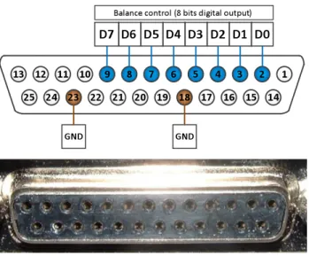
Previously, the communication between the control system of the balance and software was made using a port LPT1, parallel port (typically used for printers).

However, recent computers don’t have LPT1 port available. Figure 9 shows that the LPT1 digital communication is done using 8 bits digital port. Therefore, it’s possible to replace the communication using a board with 8 bits digital output port, in this case a National Instruments PCI 6023E internal board.

Table 2 shows the correspondence between the 25 pin controller output port and the board PCI 6023E. The table also shows the colors of the cables used in the connection.

Table 2.1 - Correspondence between the controller and the board PCI 6023E.

Pin (LPT1) Pin (PCI 6023E) Digital Output Cable Colour

2 52 D0 Blue

3 17 D1 Red

4 49 D2 Orange

6 19 D4 Grey

7 51 D5 Green

9 48 D7 Yellow

18 12 Ground Black

23 13 Ground Brown

Figure 10 shows the 8 bits corresponding to the different commands we can send to the balance control. OFF(0), ZP (32), MP1 (160), MP2 (176) are the most important commands.

The other commands correspond, normally, to error situations and this means that we are not interested in writing these commands to the digital port.

21  

Figure 4.3 - Routine that sends the commands to the controller unit of the balance.

4.1.2. Communication with the Sartorius balance

To determinate the isotherm, it is necessary to measure the weight in MPi (i=1, 2) or to

tare the balance. Therefore the communication with the Sartorious balance is very important.

23  

Table  2.2  -­‐  Correspondence between the Sartorius balance and the computer.  

Balance (25-pin male)

Computer (9-pin female)

Pin 2

Data

Output

(TxD)

Black

Out

Pin 2

Receive

Data

(RxD)

In

Pin 3

Data

Input

(RxD)

Brown

In

Pin 3

Transmit

Data

(TxD)

Out

Pin 4

Pin 14

Internal

Ground

(GND)

Green

--

Pin 5

Ground

(GND)

--

Pin 5

Clear to

Send

(CTS)

Yellow

In

Pin 4

Data

Terminal

Ready

(DTR)

Out

Pin 6

Data Set

Ready

(DSR)

In

Pin 20

Data

Terminal

Ready

(DTR)

Red

out

25  

4.1.3. Communication with the MKS pressure sensor

To measure pressures in the range of 0 to 1 bar is used a MKS sensor. This sensor communicates with the computer using the protocol RS232 with 9600 baud rate, 7 data bits, odd parity and 1 stop bits. To start the communication with the sensor is necessary to write “char31 + Char25” in the serial port. To read a new pressure value we need to write “Carriage return + line feed” to the serial port.

The connection between the sensor and the 9-pin serial port of the computer is standard, as it’s shown in Table 4 and Figure 14.

Figure 4.7 - RS232 cable pin-out for communication between the MKS pressure sensor and the computer.

Table 2.3 - Correspondence between the MKS and the computer.

MKS (25-pin male)

Computer (9-pin female)

Pin 2

Data

Input

(RxD)

Red

In

Pin 3

Transmit

Data

(TxD)

Out

Pin 3

Data

Output

(TxD)

Green

Out

Pin 2

Receive

Data

(RxD)

In

Pin 5

Ground

(GND)

Black

--

Pin 5

Ground

(GND)

27  

4.1.4. Communication with JULABO thermostatic bath

The communication with JULABO thermostatic bath is made using the interface RS232, with baud rate of 4800, 7 data bits, even parity and 1 stop bits.

The connection between the JULABO thermostatic Bath and the 9-pin serial port of the computer is shown in Table 4 and Figure 16.

Figure 4.9 - RS232 cable pin-out for communication between the JULABO thermostatic bath and the computer.

Table 2.4 - Correspondence between the JULABO and the computer.

Julabo (25-pin male)

Computer (9-pin female)

Pin 2

Data

Input

(RxD)

Red

In

Pin 3

Transmit

Data

(TxD)

Out

Pin 3

Data

Output

(TxD)

Green

Out

Pin 2

Receive

Data

(RxD)

In

Pin 5

Ground

(GND)

Black

In

Pin 5

Ground

(GND)

--

Pin 7

Request

to Send

(RTS)

Blue

out

Pin 8

Clear to

Send

(CTS)

In

Pin 8

Clear to

Send

(CTS)

Yellow

In

Pin 7

Request

to send

(RTS)

There are two types of commands: output commands and input commands.

Figure 17 shows the algorithm to communicate with the JULABO thermostatic bath. In this communication between the JULABO thermostatic bath and the computer, are used several commands, specially, output commands.

Output commands

Some of the most utilized output commands are those that set working temperatures.

The Julabo can save 3 setpoints using the commands: "Out_sp_00\ sX.XX\r" to change the value of the setpoint 0; "Out_sp_01\sX.XX\r" to change the value of the setpoint 1 and “Out_sp_02\sX.XX\r" to change the value of the setpoint 2.

To exemplify, when we write on the door "out_sp_00\s16.00\r", “\s” means space and “\r” means return, and the command writes in Julabo to put the Setpoint between 0 to 6.0 º C. If it’s written "Out_sp_01\s12.00\r", the setpoint it’s defined between 1-12 º C and if is written "Out_sp_02\s18.00\r", the setpoint is defined between 2-18 º C.

The command "out_mode_01i\r" , where i = 0,1,2 , allows the selection of the active setpoint. For example, the command "out_mode_010\r" activates the setpoint 0 (this means, the system controls the bath to 6 º C temperature). The command "out_mode_011\r" selects the setpoint 1 and "out_mode_012\r" selects the setpoint 2.

The command "out_mode_04\s0\r " allows the selection of the internal temperature sensor as a control variable and the command "out_mode_04\s1\r" allows the selection of the external sensor as a control variable to monitor the temperature in the balance.

To stop the recirculating bath, it’s used the command "out_mode_05\s0\r" and to reconnect this same command, it’s used "out_mode_05\s1\r".

(JULABO 2011) lists other output commands that can be used but are not relevant in this work.

Input commands

29  

Is possible to make an inquire with the "status" command. In response to this command, the system sends a status message or an error message. If there is no error, the normal response to this command is "Circulator in remote control mode", if the system is in manual control, the answer will be "Circulator in keypad control mode". If no error the system responds with an error message, for example, "Low liquid level alarm". The device manual lists all the error messages.

4.2. Interface

Previously, the software only had one window to monitoring, control and automate the process. Modify the program and to reuse the source code was very complicated and time consuming.

This thesis began with the development of the old software (Figure 18) in order to maximize the reuse of source code, the implementation of new processes, and changing the graphical interface.

In figure 19, is represented the new main interface of the program, that only has one icon bar to call the other modules that are now independent from each other, allowing us to build different interfaces to control different processes.

31  

In this software, the objective is to control the Magnetic Suspension Balance but is possible to use the same interface to control other programs if some of the routines are changed. The routines of monitoring, experimental annotation, for example, are the same.

Besides the horizontal bar, the menus allow the interaction with the different modules.

The File Menu has 5 main inputs: Settings, Control, Export, Exit and Quit. Control is still not fully implemented and the objective is to permit defining controllers (for example, PI, P, PID, MPC, etc.), what the controller parameters are and what are the manipulated variables and measured variables. Export, as the name says, allows exporting the data to a text file or a spreadsheet file, as excel, for example. The difference between exit and quit is that the exit button leaves the program but saves the last configurations of the system and the button quit aborts the experiment, leaving the process without saving it.

The Analyze Menu allows the access to the history of the process. There are two interfaces that permit to see the process history, an interface with just one window and an interface with four windows.

The settings in the File Menu permit to select the variable name and the driver of communication that is used to acquire data.

As  it  was  stated  before,  there  are  input  channels  

(read)  and  output  channels  (write)  and  they  are  defined  in  the  Settings.

In figure 20, is shown the settings window where is possible to configure the input channels.

33  

First, it’s necessary to define the input channels and their drivers. Then in the Control section, Control Input Variables, is possible to select the drivers that were previously defined in the input channels, to read and represent in the graphic. This means, that we associate the input channels that correspond to the process inputs that are being controlled, monitored and automated.

In figure 21, it’s shown the Control Section, when the input channels are associated.

In figure 22, it’s shown the settings of the output channels.

Is necessary to do the same definition procedure as it was done for the input channels. First, the channels are defined and then in the Control section, Control Output Variables, is possible to activate the drivers that were previously defined in the output channels.

In the figure 22, Driver is the driver used for communication between the instrument and Laptop Computer. Each device has a driver and examples of drivers are described in the previous chapter, for example, communication with the scale, with the Julabo communication, communication with the MKS, etc.

35  

4.2.1. Interface modules

As it was said, earlier in this chapter, there are 5 interface models, being Control still incomplete.

In Figure 24 it’s represented the Process module interface and as is possible to see, the Process interface has 8 digital outputs (with OFF and ON symbols being represented in red and green, respectively), 2 Analog outputs and 8 Analog inputs. The balance control has 8 digital channels but it is not implemented in this interface, it is only in the isotherm measuring interface.

In figure 25, is possible to see the new isotherm measuring interface, where is implemented the algorithm shown in the chapter 4.1.

37  

The Isotherm measuring interface shows the values of ZP, MP1, MP2, the respective isotherm and the reading weight on the top.

The three button in blue represented in Figure 25 are Tare button, Read button and Calibration button, respectively. Tare button is need to tare de balance in manual mode, the R button reads in manual mode and Cal button proceeds the calibration of the balance. Above these three buttons, it is indicated the instantaneous reading of the weights. This buttons only work in manual mode.

Figure 4.19 - Buttons of Isotherm measuring interface.

When Run, represented in Figure 26, starts, the buttons of manual control are disabled. In that figure there are some other buttons represented as the settings button, the data table button (results shown in a table, rather than graphic), X button to abort the automatic mode.

In Figure 27, is shown the monitoring interface, where it’s possible to choose the graphics and the signal that we want in each graphic, being possible to associate a color.

Figure 28, represents the Experiment annotation interface.

39  

4.3.

Experimental Validation

The adsorption isotherms data represented in tables 2-4 were obtained at three different temperatures: 30ºC, 50ºC and 80ºC. Each point of the isotherm is determined by the weight gain in the sample for a specific pressure.

After the determination of all points of the isotherms, it was possible to determinate qex,

qnet and qtotal, using the Eqs. 3, 4 and 5.

In Figures 29, 30 and 31, is possible to see the adsorption isotherms for CO2 on Zeolite

5Aand MIL-53(Al)

Table 4.5 - Isotherm data of CO2 on Zeolite 5A and MIL-53(Al) samples, for 30ºC.

Z5A MIL-53(Al)

MP1 MP2 P T qnet qex qt qnet qex qt

41  

Table 4.6 - Isotherm data of CO2 on Zeolite 5A and MIL53(Al) samples, for 50ºC.

MP1 MP2 P T qnet qex qt qnet qex qt

g g bar ºC mol/kg mol/kg mol/kg mol/kg mol/kg mol/kg 6,071 6,723 0,000 50,39 0,000 0,000 0,000 0,000 0,000 0,000 6,073 6,723 0,002 49,97 0,082 0,082 0,082 0,032 0,032 0,032 6,078 6,724 0,013 50,08 0,325 0,326 0,326 0,085 0,085 0,085 6,089 6,726 0,044 50,03 0,822 0,823 0,824 0,232 0,233 0,234 6,101 6,729 0,095 50,06 1,375 1,378 1,379 0,455 0,457 0,459 6,124 6,736 0,374 50,06 2,416 2,426 2,430 0,976 0,982 0,990 6,133 6,740 0,946 50,07 2,871 2,896 2,907 1,385 1,402 1,421 6,140 6,747 3,193 50,04 3,290 3,377 3,413 2,054 2,111 2,178 6,140 6,748 4,558 50,08 3,387 3,512 3,564 2,331 2,412 2,509 6,139 6,750 6,573 50,03 3,468 3,650 3,725 2,667 2,785 2,926 6,138 6,751 8,526 50,04 3,514 3,752 3,850 2,928 3,082 3,266 6,137 6,751 9,764 50,03 3,535 3,808 3,921 3,082 3,259 3,471 6,135 6,751 11,976 50,05 3,560 3,898 4,038 3,303 3,522 3,785 6,131 6,750 15,052 50,01 3,570 4,001 4,179 3,524 3,804 4,139 6,128 6,748 17,492 49,99 3,564 4,070 4,280 3,661 3,990 4,383 6,124 6,746 19,981 50,01 3,563 4,148 4,390 3,803 4,183 4,637 6,114 6,738 26,086 50,02 3,502 4,287 4,613 3,978 4,488 5,098 6,102 6,728 32,926 50,03 3,404 4,430 4,856 4,081 4,747 5,544 6,122 6,746 21,400 50,01 3,556 4,186 4,447 3,941 4,350 4,840 6,133 6,753 13,496 50,02 3,587 3,970 4,129 3,591 3,840 4,138 6,139 6,742 1,976 49,97 3,201 3,254 3,276 1,613 1,648 1,689 6,131 6,733 0,685 50,06 2,787 2,805 2,813 0,849 0,861 0,876 6,099 6,725 0,041 50,02 1,278 1,279 1,279 0,189 0,190 0,191 6,079 6,724 0,003 49,99 0,355 0,355 0,355 0,071 0,071 0,071 6,077 6,723 0,000 50,13 0,242 0,242 0,242 0,035 0,035 0,035

Table 4.7 - Isotherm data of CO2 on Zeolite 5A and MIL53(Al) samples, for 80ºC.

Z5A MIL53(Al)

MP1 MP2 P T qnet qex qt qnet qex qt

6,165 6,738 13,155 79,980 3,096 3,433 3,573 2,511 2,729 2,991 6,170 6,736 4,946 79,900 2,925 3,048 3,099 1,631 1,712 1,808 6,169 6,734 3,511 80,090 2,814 2,901 2,937 1,333 1,389 1,457 6,162 6,728 1,468 79,990 2,428 2,464 2,480 0,729 0,752 0,781 6,131 6,721 0,129 79,930 1,048 1,051 1,053 0,098 0,100 0,103 6,117 6,720 0,028 80,020 0,425 0,426 0,426 0,029 0,029 0,030 6,110 6,720 0,000 79,900 0,146 0,146 0,146 0,006 0,006 0,006

0   1   2   3   4   5   6   7  

0   5   10   15   20   25   30   35  

q t (mol /k g) P (bar) 30 ºC 50 ºC 80 ºC

0   1   2   3   4   5   6   7  

43  

From the results, it can be said that the interface developed is acquiring the values of the weight correctly and applying well the correction of the zero point, allowing the user to simplify the process of determining adsorption isotherms.

45  

Chapter 5 – Conclusion and Future Work

5.1.

Conclusion

In this work, the objective was to build an interface with five separated modules. It were developed two modules, the module of control of the MSB and the isotherm measuring module.

The developed interface permits the acquisition of the weight obtained by the balance and the control of the measuring positions of the balance. It was possible to apply a correction algorithm through the deviations of the zero point and, consequently, to correct the values of the obtained weight. All the acquisition is automated, existing an algorithm that synchronizes it in real-time, controlling the balance positions and obtaining the respective values of weight.

From the results, it can be confirmed that the interface developed is acquiring the values of the weight correctly and applying well the correction of the zero point, allowing the user to simplify the process of determining adsorption isotherms.

5.2.

Future Work

After this work, the installation showed a significant progress in motoring and control. However, the interface is still incomplete and there are still improvements to do for the complete automation of the installation.

Suggestions for future work to continue improving the interface:

- To allow the user to select the isotherm model and adjust the parameters of the isotherm in real time or offline.

- To connect the balance to the Mass Spectrometer (MS), so we can work with mixtures;

- To end and improve the code interface that has been done, as it’s still very raw and specifically directed to this concrete process of measuring gas isotherms. For example the process control routine is integrated into the isotherm measuring interface and not in the process control interface.

- To implement an easy way to associate controllers to the process, choosing the manipulated variables, measured variables and set points (controllers like Proportional (P),

Proportional and Integral (PI), Proportional + Integral + Derivative (PID), Model Process Control

(MPC);

- To better define how it is the communication between the different modules in order to allow the software to be used in order processes.

- To allow the use of external software channels, for example, gPROMS, AMPL, MATLAB or even channels define by a DLL, so we can use fortran, c, c++ code to program a driver or a controller.

- To allow the addition of auxiliary channels that operate on physical channels of acquisition, for example, a channel that is the derivative of another channel or the result of another mathematical operation including software filters.

- To allow the user to define tasks which will be done in sequence or in parallel, so the user can automate sequential processes.

47  

Chapter 6 – Bibliography

[1]. Dąbrowski, A. (2001). "Adsorption — from theory to practice." Advances in Colloid and Interface Science 93(1–3): 135-224.

[2]. Dreisbach, F. and H. W. Lösch (2000). "Magnetic Suspension Balance for Simultaneous Measurement of a Sample and the density of the measuring fluid."

[3]. Esteves, I. A. A. C., M. S. S. Lopes, et al. (2008). "Adsorption of natural gas and biogas components on activated carbon." Separation and Purification Technology 62(2): 281-296.

[4]. Etéve, S., L. Hay, et al. (1993). Method for Producing Oxygen by Adsorption Separation from Air. S. a. p. l. E. e. l. E. d. P. G. C. L'Air Liquide, Paris, France. France. 5,223,004.

[5]. Figueiredo, J. L. and F. R. Ribeiro (2007). Catálise Heterogénea, Fundação Calouste Gulbenkian.

[6]. Ghosh, A., L. Ma, et al. (2013). "Zeolite molecular sieve 5A acts as a reinforcing filler, altering the morphological, mechanical, and thermal properties of chitosan." Journal of Materials Science 48(11): 3926-3935.

[7]. Grande, C. A. (2011). "Biogas Upgrading by Pressure Swing Adsorption." SINTEF Materials and Chemistry, Oslo Norway.

[8]. JULABO (2011). Operating Manual, JULABO Labortechnik GmbH.

[9]. Keller, J. and R. Staudt (2005). Gas Adsorption Equilibria.

Liu, Z., C. A. Grande, et al. (2011). "Adsorption and Desorption of Carbon Dioxide and Nitrogen on Zeolite 5A." Separation Science and Technology 46(3): 434-451.

[10]. Lyubchyk, A., I. A. A. C. Esteves, et al. (2011). "Experimental and Theoretical Studies of Supercritical Methane Adsorption in the MIL-53(Al) Metal Organic Framework." Journal of Physical Chemistry C 115(42): 20628-20638.

[11]. Manual, R. (2000). "The New Sorption Suspension Balance."

[12]. MessPro, U. s. M. f.

[13]. Ramsahye, N. A., G. Maurin, et al. (2008). "Probing the Adsorption Sites for CO2 in Metal Organic Frameworks Materials MIL-53 (Al, Cr) and MIL-47 (V) by Density Functional Theory." J. Phys. Chem. C, Institut Charles Gerhardt Montpellier.

[14]. Rouquerol, J., F. Rouquerol, et al. (1999). Adsorption by Powders and Porous Solids - Principles, Methodology and Applications, Academic Press.

[15]. Ruthven, D. M., S. Farooq, et al. (1938). Pressure Swing Adsorption.

[16]. Saha, D., Z. Bao, et al. (2010). "Adsorption of CO2, CH4, N2O, and N2 on MOF-5, MOF-177, and Zeolite 5A." Chemical Engineering Department, New Mexico State University, Las Cruces, New Mexico

[18]. Sousa, G. M. R. P. L. (2009). Implementação de Sistemas para Controlo e Monitorização de Equilíbrio, Cinética e Dinâmica de Adsorção.