Are electricity ordinary and special regimes driving economic activity?

UNIVERSIDADE DA BEIRA INTERIOR

Ciências Sociais e Humanas

Are electricity ordinary and special regimes

driving economic activity? The Spanish evidence

Sónia Cristina Almeida Neves

Dissertação para obtenção do Grau de Mestre em

Economia

(2º ciclo de estudos)

Orientador: Prof. Doutor António Manuel Cardoso Marques

iii

Acknowledgments

This important stage of my life would not have been possible without the support and comprehension of multiple persons to whom I want to express my heartfelt acknowledgement.

First, I want to like to thank my parents, brother and my grandmother, for all the support, incentive and understanding. Secondly, I would like express my gratitude to my supervisor, Doctor Professor António Cardoso Marques for his immeasurable guidance, unconditional support and friendship. I would also like to thank Doctor Professor José Alberto Fuinhas for his assistance, support and friendship. Fourth would like to thank my boyfriend, Raul Nunes, for his support, patience and comprehension he had to have over the recent times. To my housemates, André Nunes, Carla Tomás and Diogo Pereira, I am grateful for all the patience that they had to have in the worst times, for all the help and unconditional support. Finally, and not least, I would like to thank all the friends I made in Covilhã who accompanied me in these important years of my life, especially Joana Almeida.

v

Resumo

A presente dissertação estuda a interação entre fontes de geração de eletricidade através da produção sob regime especial e sob regime ordinário e a sua relação com a atividade económica. O estudo utiliza dados mensais de Janeiro de 2003 até Setembro de 2014. O teste de causalidade Toda-Yamamoto foi executado para averiguar quais as relações de causalidade existentes entre as variáveis. A metodologia ARDL bounds test permitiu capturar os efeitos de curto e de longo prazo em separado. Globalmente, os resultados das causalidades revelam grande consistência quando comparados com os resultados da metodologia ARDL. Os resultados sugerem a existência de uma causalidade unidirecional da produção de eletricidade em regime ordinário para o regime especial. Analisando o tradicional nexus pode-se concluir que a hipótepode-se de feedback é verificada entre o regime ordinário e a atividade económica. Por outro lado, verifica-se também que o regime especial é um entrave ao crescimento da atividade económica.

Palavras-chave

ARDL bounds test, nexus eletricidade-crescimento, Regime Ordinário e Especial, Sistema elétrico Espanhol, Teste de causalidade Toda-Yamamoto

vi

Resumo Alargado

No atual contexto Europeu, a diversificação do mix de energia é uma prioridade, prevista na diretiva comunitária directive 2009/28CE (European Commission, 2009). A tendência de investimento em geração de eletricidade renovável tem como consequência, como por exemplo, a acomodação das diferentes fontes de produção elétrica no sistema.

O nexus consumo de energia/eletricidade tem sido bastante debatido na literatura e consiste na análise da relação causal entre as variáveis consumo de energia e crescimento económico. Nesse sentido foram definidas quatro hipóteses explicativas para a interação entre as variáveis. Segundo a hipótese crescimento, um aumento do consumo de energia gera um aumento do crescimento económico, ou seja, existe uma relação unidirecional de consumo de energia para crescimento económico. De acordo com a hipótese de conservação, pode ser observável crescimento económico sem ser necessário a existência de uma unidade adicional de consumo de energia, quer isto dizer que existe uma relação unidirecional de crescimento económico para consumo de energia. A hipótese feedback prevê que um aumento do consumo de energia produz um aumento do crescimento económico e vice-versa, ou seja, existe uma relação bidirecional entre consumo de energia e crescimento económico. A hipótese da neutralidade pressupõe que as variáveis consumo de energia e crescimento económico não se relacionam, ou seja, não existe nenhuma relação causal entre estas variáveis. Ozturk, (2010) apresenta no seu trabalho um resumo de alguns trabalhos sobre o tradicional nexus bem como as suas respetivas conclusões.

A literatura recente tem investigado o nexus tradicional, contudo desagregando fontes de produção de eletricidade. Assim sendo, para além de se avaliar o impacto das variáveis de eletricidade na economia, também visa perceber a relação existente entre as diferentes fontes de produção. Estes novos nexus (nexus energia renovável-crescimento económico,

nexus energia não renovável-crescimento económico…) são explicados pelas mesmas

hipóteses do nexus tradicional, e pode-se encontrar vários estudos em Omri, (2014).

Este trabalho pretende dar um contributo à literatura existente, uma vez que, tem como objetivo, perceber a relação entre os dois regimes de produção de eletricidade existentes na península Ibéria com a atividade económica em Espanha. Atualmente, o sector da energia renovável tem um impacto significativo na economia de Espanha. Espanha é um dos líderes mundiais na implementação de centrais eólicas e os seus fabricantes têm uma quota de mercado significativa em comparação com outros fabricantes mundiais. Os 10 maiores fabricantes mundiais possuíam cerca de 16.4% da quota de mercado mundial em 2004

vii

(Montoya, Aguilera et al. 2014). Assim, a presente investigação procura resposta para a questão central – qual a relação entre a produção de eletricidade sob regime Especial e Ordinário e a atividade económica em Espanha Peninsular?

Este estudo utiliza dados mensais de janeiro de 2003 até setembro de 2014, para a produção de eletricidade em regime especial (SR), ordinário (OR), consumo de eletricidade pelos sistemas de bombagem (PUMP), rácio entre exportação e importação de eletricidade (RXI) e índice de produção industrial (IPI) para Espanha peninsular. O IPI peninsular foi calculado com base na ponderação de cada região autónoma e o seu respetivo índice. O regime ordinário inclui geração de eletricidade através de: grande hídrica, nuclear, carvão, petróleo e ciclo combinado. O regime especial inclui produção de eletricidade através de: pequenas hídricas, eólica, solar fotovoltaica, solar térmica, térmica renovável e térmica não renovável. Todas as variáveis foram convertidas nos seus logaritmos naturais.

O teste de causalidade Toda and Yamamoto, (1995) foi executado a fim de apurar as causalidades existentes entre as variáveis em estudo. Este método é semelhante ao teste de causalidade Granger, mas tem a vantagem de lidar com variáveis I(0), I(1) ou ambas. Após a análise dos blocos de exogeneidade a variável PUMP foi colocada como exógena e a RXI foi retirada da estimação. Os testes aos resíduos revelaram que estes eram homocedásticos, continham uma distribuição normal e não apresentavam autocorrelação de primeira e terceira ordem. A autocorrelação detetada no lag 2 não condiciona os resultados uma vez que a amostra é superior a 100 observações. Os resultados confirmaram a hipótese de feedback entre produção em regime ordinário e IPI e entre SR e IPI. Em relação à causalidade entre as variáveis de produção de eletricidade, os resultados mostram uma causalidade unidirecional de produção em OR para produção em SR.

A metodologia ARDL bounds test, proposta por Pesaran, et al., (2001) apresenta diversas vantagens quando comparada com outros testes de cointegração, como por exemplo o teste de cointegração de Johansen and Juselius, (1990). Permite lidar com series estacionárias e não estacionárias, apenas com a condição de não serem integradas em segunda ordem, é consistente em amostras reduzidas, os resultados não são enviesados com a inclusão de variáveis dummy e lidam bem com a endogeneiadade entre as variáveis. Três modelos foram estimados: Modelo I- atividade económica, Modelo II – produção em regime ordinário e modelo III – produção em regime especial. As semi-elasticidades e as elasticidades foram estimadas para averiguar a relação entre as variáveis no curto e no longo prazo. O ARDL

bounds test revelou que as variáveis estavam cointegradas, logo têm uma relação de longo

prazo. Na estimação dos três modelos diversos testes diagnósticos e de estabilidade foram executados. Os testes de Normalidade (Jarque-Bera), autocorrelação (Breusch-Godfrey) e heterocedasticidade (ARCH) revelaram que os resíduos tinham uma distribuição normal, não

viii

tinham autocorrelação e eram homocedásticos. Os testes de estabilidade RESET, CUSUM e CUSUM of squares, revelaram a estabilidade dos modelos. As semi-elasticidades e elasticidades mostram o efeito de substituição entre os regimes de produção. Além disso revelam um impacto negativo da produção em regime especial na atividade económica e um impacto positivo da produção em regime ordinário no IPI. Estes resultados estão totalmente em concordância com os obtidos pelo teste de causalidade Toda and Yamamoto, (1995).

As dinâmicas de ajustamento entre os regimes de produção de eletricidade e a atividade económica, no curto e no longo prazo apresentam resultados diferentes, justificando assim a escolha da metodologia ARDL. Verificou-se a existência de uma causalidade bidirecional entre a produção em regime ordinário e atividade económica e entre o regime especial e atividade económica. Apesar disso, o ARDL prova que o regime ordinário estimula a atividade económica, enquanto, que o regime especial não impulsiona a atividade económica. A causalidade da produção em regime ordinário para a produção em regime especial comprova que a capacidade instalada existente de OR é suficiente para acomodar mais capacidade instalada em SR. O efeito de substituição entre os regimes de produção elétrica é detetado.

x

Abstract

This study focuses on the analysis of interactions between electricity generation sources under both the Special Regime and the Ordinary Regime in Spain, and their relationships with economic activity. The time span comprises data from January 2003 to September 2014. The Toda-Yamamoto causality test is carried out to check causality relationships. Both short- and long-run effects are assessed, by using the ARDL bounds test approach. Overall, the results reveal strong internal consistency when comparing the ARDL results with the causality analysis. On the one hand, a unidirectional causality running from the ordinary regime to the special regime was found. On the other hand, with respect to the ordinary regime there is empirical evidence for the energy-growth hypothesis. In the meantime, the special regime contributes to hampering economic growth in Spain.

Keywords

ARDL bounds test, Electricity-Growth nexus, Ordinary and Special Regime, Spanish electricity system, Toda-Yamamoto causality test

xii

Index

1. Introduction ... 1

2. Theoretical framework ... 3

2.1 Literature Review ... 3

2.2 Spanish Electrical system ... 5

3. Data and methodology ... 7

3.1 Data ... 7

3.2 Methodology ... 8

4. Results ... 10

4.1 Unit root test ... 10

4.2 Toda-Yamamoto causality test ... 12

4.3 ARDL approach ... 13

5. Discuss of results ... 19

6. Conclusions ... 21

xiv

Figures list

Figure 1: Variable in levels

Figure 2: CUSUM and CUSUM of squares test

xvi

Tables list

Table 1 - Summary of studies on electricity-growth nexus

Table 2 – Installed generation capacity in Peninsular Spain, by regime (MW) Table 3 – Evolution of installed capacity under SR (MW)

Table 4 – Summary statistic of variables Table 5 – Results of unit root tests

Table 6 – Results of Zivot and Andrews, (1992) unit root test Table 7 – Diagnostic tests

Table 8 – Results of Toda and Yamamoto (1995) causality test Table 9 – Results Estimated ARDL

Table 10 - Likelihood Ratio test Table 11 - The ARDL bounds tests

Table 12 - Elasticities and semi-elasticities

xviii

Acronyms list

ADF Augmented Dickey-Fuller ARDL Autoregressive Distributed Lag ECM Error Correction Model

EU European Union

IPI Industrial Production Index KPSS Kwiatkowski Phillips Schmidt OLS Ordinary Least Squares OR Ordinary Regime PP Phillips and Perron SR Special Regime TY Toda Yamamoto

UECM Unrestricted Error Correction Model ZA Zivot and Andrews

1

1. Introduction

There is an ongoing worldwide trend toward diversification in the mix of electricity generation sources. The increased need for greater penetration by renewable energy has prompted countries to design frameworks that allow renewable and conventional sources to coexist. In the Iberian countries, the electricity generation system is organized into two generation regimes: the ordinary regime (OR), and the special regime (SR). Broadly speaking, the OR includes nuclear (only for Spain), coal, combined cycle, fuel, gas and large hydro sources. In contrast, the SR comprises wind, solar photovoltaic, solar thermal, biomass, cogeneration and mini-hydro sources. These countries are part of the leading group in the deployment of renewable sources, particularly wind power, to meet the objectives proposed by the EU in directive 2009/28CE (European Commission, 2009). However, this worldwide trend of diversification has been raising new questions. Indeed, concerns about how to accommodate the different sources within a domestic electricity system, and even the potentially differing effects of these sources on economic growth, have increasingly captured the attention of policymakers. The literature is mainly focused on analysis of the energy/electricity consumption and economic growth nexus, while analysis of the relationship between economic growth and the electricity mix remains scarce.

The energy consumption and economic growth nexus (hereafter referred to as the energy-growth nexus) has been a hot research topic in recent literature. Traditionally, four main hypotheses about the characteristics of this relationship are defined. Under the growth hypothesis, energy consumption leads to economic growth, i.e., there is a unidirectional causality running from energy consumption to economic growth. The conservation hypothesis states that one can observe economic growth without having additional energy consumption, i.e. there is a unidirectional causality running from economic growth to energy consumption. Under the feedback hypothesis, there is bidirectional causality between energy consumption and economic growth. Finally, the neutrality hypothesis is characterized by there being no relationship between the variables. Over the course of time, this nexus has been disaggregated, creating other nexuses, for example, electricity-economic growth; nuclear-economic growth, and renewable energy - nuclear-economic growth (Omri, 2014).

This study contributes to the intense current debate being held by society and policymakers, not only in Spain, but around the world, about the simultaneous integration paths of various sources of electricity within the electricity system. Indeed, this study adds to the literature by looking for an answer to two questions, namely: (i) how do the various electricity sources interact? and (ii) what are the consequences of diversification of the electricity mix on economic growth? In turn, the main objective of this study is to analyses the dynamics of interaction between the ordinary and special regimes, as well as their relationships with economic activity in continental Spain. In this way, it is not centered on the traditional

2

framework of the energy-growth nexus, although a comparison with those studies is possible. It should be mentioned that the traditional measure of economic growth, the gross domestic product, is unavailable in a monthly frequency and, this being the case, a proxy for economic growth was used.

Empirically, this study used monthly data accounting 141 observations and applies the Toda and Yamamoto (1995) causality test jointly with several procedures to check robustness, such as the ARDL bounds test approach (Pesaran, et al., 2001). Overall, the results show a substitution effect between the two regimes. The effect on growth of electricity generated under OR is quite different to that under SR. The ordinary regime drives economic growth while, at the same time, it also obstructs the deployment of renewables.

This study is set out as follows. Section 2 provides a brief theme framework in two complementary approaches: the literature focused on electricity-growth nexus and an overview of the Spanish electricity system. Section 3 is dedicated to data and methodology. In section 4 the results are revealed and discussed; after which a set of recommendations for policymakers are proposed in section 5. Finally, section 6 sets out the conclusions.

3

2. Theoretical framework

This section contains the theoretical framework as follows: firstly it will be present a brief literature review, by particularly highlighting the recent studies focused on the traditional nexus and the on the new nexus approach. Secondly, the Spanish electrical system is shortly characterized.

2.1 Literature Review

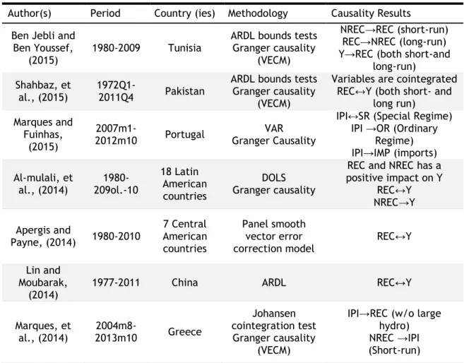
In the last few years, the literature that focused on the relationship between energy consumption and economic growth has been reoriented in order to also focus on disaggregated energy sources. This trend has inspired a lot of papers on well-established renewable energy-growth or nuclear-growth. These new approaches to the nexus generally assess the same hypothesis as the traditional approach. A summary of conclusions for both traditional and new approaches to the nexus can be found, for instance, in Omri (2014) and Ozturk (2010). Table 1 below, is a summary of recent literature, which only focuses on electricity and on separating the effects due to renewable sources from those due to non-renewable sources.

Table 1: Summary of studies on the electricity-growth nexus

Author(s) Period Country (ies) Methodology Causality Results Ben Jebli and

Ben Youssef,

(2015) 1980-2009 Tunisia

ARDL bounds tests Granger causality

(VECM)

NREC→REC (short-run) REC→NREC (long-run) Y→REC (both short-and

long-run) Shahbaz, et

al., (2015)

1972Q1-2011Q4 Pakistan

ARDL bounds tests Granger causality

(VECM)

Variables are cointegrated REC↔Y (both short- and

long run) Marques and

Fuinhas, (2015)

2007m1-2012m10 Portugal Granger Causality VAR

IPI↔SR (Special Regime) IPI →OR (Ordinary

Regime) IPI→IMP (imports) Al-mulali, et al., (2014) 209ol.-10 1980-18 Latin American countries DOLS Granger causality

REC and NREC has a positive impact on Y REC↔Y NREC→Y Apergis and Payne, (2014) 1980-2010 7 Central American countries Panel smooth vector error

correction model REC↔Y Lin and

Moubarak, (2014)

1977-2011 China ARDL REC↔Y

Marques, et al., (2014) 2013m10 2004m8- Greece Johansen cointegration test Granger causality (VECM)

IPI→REC (w/o large hydro) NREC →IPI (Short-run)

4

Y↔NREC (both short-and long-run)

Y→REC Ocal and

Aslan, (2013) 1990-2010 Turkey ARDL bounds test Toda-Yamamoto Variables are cointegrated Y→REC Pao and Fu,

(2013) 1980-2010 Brazil ECM REC↔Y

Tugcu, et al.,

(2012) 1980 -2009 G7 Hatemi-J Causality

REC≠Y (France, Italy, Canada e USA) REC↔Y (England and

Japan)) REC←Y (Germany) Yildirim, et al., (2012) 1949-2010 USA Causality of Toda-Yamamoto and Hatemi-J REC≠Y REC→Y (biomass and

waste) Apergis and Payne, (2011) 1980 - 2006 6 Central American countries Panel error

correction model REC↔Y

Apergis and Payne (2010) 1985-2005 20 OCDE countries Panel cointegration tests (Pedroni) Granger causality

REC↔Y (both short- and long-run) Apergis and Payne (2010) 1992-2007 13 Eurasian countries Error Correction Model Panel Granger causality REC↔Y Payne, (2009) 1949-2006 USA Toda-Yamamoto REC≠Y

Sari, et al., (2008)

2001m1-2005m6 USA ARDL bounds test

IPI has a positive effect in large hydro, waste, wind and fossil and a negative

one in solar

Notes: Y denotes economic growth; IPI denotes Industrial Production index; REC denotes renewable energy consumption, NREC denotes Non-renewable energy consumption, “Y↔REC” denotes Feedback hypothesis; “Y→REC” denotes Conservation Hypothesis, “Y←REC” denotes Growth Hypothesis and “Y≠REC” denotes Neutrality Hypothesis.

To the best of our knowledge, within the Iberian countries, there are very few studies focusing on the interactions between the different sources of electricity and economic activity. For Portugal, Marques and Fuinhas, (2015) found bidirectional causality between the special regime and the ordinary regime. Moreover, they found bidirectional causality between industrial production and the special regime, also revealing that economic activity drives electricity generation under the ordinary regime. However, when the special regime is divided into renewable and non-renewable sources, then the results are slightly different. Indeed, there is bidirectional causality between renewable special regime and industrial

5

production and there is unidirectional causality running from non-renewable special regime to IPI. For Spain, the analysis of the simultaneous accommodation of several sources of electricity generation, as well as the assessment of the relationships between the various sources and economic activity, remains to be carried out. Some exceptions are Ciarreta and Zarraga, (2010), who analysed the relationship between electricity consumption and economic growth from 1971 to 2005 and confirmed the growth hypothesis through both linear and non-linear Granger causality. Another exception is Fuinhas and Marques (2012) who used the ARDL bounds test approach to analyse the relationship between energy consumption and economic growth for PIGST (Portugal, Italy, Greece, Spain, and Turkey) since 1975 to 2009 and found a bidirectional causality for all countries. However, none of them analyses the idiosyncrasies of renewables and conventional sources.

Regarding the methodological pathways, much of the recent literature has aimed to assess the short- and long-run effects simultaneously. To do this, the ARDL bounds test approach has been widely used(Begum, et al., 2015; Al-mulali, et al., 2014; Ocal and Aslan, 2013). For example, the short- and long-run effects are analysed for Portugal by Shahbaz et al. (2011) using the ARDL Bounds test, UECM and VECM. They found a unidirectional causality running from economic growth to electricity consumption in the short-run and bidirectional causality in the long-run. When the short- and long-run effects were not disaggregated, bidirectional causality was found for the same country and a similar period (Tang and Tan, 2012). In general, these authors provide support for the argument that short- and long-run effects can be different. Consequently, this procedure is also followed within this study, which will more clearly assess the dynamics of interaction between electricity generation and economic activity.

2.2 Spanish Electrical system

Spain has an electricity system that is a mixture of both regulated and liberalized. Regulation is applied in accordance with "Ley 54/1997 del Sector Eléctrico” (Spain Government, 1997) . To meet the requirements of the EU (“Directiva 2009/28CE”) (European Commission, 2009) Spain created PANER (“Plan de Acción Nacinal de Energias Renobables”)(Ministerio de industria, 2010) aiming to achieve a target for renewable energy of 20% of final consumption in 2020. The consumption of electricity takes place within a liberalized market. From January of 2003, consumers were able to choose their electricity supplier. Regarding generation, it is regulated according to two regimes of electricity generation: The Special Regime and the Ordinary Regime. This system has been experiencing difficulties in accommodating generation under the special regime within the electricity system. The regulation of production under the special regime was scheduled by “Real decreto 661/2007” (Spain Government, 2007). This dual system is characterized by having a wholesale market (“Spanish Pool”). The electricity system is forced to buy the electricity produced by the Special Regime (priority order)

6

through regulated tariffs or the market. The electricity produced by the ordinary regime must be sold to the “Pool” or through bilateral contracts with consumers at market prices.

Table 2: Installed generation capacity in Peninsular Spain, by regime (MW)

2003 2005 2010 2014

Ordinary Regime 47422 54829 64813 62497 Special Regime 13801 19142 34230 39763 Total capacity 61223 73971 99043 102260

Source: Red Electrica España (El Sistema Español: 2003, 2005, 2010 and 2014).

In general, the installed capacity of electricity generation has increased. Nevertheless, we can verify that from 2003 to 2010 production under the OR first increased, but then decreased. Since 2003 to 2014, the installed capacity under the ordinary regime increased 31.789 % on average and under the special regime increased about 188.117%. During this period, the installed capacity under the OR increased, on average, 2.391% per year, while under the special regime it increased 10,098% per year. However, the installed OR capacity has decreased for the last few years, from 2010 to 2014 (see table 2).

Table 3: Evolution of installed capacity under SR (MW)

2003 2005 2010 2014

Mini-hydro 1496 1758 1991 2015

Wind 5361 9800 20057 22845

Other renewables 674 939 5190 7738

Cogeneration 6270 6445 6992 7075

Source: Red Electrica España (El Sistema Español, 2003, 2005, 2010 and 2014).

The upturn of installed capacity in the SR is well-known. When analysing every component encompassed by the SR, one can observe that the new renewables, such as wind, solar photovoltaic, thermal solar and renewable thermal have been increasing over the last eleven years. Annually, the installed capacity in wind increased 14.086% and that of other renewables increased 24.842%. Both wind and other renewables have the largest impact on the growth of installed capacity under the special regime. The non-renewable source present in the special regime (cogeneration) increased 1.104% per year in installed capacity, and mini-hydro increased 2.744% per year (see table 3).

7

3. Data and methodology

This section is dedicated to the presentation of the variables used, as well as to describe and support the methodology applied.

3.1 Data

This study uses monthly data from the January 2003 to September 2014, for the industrial production index (IPI), electricity generated from the SR and OR, imports and exports of electricity and electricity consumption for water pumping systems. All the data available until October 2014 was used. The IPI of Peninsular Spain was used to represent economic activity. It was computed by applying raw data and the corresponding weight of each

comunidad autonoma. To do this, the data was collected from the Instituto Nacional de Estadistica (INE) and the other data source is Red Eléctrica España (last update on

13/11/2014). The variables in the study are: the Ordinary Regime (OR) that includes electricity generation from large hydro, nuclear, fuel, gas and combined cycle; the Special

Regime (SR) which includes mini-hydro, wind, photovoltaic, solar thermal, renewable thermal

and thermal non-renewable; the Ratio between exports and imports (RXI) of electricity;

pumping (PUMP) which represents the electricity used in hydraulic power to raise the water

in dams for subsequent generation of electricity; and the Industrial Production Index (IPI). It is worthwhile to note that the OR not represents a non-renewable electricity sources, neither SR represents a renewable sources. However, during the period under study, the OR are mostly composed by non-renewables sources and SR is mainly composed by the renewables sources.

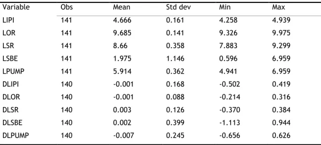
Table 4 shows the summary statistics of the variables. Thereafter, the prefixes “L” and “D” represents natural logarithm and first differences, respectively.

Table 4: Summary statistics of variables

Variable Obs Mean Std dev Min Max

LIPI 141 4.666 0.161 4.258 4.939 LOR 141 9.685 0.141 9.326 9.975 LSR 141 8.66 0.358 7.883 9.299 LSBE 141 1.975 1.146 0.596 6.959 LPUMP 141 5.914 0.362 4.941 6.959 DLIPI 140 -0.001 0.168 -0.502 0.419 DLOR 140 -0.001 0.088 -0.214 0.316 DLSR 140 0.003 0.126 -0.370 0.384 DLSBE 140 0.002 0.399 -1.113 0.944 DLPUMP 140 -0.007 0.245 -0.656 0.626

8

3.2 Methodology

At first glance, the likelihood of potential endogeneity between the variables, make it advisable to check the adequacy of using a VAR/VECM approach. However, the Vector Autoregressive model requires stationary variables. The Vector Error Correction model demands that all variables are I(1). Faced with a mixture of stationary and non-stationary variables in levels, the Toda and Yamamoto (1995) technique appears to be appropriate. Indeed, it tests similar hypothesis to that of Granger causality, but has the advantage of being able to handle series I(0), I(1) or borderline I(0)/I(1). This method also allows the capture of causalities between the variables in level with the advantage of not losing long-run effects. Once the stationary of the variables was evaluated, the Toda and Yamamoto (1995) causality test was carried out. The LM autocorrelation test, normality test (Skewness, Kurtosis and Jarque-Bera) and the White Heteroskedasticity test were performed to certify that the residuals not have serial correlation, that they are normality distributed and are homoscedastic.

In order to confirm the causalities found using the Toda-Yamamoto technique, the ARDL approach were carried out. The use of the ARDL bounds tests approach, proposed by Pesaran et al. (2001) has useful advantages. Firstly, it allows the handling of stationary and non-stationary series, provided that they are not integrated of order two. Secondly, it is more consistent in small samples than the Johansen cointegration test (Johansen and Juselius, 1990) and its conclusions are not skewed by the inclusion of dummy variables. Last but not least, it allows for handling of the potential endogeneity between variables and structural breaks that could occur in the series.

Remembering that the main objective of this work is to analyse the dynamics of interaction between proxy economic activity and the electricity generation regimes, three ARDL models were employed: Model I – economic activity; Model II – ordinary regime; and Model III –

special regime. The equations (1)-(3) represent the ARDL log-log functional specifications for Models I, II and III respectively.

, 1 5 4 3 2 1 0 t t t t t

t TREND LOR LSR LPUMP LRXI

LIPI        (1) , μ LRXI LPUMP LSR LIPI TREND LOR₀₁ _{2 t}_{3 t}_{4 t}_{5 t} _2t (2) , 3 5 4 3 2 1

0 TREND LIPIt LORt LPUMPt LRXIt t t

LSR        (3)

where, α0, φ0 and γ0 denote the intercept, μ1t, μ2t and μ3t are the stochastic disturbance terms,

assuming they are white noise and Gaussian distributed and αi, φi and γi, with i=1, …, 5,

denote the coefficients of the variables. Subsequently, these equations were converted into their ARDL equivalent general unrestricted error correction model (UECM), equations (4)-(6).

9

Model I – economic activity

, 4 1 11 1 10 1 9 1 8 1 7 0 6 0 5 0 4 0 3 1 2 1 0 t t t t t t n i i n i i n i i n i i n i i t RXI LPUMP LSR LOR LIPI DLRXI DPUMP DLSR DLOR DLIPI TREND DLIPI                                    











Model II – ordinary regime

, 5 1 11 1 10 1 9 1 8 1 7 0 6 0 5 0 4 0 3 1 2 1 0 t t t t t t n i i n i i n i i n i i n i i t LRXI LPUMP LSR LIPI LOR DLRXI DPUMP DLSR DLIPI DLOR TREND DLOR                                    











Model III – special regime

, 6 1 10 1 9 1 8 1 7 1 7 0 6 0 5 1 4 0 3 1 2 1 0 t t t t t t n i i n i i n i i n i i n i i t LRXI LPUMP LOR LIPI LSR DLRXI DPUMP DLOR DLIPI DLSR TREND DLSR                                    











where β0, θ0 and σ0 represent the intercept in models, μ4t, μ5t and μ6t are the disturbance

terms and βi, θi and σi, with i=1,…,10, represent the coefficients of the variables and in the

short-run represent the dynamics between the variables, while the coefficients of long-run multipliers of the equations and n represent the maximum order of lags that is tested.

The quality of the estimations was exhaustively tested. Accordingly, the diagnostic tests: LM autocorrelation test, ARCH heteroskdaticity test and Jarque-Bera normality test; and the stability tests: cumulative sum of recursive residuals (CUSUM), cumulative sum of squares of recursive residuals (CUSUMSQ) and RESET tests were performed. In this way, it was checked that the residuals no have serial correlation, that they are homoscedastic and normality distributed. Checks were also undertaken to show that the models were stable and correctly specified. After estimating the models, the use of the ARDL bounds test allows an examination for the presence of cointegration of the variables. The use of Toda-Yamamoto causality test follows recent literature such as Payne, (2009) and Yildirim, et al., (2012) as well as ARDL bounds test (see Ben Jebli and Ben Youssef, 2015b; Lin and Moubarak, 2014; Shahbaz, et al., 2015) and as both methods jointly (see Ocal and Aslan, 2013)

10

4. Results

This section is dedicated to showing the results. The first subsection analyses the data characteristics, while the second and third subsections are focused on the results from the Toda-Yamamoto causality and the ARDL bounds test approach, respectively.

4.1 Unit root test

The visual inspection of the series was carried out (figure 1) in the first step to assess the stationary of the series. All the series under study appears as non-stationary at their levels, once, the mean and the variance of the variables are not constant throughout the entire time span. The visual inspection of LIPI series also suggests the presence of both a structural break and a seasonal break in August.

Figure 1: Variables in levels

7.8 8.0 8.2 8.4 8.6 8.8 9.0 9.2 9.4 03 04 05 06 07 08 09 10 11 12 13 14 LSR -1.0 -0.5 0.0 0.5 1.0 1.5 2.0 03 04 05 06 07 08 09 10 11 12 13 14 LRXI 4.8 5.2 5.6 6.0 6.4 6.8 7.2 03 04 05 06 07 08 09 10 11 12 13 14 LPUMP 4.2 4.3 4.4 4.5 4.6 4.7 4.8 4.9 5.0 03 04 05 06 07 08 09 10 11 12 13 14 LIPI 9.3 9.4 9.5 9.6 9.7 9.8 9.9 10.0 03 04 05 06 07 08 09 10 11 12 13 14 LOR

11

After that, the unit root tests, Augmented Dickey-Fuller (ADF) test (Dickey and Fuller, 1981), Perron (PP) (Phillips and Perron, 1988) and Kwiatkowski Phillips Schmidt Shin (KPSS) test (Kwiatkowski, et al., 1992) were performed to assess the variables’ integration order. The ADF tests were carried out under the null hypothesis of unit root and following the Schwarz information criterion. The PP test used the same null hypothesis as the ADF test, but used the Bartlett kernel spectral estimation method and the Newey-West bandwidth. The KPSS tests had the null hypothesis of stationarity and used the Bartlett kernel spectral estimation method and the Newey-West bandwidth. Overall, the outcomes of the unit root tests (table 5) proved inconclusive about the order of integration of variables. Consequently, the Johansen and Juselius (1990) cointegration approach could not be used. Once it was confirmed that the variables were not integrated of order two I(2), the ARDL bounds test (Pesaran, et al., 2001), became more suitable for handling these database characteristics.

Table 5: Results of unit root tests

ADF PP KPSS CT C None CT C None CT C LIPI -2.2642 -0.6434 -0.9684 -11.8183*** -8.8821*** -0.2918 0.2019** 1.1948*** ∆LIPI -1.9092 -1.9832 -1.847** -32.6574*** -32.7454*** -32.8047*** 0.0415 0.0446 LOR -2.3810 0.0419 -1.0328 -6.0176*** -4.6845*** -0.3249 0.3486*** 1.055023*** ∆LOR -2.5223 -2.5595 -2.3955** -22.8742*** -22.7596*** -22.6277*** 0.10775 0.105528 LSR -5.4534*** -1.701203 4.417974 -5.4989*** -1.9241 0.5761 0.1664** 1.4484*** ∆LSR -9.0565*** -8.7827*** -15.7577*** -19.1884*** -19.0348*** -18.7249*** 0.176605** 0.187408 LRXI -5.5618*** -5.1773*** 2.4802** -5.4309*** -4.9296*** -2.8214*** 0.2634*** 0.6655** ∆LRXI -8.9744*** -8.9411*** -8.9717*** -67.6318*** -39.3472*** -37.1418*** 0.2659*** 0.3124 LPUMP -1.8081 -1.7774 -0.1488 -4.2343*** -4.2188*** -0.6015 0.1340* 0.2183 ∆LPUMP -4.8267*** -4.8503*** -4.8711*** -11.1331*** -11.1713*** -11.2146*** 0.0298 0.0296 Notes: ADF means augmented Dickey-Fuller test, PP means Phillips Perron test and KPSS means Kwiatkowski Phillips Schmidt Shin; C means constant, CT means constant and trend and None denotes without constant and trend. ***, ** and * indicate that the statistic is significant at 1%, 5% and 10%, respectively.

It is worthwhile to highlight that the results coming from the traditional unit root tests are not reliable in the presence of structural breaks, as noted by Baum (2004). The visual inspection of the series and the analysis of the correlograms and partial correlograms, both point to the likely occurrence of structural breaks in the series. To get over this limitation, Zivot and Andrews (1992) propose three models for unit root testing in the presence of structural breaks. The models allow a one-time change to be determined in a variable at a level form (model A), in a trend (model B) and in both intercept and trend (model C). This method allows us to discover if a break exists and, if so, when it occurs. It is crucial that this information is captured by an appropriate dummy variable, in order to estimate parsimonious models. The test was carried out in presence of trend and intercept both in level and in first differences with a break-point This method has also been used by Hamdi, et al., (2014) to study the electricity-growth nexus in Bahrain.

12

Table 6: Results Zivot and Andrews (1992) unit root test

T-statistic Break LIPI -7.7368*** 2008m8 DLIPI -10.4771*** 2008m8 LOR -5.3951** 2009m2 DLOR -11.5358*** 2012m12 LSR -6.3563*** 2009m10 DLSR -15.8639*** 2012m11

Notes: The critical values are 5.57 at 1%, -5.08 at 5% and -4.82 at 10%. The test was performed with trend and intercept and with maximum 4 lags; ***,**, denote significance at 1% and 5%, respectively.

The results (table 6) reveal that all series are stationary in their levels, I(0), or trend-stationary in the presence of one unknown break-point. This information about the structural breaks will be used in the subsequent estimations. Accordingly, shift dummies were used to capture the breaks occurred in the series on the first differences. Please note that this procedure occurs because in the ARDL estimations, the dependent variable are in first differences.

4.2 Toda-Yamamoto causality test

The optimal number of lags was selected following the Schwarz information criterion. It has the advantage of being a more restrictive criterion as well as coping appropriately with structural breaks. Accordingly, the optimal number is 7 and, following the Toda and Yamamoto (1995) causality test procedure, the number of lags used was 8. The shift dummies of the structural break after August 2008 and November 2012 (SD_2008m8 and SD_2012m11) were used, as well as the intercept and trend. In view of the lack of evidence for the endogeneity of the variable LPUMP, it was used as an exogenous variable.

Table 7: Diagnostic tests

Component Skewness Chi-sq kurtosis Chi-sq Jarque-Bera

LIPI -0.3803* 3.1821 3.0849 0.0066 3.2218

LOR -0.1356 0.4048 3.0707 0.0169 0.4323

LSR -0.2603 1.4905 2.4370 1.8106 3.2336

Joint 5.0775 1.8102 6.8877

Autocorrelation LM test Heteroskedasticity White test

(1)13.4422 473.5070

(2)25.9098***

(3)13.8265

Notes: Autocorrelation test refers to autocorrelation LM test; lag order is shown in (); the

13

Table 7 shows the diagnostic tests carried out on the TY causality test. These results reveal that the residuals of the model are normality distributed and do not have heteroskedastic problems. The first and third order serial correlations do not reveal autocorrelation. The autocorrelation detected for lag 2 is not a concern, given the long sample.

Table 8: Results of Toda and Yamamoto (1995) causality test

LIPI LOR LSR

LIPI does not cause - 43.4089*** 22.5423***

LOR does not cause 58.9150*** - 28.4443***

LSR does not cause 24.420*** 11.4620 -

ALL 73.2990*** 71.5507*** 58.6403***

Notes: “All” means Toda-Yamamoto causality test for all independent variables. *** denote significance at 1%.

Table 8 shows the results of the TY causality test. The feedback hypothesis is confirmed for Spain, both for the ordinary and special regime and IPI. Regarding the interaction between regimes of electricity production, it was found a unidirectional causality running from LOR to LSR. In summary, the causality relationships are LIPI↔LOR, LIPI↔LSR and LOR→LSR. It is worth noting that these results are actually in line with those from the ARDL models that it will be revealed in the next subsection.

4.3 ARDL approach

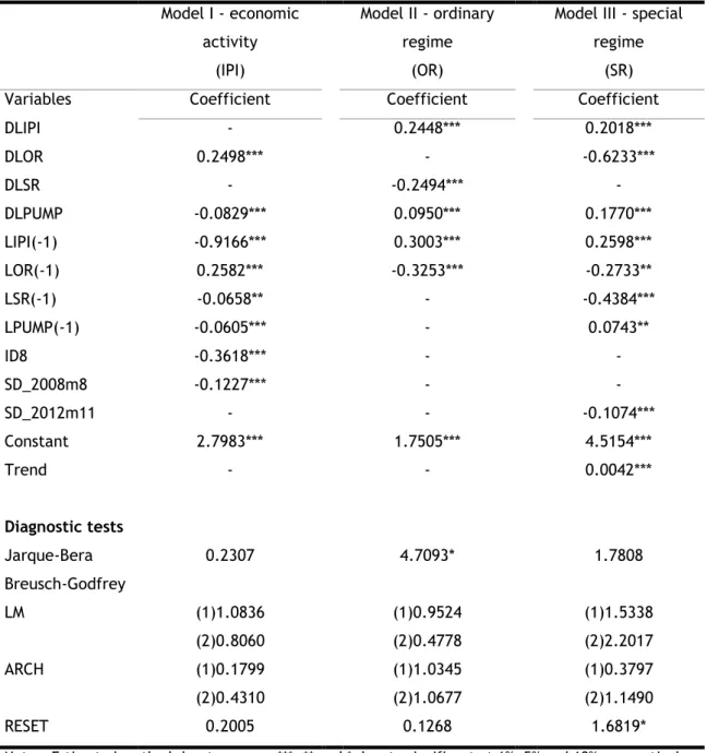
The results of the parsimonious ARDL models are shown in table 9. Once again, they are subjected to the battery of tests to assess the goodness-of-fit of the estimations, as stated above. The normality of the residuals is not rejected, with the exception of the model II-OR even if at 10% significance level. This fact is of little concern, considering that the number of observations exceeds 100. The first and second order serial correlations are not a concern for any of the models. The homoscedasticity of the residuals is confirmed by the ARCH test, and the RESET test proves the appropriate functional form of each of the models, except in the model III, even so at 10% significance level only.

14

Table 9: Results of estimated ARDL Model I - economic activity (IPI) Model II - ordinary regime (OR)

Model III - special regime

(SR) Variables Coefficient Coefficient Coefficient

DLIPI - 0.2448*** 0.2018*** DLOR 0.2498*** - -0.6233*** DLSR - -0.2494*** - DLPUMP -0.0829*** 0.0950*** 0.1770*** LIPI(-1) -0.9166*** 0.3003*** 0.2598*** LOR(-1) 0.2582*** -0.3253*** -0.2733** LSR(-1) -0.0658** - -0.4384*** LPUMP(-1) -0.0605*** - 0.0743** ID8 -0.3618*** - - SD_2008m8 -0.1227*** - - SD_2012m11 - - -0.1074*** Constant 2.7983*** 1.7505*** 4.5154*** Trend - - 0.0042*** Diagnostic tests Jarque-Bera 0.2307 4.7093* 1.7808 Breusch-Godfrey LM (1)1.0836 (1)0.9524 (1)1.5338 (2)0.8060 (2)0.4778 (2)2.2017 ARCH (1)0.1799 (1)1.0345 (1)0.3797 (2)0.4310 (2)1.0677 (2)1.1490 RESET 0.2005 0.1268 1.6819*

Notes: Estimated method: least squares. ***, ** and * denote significant at 1%, 5% and 10%, respectively. Lags of tests shown in (). RESET test means (Ramsey, 1969) and shows t-statistic, Jarque-Bera denotes normality test, Breusch-Godfrey denotes autocorrelation test and ARCH denotes heteroskedastic test.

As is well-known, industrial production suffers from a generalized downturn in the summer. A seasonality effect such as this is controlled by using a dummy variable for August (ID08). Please note that the results of the Zivot and Andrews (1992) test suggests the existence of a break beginning in August of 2008. This timing is already a milestone in Europe, first as result of the international financial crises, and then the debt crisis. Accordingly, in model I – economic activity - a shift dummy was included to handle this structural break. With regard to model II - OR, the ZA test points to a structural break beginning in December 2012. Following the procedure, the shift dummy is tested within this model. Results prove that its

15

inclusion does not bring additional explaining power to the model. In other words, the quality of the results, with or without the shift dummy, is similar. Consequently, the parsimonious model is shown and discussed. Finally, model III – SR, accommodates the break suggested by the ZA test (SD_2012m11). Please note that, the shifts dummies suggested by the ZA test in the first differences were used, because the dependent variable in the ARDL estimations are in first differences. Please note also that, the series in first differences contains as assumptions an existence of trend and constant All the dummies variables suggested by ZA and the seasonality dummy control are accommodated by the models with no problems in residuals or stability and with high significance level (1%).

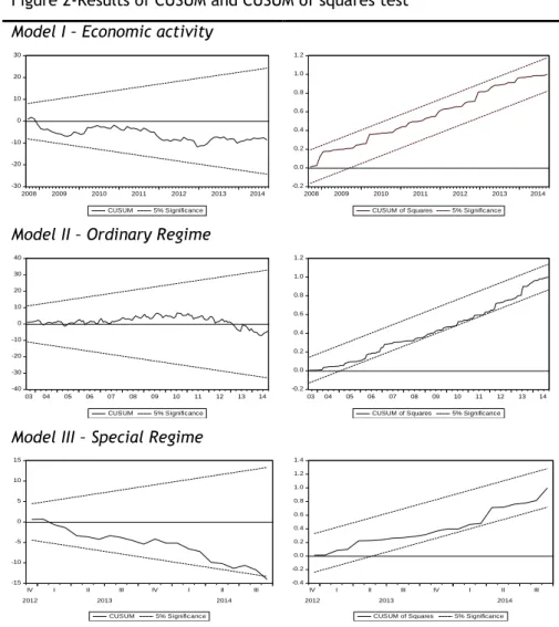
Figure 2 shows the results of both the CUSUM and the CUSUMSQ tests for the three models. On the whole, they reveal great stability in the models. Note that the period shown in figure 2 is not similar, given that dummy variables were applied in models I and III. As a consequence, the CUSUM and CUSUMSQ are computed only for the periods after the dummies’ inclusion. In turn, model II, contains no dummy variable, and as such the CUSUM and CUSUMSQ are shown for the entire period of 2003 to 2014.

Figure 2-Results of CUSUM and CUSUM of squares test

Model I – Economic activity

-30 -20 -10 0 10 20 30 2008 2009 2010 2011 2012 2013 2014 CUSUM 5% Significance -0.2 0.0 0.2 0.4 0.6 0.8 1.0 1.2 2008 2009 2010 2011 2012 2013 2014 CUSUM of Squares 5% Significance Model II – Ordinary Regime

-40 -30 -20 -10 0 10 20 30 40 03 04 05 06 07 08 09 10 11 12 13 14 CUSUM 5% Significance -0.2 0.0 0.2 0.4 0.6 0.8 1.0 1.2 03 04 05 06 07 08 09 10 11 12 13 14 CUSUM of Squares 5% Significance Model III – Special Regime

-15 -10 -5 0 5 10 15 IV I II III IV I II III 2012 2013 2014 CUSUM 5% Significance -0.4 -0.2 0.0 0.2 0.4 0.6 0.8 1.0 1.2 1.4 IV I II III IV I II III 2012 2013 2014

16

Model I - IPI shows that the LOR and LPUMP are statistically significant both in the short- and long-run. The variable LSR is statistically significant only in the long-run. This evidence proves the relationship between electricity production and economic activity. In model II - OR, the LIPI is statistically significant in both the short- and long-run. The variable LSR is not statistically significant in the long-run. This outcome allows us conclude that the system has space to accommodate more electricity generation under the SR without needing any more under the OR. Table 10 reveals the results of the Likelihood Ratio Omitted Variables test to ascertain if the LSR and LPUMP are statistically significant in the long-run on the specification of LOR. The results reveal the non-significance of LSR, LPUMP and together, thus proving that the model II-OR is not dependent on either SR or PUMP on its determination.

Table 10: Likelihood Ratio test

Model II – OR

LSR (-1) 0.9105

LPUMP (-1) 2.7325*

ALL 3.5574

Notes: * denotes significant at 10%.

Looking at model III - SR, the LOR is statistically significant in explaining the special regime. The effect is negative, which is a sign of a substitution mechanism between the regimes of electricity generation. Regarding the relationships between the two regimes and the IPI, results prove that there is a positive and significant effect of LIPI on both regimes of electricity generation.

To perform ARDL bounds test, the F-statistic is used in the Wald test, under the null hypothesis that the long-run coefficients in equations 4, 5 and 6 are equal to zero (no cointegration) and the alternative that coefficients are different from zero (cointegration). The results of the ARDL bounds tests (see table 11) reveal that, in all three models, the coefficients of the parameters are statistically different from zero. This means that all the variables are cointegrated, i.e. they have a long-run relationship.

17

Table 11: The ARDL bounds tests

Critical Values

F-statistic k Bottom Top

Model I (IPI) 120.6131*** 3 4.29 5.61

Model II (OR) 22.1641*** 1 6.84 7.84

Model III (SR) 10.3518*** 3 5.17 6.36

Notes: *** denotes significant at 1%. K is the number of independent variables. Critical values from (Pesaran, et al., 2001)

The values of the Error Correction Mechanism (ECM) are significant at 1%, and are 0.917, -0.325 and -0.438, in models I, II and III, respectively. This reveals the rapid speed of adjustment to the long-run equilibrium in model I - IPI and the moderate adjustment speeds in both models II - OR and III - SR. Bearing in mind the economic characteristics of the variables, this outcome is actually expected. Investment in electricity generation sources is not only expensive but is also a lengthy process. As such, a lower adjustment speed is anticipated.

The ARDL approach is robust in the endogeneity of variables and allows the capture of direct and indirect effects in the elasticities. Semi-elasticities (short-run) and elasticities (long-run) were performed for each model. To do this, the coefficient of explanatory variables in the long-run lagged once, was divided by the ECM coefficient, lagged once and finally multiplied by -1 (see table 12).

18

Table 12: Semi-elasticities and elasticities.

Value Model I - IPI DLOR 0.2545***

DLPUMP -0.0839*** LOR 0.2818*** LPUMP -0.0660*** LSR -0.0718** Model II - OR DLIPI 0.2427*** DLPUMP 0.0941*** DLSR -0.2430*** LIPI 0.9230*** Model III - SR DLIPI 0.2018*** DLOR -0.6233*** DLPUMP 0.1770***

LIPI 0.5927**

LOR -0.6235***

LPUMP 0.1695*** Notes: *** and **, denote significant at 1% and 5% respectively.

Results show that in the I – IPI model, a 1% increase in the long-run of the ordinary regime, the special regime and pumping system, generates a 0.282% increase, and a decrease of 0.072% and 0.066% respectively, in industrial production. In the short-run, pumping system decrease LIPI by 0.066% and electricity generation under the ordinary regime increases the LIPI by 0.254%. Regarding the II – OR model , the LIPI variable affects the OR in both the short- and long-run, while a 1% increase in LIPI in the short- and long-run generates an increase in the OR of 0.243% and 0.923%, respectively. The DLPUMP and DLSR only affect generation under the OR in the short-run by 0.094% and -0.243%, respectively. In model III, a 1% increase in the OR in both the short- and long-run, generates a decrease of 0.623% in the SR, thus reflecting the substitution effect. The LIPI in both the short- and long-run positively affects the SR by 0.202% and 0.593% respectively.

19

5. Discuss of results

Spain has been pursued its own path to meet EU targets with regard to electricity production by renewable sources. The Ordinary Regime incorporates conventional sources and large hydro. Mostly it assumes a backup role for the electricity system, thus enabling enhanced integration of the special regime. This study allowed us to more fully analyse the complexity of the relationships between these two regimes, and the relationships between them and with economic activity. This complexity is clearly visible in the differing effects that were observed in short- and long-run dynamics. The ARDL bounds test approach has proved extremely useful in this task.

The causality analysis proves that the OR is causing SR electricity generation, but the opposite is not true. Indeed, the SR is not causing the OR in Spain. Remembering that, this work is not focused in renewable and non-renewables sources, however the SR and OR represents mainly renewable and non-renewable sources, respectively. In this sense, it is comparable with studies focused on renewable and non-renewable sources, therefore our results are in line with Ben Jebli and Ben Youssef, (2015), for the Tunisia in the short-run. This achievement could not have been anticipated, given that in general, the SR requires a larger installed capacity of controllable sources as a backup for the intermittency of renewables. However, this finding is highly consistent with the results from the ARDL models. Both in the ordinary regime and special regime models, a substitution effect between these two regimes is evident. In the special regime model the substitution effect between sources is noticeable both in the short- and long-run. However, in the OR model, the Special Regime is not statistically significant on explaining the OR. Overall, these findings confirm the highly complex nature of managing an optimal generation mix, without compromising economic growth. On the other hand, additional penetration of renewables does not require additional support from fossil sources. This means that the burdens stemming from backing up renewables are substantially avoided. This fact makes deployment of the SR more attractive. However, results also support the argument that special regime are not driving economic activity. This result agrees with that of Ocal and Aslan (2013) in Turkey, and their study confirmed the conservation hypothesis, but in their ARDL the coefficients of renewable sources showed a negative signal in the long-run.

On the other hand, the whole electricity system seems to be efficient, given that it is able to release resources of one kind when it uses resources of another kind. This substitution effect is thus a clear sign of technical efficiency. Therefore, as it is not a technical matter of unrestricted electricity supply, the major challenge arising for Spanish policy-makers is economic. In other words, the negative effect observed from the SR on IPI could come from the excessive generation costs or excessive guaranteed returns from installed capacity of the

20

special regime. With regard to the OR, its effect on economic growth is positive both in the short- and long-run.

The pervading role played by pumping in the management of the transmission system operator (TSO) is entirely proven. Pumping stimulates electricity generation under both the special and the ordinary regimes. It seems that pumping is a cushion for both regimes, as was expected. Additional proof of the robustness of this empirical assessment can be observed in the difference caused by pumping in the two regimes. With regard to the OR, it is statistically significant only in the short-run. In turn, in the SR, the effect of pumping is not only of a larger magnitude in the short-run, but is also statistically significant in the long-run. This provides evidence of the crucial role of pumping in accommodating renewables within the electricity system, mainly by using excess generation from periods when substantial natural resources are available. When considering the effect of pumping on the IPI, the outcome is markedly different. Indeed, it is negative and statistically significant both in the short- and long-run, although of relatively small magnitude. This negative effect is larger in the short- than in the long-run. It is consistent not only with the well-documented high cost of pumping, but also with the specific characteristics of pumping in Spain. Indeed, according to the TSO, the source of the electricity that is used for pumping depends on the generation mix at the time of pumping and therefore varies according to when the pumping occurs. This means that this non-productive electricity consumption could use the potential of electricity generation by storing water but, at the same time, it uses electricity that could otherwise have a positive impact on the economy if it were consumed in productive activities.

It is worthwhile making two final observations. The first is to highlight that the other tool used by the TSO in managing the system, the external trade of electricity, was not shown to be significant in any model, contrary to that observed in Greece (Marques et al., 2014), and in Portugal (Marques and Fuinhas, 2015). The exiguities of the electricity market and the electrical grid’s tenuous interconnections with the rest of Europe make this tool ineffective. The second observation is to emphasize the presence of a statistically significant trend for the special regime in Spain. As is well known, EU members are committed to direct targets for the use of renewables domestically. This fact may mean that use of renewables will grow accordingly, and accomplish this increase trend, but clearly as a result of these political commitments and not due to an economic rationale to diversify the mix.

21

6. Conclusions

In this study, both the Toda-Yamamoto causality test and the ARDL bounds test approach were followed to study the dynamics of adjustment between the dual regime of generating electricity and economic activity. The focus was on continental Spain, for the time span from January 2003 to September 2014. Results prove that the short- and long-run effects are quite different. Overall, there is a strong consistency of results between the causality analyses the ARDL models.

Bidirectional causality was found between electricity consumption under both special and ordinary regime and economic activity. The causality analysis proves that the ordinary regime of electricity generation is causing the special regime, but the opposite is not true. This may signal that there is enough installed backup capacity to accommodate additional deployment of intermittent renewable sources. A substitution effect between ordinary and special regimes is detected. In the special regime model the substitution effect between sources is noticeable both in the short- and long-run. In view of the complexity of relationships detected between the two regimes and economic activity, this study also provides an extensive discussion and some recommendations towards a balanced accommodation of the dual regime within the electricity generation system in Spain.

22

7. References

Al-mulali, U., H. G. Fereidouni, and J. Y. M. Lee. 2014. "Electricity consumption from renewable and non-renewable sources and economic growth: Evidence from Latin American countries". Renewable and Sustainable Energy Reviews, 290–298.

Apergis, N., and J. E. Payne. 2010a. "Renewable energy consumption and economic growth: Evidence from a panel of OECD countries". Energy Policy, (a), 656–660.

Apergis, N., and J. E. Payne. 2010b. "Renewable energy consumption and growth in Eurasia".

Energy Economics, (b), 1392–1397.

Apergis, N., and J. E. Payne. 2011. "The renewable energy consumption-growth nexus in Central America". Applied Energy, 343–347.

Apergis, N., and J. E. Payne. 2014. "Renewable energy, output, CO2 emissions, and fossil fuel prices in Central America: Evidence from a nonlinear panel smooth transition vector error correction model". Energy Economics, 226–232.

Baum, C. F. 2004. "A review of Stata 8.1 and its time series capabilities". International

Journal of Forecasting, 151–161.

Begum, R. A., K. Sohag, S. M. S. Abdullah, and M. Jaafar. 2015. "CO2 emissions, energy consumption, economic and population growth in Malaysia". Renewable and Sustainable

Energy Reviews, 594–601.

Ben Jebli, M., and S. Ben Youssef. 2015a. "The environmental Kuznets curve, economic growth, renewable and non-renewable energy, and trade in Tunisia". Renewable and

Sustainable Energy Reviews, (a), 173–185.

Ben Jebli, M., and S. Ben Youssef. 2015b. "The environmental Kuznets curve, economic growth, renewable and non-renewable energy, and trade in Tunisia". Renewable and

Sustainable Energy Reviews, (b), 173–185.

Ciarreta, A., and A. Zarraga. 2010. "Electricity consumption and economic growth in Spain".

Applied Economics Letters, 1417–1421.

Dickey, B. Y. D. A., and W. A. Fuller. 1981. "Likelihood Ratio Statistics for Autoregressive Time Series with a Unit Root". Econometrica, 1057–1072.

European Commission. 2009. "DIRECTIVE 2009/28/EC OF THE EUROPEAN PARLIAMENT AND OF THE COUNCIL of 23 April 2009 on the promotion of the use of energy from renewable sources and amending and subsequently repealing Directives 2001/77/EC and 2003/30/EC". Official Journal of the European Communities, 16–62.

Fuinhas, J. A., and A. C. Marques. 2012. "Energy consumption and economic growth nexus in Portugal, Italy, Greece, Spain and Turkey: An ARDL bounds test approach (1965–2009)".

Energy Economics, 511–517.

Hamdi, H., R. Sbia, and M. Shahbaz. 2014. "The nexus between electricity consumption and economic growth in Bahrain". Economic Modelling, 227–237.

Johansen, S., and K. Juselius. 1990. "Maximum likelihood estimation and inference on cointegration-with applications to the demand for money". Oxford Bulletin of Economics

23

Kwiatkowski, D., P. C. B. Phillips, P. Schmidt, and Y. Shinb. 1992. "Testing the null hypothesis of stationary against the alternative of a unit root". Journal of Econometrics, 159–178. Lin, B., and M. Moubarak. 2014. "Renewable energy consumption – Economic growth nexus for

China". Renewable and Sustainable Energy Reviews, 111–117.

Marques, A. C., and J. A. Fuinhas. 2015. "The role of Portuguese electricity generation regimes and industrial production". Renewable and Sustainable Energy Reviews, 321– 330.

Marques, A. C., J. A. Fuinhas, and A. N. Menegaki. 2014. "Interactions between electricity generation sources and economic activity in Greece: A VECM approach". Applied Energy, 34–46.

Ministerio de industria, turismo y comercio. 2010. "Plan de acción nacional de energías renovables de españa (paner) 2011 - 2020".

Ocal, O., and A. Aslan. 2013. "Renewable energy consumption-economic growth nexus in Turkey". Renewable and Sustainable Energy Reviews, 494–499.

Omri, A. 2014. "An international literature survey on energy-economic growth nexus: Evidence from country-specific studies". Renewable and Sustainable Energy Reviews, 951–959. Ozturk, I. 2010. "A literature survey on energy–growth nexus". Energy Policy, 340–349.

Pao, H. T., and H. C. Fu. 2013. "Renewable energy, non-renewable energy and economic growth in Brazil". Renewable and Sustainable Energy Reviews, 381–392.

Payne, J. E. 2009. "On the dynamics of energy consumption and output in the US". Applied

Energy, 575–577.

Pesaran, M. H., Y. Shin, and R. J. Smith. 2001. "Bounds testing approaches to the analysis of level relationships". Journal of Applied Econometrics, 289–326.

Phillips, P. C. B., and P. Perron. 1988. "Testing for a unit root in time series regression".

Biometrika, 335–346.

Ramsey, J. B. 1969. "Tests for Specification Errors in Classical Linear Least-Squares Regression Analysis". Journal of the Royal Statistical Society. Series B (Methodological), 350–371.

Retrieved from

http://www.jstor.org/stable/2984219\nhttp://www.jstor.org/stable/pdfplus/2984219. pdf?acceptTC=true

Salim, R. a., K. Hassan, and S. Shafiei. 2014. "Renewable and non-renewable energy consumption and economic activities: Further evidence from OECD countries". Energy

Economics, 350–360.

Sari, R., B. T. Ewing, and U. Soytas. 2008. "The relationship between disaggregate energy consumption and industrial production in the United States: An ARDL approach". Energy

Economics, 2302–2313.

Shahbaz, M., N. Loganathan, M. Zeshan, and K. Zaman. 2015. "Does renewable energy consumption add in economic growth? An application of auto-regressive distributed lag model in Pakistan". Renewable and Sustainable Energy Reviews, 576–585.

24

Shahbaz, M., C. F. Tang, and M. Shahbaz Shabbir. 2011. "Electricity consumption and economic growth nexus in Portugal using cointegration and causality approaches".

Energy Policy, 3529–3536.

Spain Government. (n.d.). "Ley 54/1997 de 27 noviembre del sector electrico". Spain Government. 2007. "Real Decreto 661/2007, de 25 de mayo".

Tang, C. F., and E. C. Tan. 2012. "Electricity consumption and economic growth in portugal: Evidence from a multivariate framework analysis". Energy Journal, 23–48.

Toda, H. Y., and T. Yamamoto. 1995. "Statiscal inference in vector autoregressions with possibly integrated processes". Journal of Econometrics, 225–250.

Tugcu, C. T., I. Ozturk, and A. Aslan. 2012. "Renewable and non-renewable energy consumption and economic growth relationship revisited: Evidence from G7 countries".

Energy Economics, 1942–1950.

Yildirim, E., Ş. Saraç, and A. Aslan. 2012. "Energy consumption and economic growth in the USA: Evidence from renewable energy". Renewable and Sustainable Energy Reviews, 6770–6774.

Zivot, E., and D. W. K. Andrews. 1992. "Further Evidence on the Great Crash, the Oil-Price Shock, and the Unit-Root Hypothesis". Journal of Business & Economic Statistics, 251.