Luís Diogo Universidade Federal Fluminense
Instituto de Matemática e Estatística, Departamento de Matemática Aplicada R. Prof. Marcos Waldemar de Freitas Reis, s/n, Bloco G - Campus do Gragoatá São Domingos, Niterói, RJ, 24210-201, Brasil
e-mail: ldiogo@id.uff.br
Resumo: Apresentamos uma fórmula para o polinómio de Alexander
clás-sico de um nó em termos de um invariante de nós introduzido recentemente, chamado polinómio de aumentação e definido a partir da homologia de con-tacto do nó. Damos uma ideia da prova, que parte de uma definição dinâmica do polinómio de Alexander e envolve a análise de vários espaços de moduli de curvas pseudoholomorfas.
Abstract We present a formula expressing the classical Alexander
polyno-mial of a knot in terms of a very recent knot invariant, called the augmenta-tion polynomial and defined using knot contact homology. We give an idea of the proof, which starts from a dynamical definition of the Alexander poly-nomial and involves analyzing several moduli spaces of pseudoholomorphic curves.
palavras-chave: geometria simplética, curvas pseudoholomorfas,
invari-antes de nós.
keywords: symplectic geometry, pseudoholomorphic curves, knot
invari-ants.
1
Introduction
Knot theory and symplectic geometry have both seen a great development in recent years. In some instances, techniques from symplectic geometry have been successful in producing powerful new invariants of knots (like the knot Floer homology of Ozsváth–Szabó and Rasmussen [15, 16]), or in enhancing the understanding of previously known invariants (like a symplectic version of Khovanov homology [1]). In this note, we present a recent result ob-tained in collaboration with Tobias Ekholm, which yields a formula for the Alexander polynomial of a knot in terms of its augmentation polynomial. The former is a classical cornerstone of knot theory. The latter is a recently
defined object, introduced in the context of knot contact homology. This is another very powerful new invariant of knots that was constructed using tools from symplectic geometry. Our result is saying that knot contact ho-mology recovers the Alexander polynomial. Although this fact was already known from the work of Ng [14], the formula in terms of the augmentation polynomial appears to be new. It also has an unusual form for a relation between two polynomials. Our result will be stated as Theorem 5.1 below.
We will begin with a brief introduction to knots and the Alexander poly-nomial, including a dynamical definition of this invariant that will be useful for our purposes. Then, we change direction and give a quick introduction to symplectic geometry and pseudoholomorphic curves. After that, we explain how to use pseudoholomorphic curves to define knot contact homology, and how the latter yields the augmentation polynomial of a knot. Then, we state our result and give a terse presentation of the proof. Our goal will not be to convey the full logical structure of the argument (let alone its technical details), but only to give an idea of a practical and hopefully interesting ap-plication of pseudoholomorphic curves in symplectic geometry. We conclude with some directions for future work.
Acknowledgements. The author wishes to thank Jorge Milhazes de Freitas, Samuel Lopes and Diogo Oliveira e Silva, the organizers of the conference Matemáticos Portugueses pelo Mundo in 2019 in Porto, for the invitation to participate in that very intereresting event. Thanks are also due to Diogo Oliveira e Silva and the anonymous referees for many useful comments about this text.
2
Knots and the Alexander polynomial
2.1 Knots and links
A knot is a closed embedded curve in R3. This means that it is the image of a C8-smooth injective map from the circle S1 to R3, with non-zero derivative
at every point. A link is a finite collection of knots that are all pairwise disjoint. We are interested in knots and links from the point of view of topology, in the sense that we don’t want to distinguish those that differ by a smooth deformation causing no self-intersections, called an isotopy. Formally, this is a C8-smooth map f : r0, 1sˆR3
Ñ R3, such that ft– f pt, .q is a diffeomorphism of R3 for every t P r0, 1s, and f
0 is the identity. Two
links are isotopic if there is an isotopy f such that the image under f1 of
one link is the other link.
In Figure 1 we have the two simplest examples of knots: the unknot and the trefoil. We can think of this picture as the result of projecting our knots
Figure 1: The unknot and the trefoil (with three crossings)
in R3 to a plane, so that the projection is injective at all but finitely many points, called crossings. A figure like this, encoding for each crossing which of the two strands is over the other, is called a link diagram.
It is intuitively clear that the unknot and the trefoil are not isotopic, but it is not entirely obvious how to prove this fact. The main problem in knot theory is to find an efficient way of deciding when two knots are isotopic.
2.2 The Alexander polynomial
One of the first tools that were created to distinguish knots and links is the Alexander polynomial. Given a link L, its Alexander polynomial AlexLis a Laurent polynomial in one variable µ. This means that the integer powers of µ are allowed to be negative. Define AlexLas follows: pick an orientation for L, which is to say a direction for each of its component knots, and impose
• Alexunknot“ 1. • The skein relation:
Alex « ff ´ Alex « ff ` pµ1{2´ µ´1{2q Alex « ff “ 0 This is a relation between Alexander polynomials of three links with link diagrams that are equal outside the depicted neighborhood of a crossing.
• Isotopy invariance: AlexL“ AlexL1 if L and L1 are isotopic links. These three properties determine the Alexander polynomial for every link. Two non-obvious facts are that the Alexander polynomial is well-defined (in particular, the skein relation holds for every link diagram) and that it contains only integer powers of µ, even though the skein relation involves fractional powers.
As an example, let us compute the Alexander polynomial of the trefoil. Applying the skein relation, we get
Alex » — — – fi ffi ffi fl“ Alex » — — – fi ffi ffi fl´ pµ 1{2 ´ µ´1{2q Alex » — — – fi ffi ffi fl “ 1 ´ pµ1{2´ µ´1{2q Alex » — — – fi ffi ffi fl
where we used the fact that Alexunknot “ 1. The link we obtained on the right is called Hopf link. Let us apply the skein relation on a crossing of this link: Alex » — — – fi ffi ffi fl“ Alex » — — – fi ffi ffi fl´ pµ 1{2 ´ µ´1{2q Alex » — — – fi ffi ffi fl “ Alex » — — – fi ffi ffi fl´ µ 1{2 ` µ´1{2
where we used again that Alexunknot“ 1. To finish the computation, we need to determine the Alexander polynomial of the link with two components on the right. Since the two components can be moved by an isotopy to lie in two disjoint open balls, the link is said to be trivial. We call it the unlink with two components. Its Alexander polynomial is zero, and we leave the proof of that to the reader as an exercise on the skein relation. We can now conclude the calculation of the Alexander polynomial of the trefoil:
Alextrefoil“ 1 ´ pµ1{2´ µ´1{2qp0 ´ µ1{2` µ´1{2q “ µ ´ 1 ` µ´1.
Since this is different from the Alexander polynomial of the unknot, we can conclude that the unknot and the trefoil are not isotopic.
Exercise 1. Compute the Alexander polynomial of the figure-eight knot (the closure of the sailor’s knot of the same name), depicted in Figure 2.
2.3 A dynamical definition of the Alexander polynomial
The definition of Alexander polynomial of a link that we gave in the previous section is very suitable for computations (at least for link diagrams without
Figure 2: The figure-eight knot
too many crossings). Nevertheless, it is only one of many definitions of this invariant. We now present a different definition of the Alexander polynomial of a link, with a very different flavour. For simplicity, we will restrict our attention to the particular class of fibered knots, which we now define.
In this section, it will be convenient to think of the ambient space of a knot as the sphere S3, instead of R3. This is reasonable, since we can identify R3 with the complement of a point in S3. For this identification, two knots are isotopic in R3 if and only if they are isotopic in S3.
We say that a knot K is fibered if there is a C8-smooth map g : S3
zK Ñ S1 with no critical points. This means that the knot complement S3zK is a fiber bundle over S1, with fiber a surface whose boundary is K (such
a surface is called a Seifert surface). The differential of the function g is a 1-form dg. If we choose some Riemannian metric x., .y on S3, then the function g also specifies a vector field in S3zK, called gradient vector field
and denoted ∇g, as follows: for every vector field v on S3zK,
x∇g, vy “ dgpvq.
Since the function g has no critical points, the vector field ∇g has no zeros. A gradient flow loop is a path γ : r0, Rs Ñ S3zK, for some R ą 0, such that
• γpRq “ γp0q (which means that γ closes up to a loop) and
• dtd`γptq˘ “ p∇gqγptq for every t P r0, Rs (that is, the time-derivative of γ coincides with ∇g at every point in γ).
Observe that if γ : r0, Rs Ñ S3zK is a gradient flow loop, then so is any multiple cover γm: r0, mRs Ñ S3zK, where m is a positive integer. Here,
γmptq “ γpt1q for t1P r0, Rs such that t1 ” t mod R. We say that a flow loop
is simple if it is not multiply covered. Given a flow loop γ, we denote by mpγq its multiplicity with respect to its underlying simple loop. For every knot K, the homology group H1pS3zK; Zq is isomorphic to Z. If we pick a generator e for this homology group, then we can associate to a flow loop γ its degree dpγq, such that the class of γ on homology is dpγqe. Note that
mpγq divides dpγq. To avoid flow loops too close to K, we will require the map g to “grow near K”.
Theorem 2.1 (Milnor [13]). The Alexander polynomial of a fibered knot K
is given by AlexKpµq “ p1 ´ µq exp ˜ ÿ γ σpγq mpγqµ dpγq ¸ (1) where the sum is over all gradient flow loops (not only the simple ones). In the formula, σpγq P t˘1u is a sign (associated to the linearized return map of γ).
This formula was generalized for all knots K by Hutchings and Lee [11]. Example 2.2. Let us see how to recover the Alexander polynomial of the unknot from formula (1). The complement of the unknot in S3 is diffeo-morphic to S1ˆ R2 (if this is not clear, try to identify both spaces with the complement of the vertical axis in R3). In coordinates pθ, x, yq for S1ˆ R2, take gpθ, x, yq “ θ ` x2` y2. For the standard product metric on S1ˆ R2, the only periodic orbits are the covers of the central circle S1ˆ t0u, and all the signs σpγq in (1) are positive. The sum over flow loops becomes
ÿ ką0 1 kµ k “ ´ lnp1 ´ µq hence
Alexunknotpµq “ p1 ´ µq exp p´ lnp1 ´ µqq “ 1 as we already knew.
3
Some symplectic geometry
3.1 Classical mechanics and symplectic geometry
Symplectic geometry is a recent area of mathematics, with its roots in classi-cal mechanics, but with deep connections to other areas of mathematics and physics. In the Hamiltonian formulation of classical mechanics, a particle moving in R3 is described by its trajectory in the phase space R6, which keeps track of the position and momentum of the particle. If we denote position variables in R3 by q1, q2, q3 and the corresponding momentum
vari-ables by p1, p2, p3, then the trajectory of the particle in phase space satisfies
Hamilton’s equations # 9 qi “ BpiH 9 pi “ ´BqiH
where the Hamiltonian function H : R6 Ñ R is the energy of the particle. This trajectory is a flow line of the Hamiltonian vector field, which we denote by XH. If we define a differential 2-form on R6 by
ω –
3
ÿ
i“1
dpi^ dqi, (2)
then Hamilton’s equations above tell us that the vector field XH is given by the condition
ωp., XHq “ dH. (3)
A reader unfamiliar with differential forms may find it mildly useful to think of ω as a way of prescribing signed areas to 2-dimensional oriented surfaces in R6 (where the signs depend on the orientations of the surfaces).
We can interpret equation (3) as saying that the 2-form ω allows us to do Hamiltonian mechanics for any function that we choose to call energy on R6. We can think of symplectic geometry as generalizing this point of view on mechanics to any differentiable manifold of even dimension 2n, equipped with a differential 2-form ω whose properties mimic those of the form (2), namely:
• ω is closed: dω “ 0, and
• ω is non-degenerate: the n-fold wedge product ω ^ . . . ^ ω is a volume form (which means that it vanishes nowhere).
For the application to knot theory that we present in this text, it will mostly suffice to think of the symplectic manifold R6. We refer to the article by Ana Cannas da Silva in this volume [4] for more on symplectic geometry.
3.2 Pseudoholomorphic curves
In 1985, Gromov introduced the notion of pseudoholomorphic curve [10], which was revolutionary in symplectic geometry. It gave a powerful tool to study symplectic manifolds, and eventually led to many deep relations to algebraic geometry and theoretical physics, in particular the so called mirror symmetry phenomenon (see Lino Amorim’s article in this volume [3] for some background on mirror symmetry). Before we state one of the striking results in Gromov’s paper, let us introduce some more terminology. First, we observe that an open subset of a symplectic manifold, equipped with the restriction of the symplectic form ω, is also a symplectic manifold. Let B2nprq Ă R2n denote the open ball of radius r and centered at the
origin. Consider also the open subset B2pRq ˆ R2n´2 Ă R2n, where it is crucial that B2pRq has coordinates pp1, q1q (instead of pp1, p2q or pq1, q2q,
for instance) and R2n´2 has the remaining coordinates p2, . . . , pn, q2, . . . , qn.
Given two symplectic manifolds pM1, ω1q and pM2, ω2q, a smooth embedding
ϕ : M1 ãÑ M2 such that ϕ˚ω2 “ ω1 is called a symplectic embedding (here,
ϕ˚ is pullback by ϕ).
Theorem 3.1 (Gromov’s non-squeezing). If we have a symplectic embedding
B2nprq ãÑ B2pRq ˆ R2n´2, then r ď R.
Observe that a symplectic embedding is, by definition, volume-preserving. We can interpret Gromov’s non-squeezing as saying that not all volume-preserving embeddings are symplectic.
Now that we have given a little indication of what pseudoholomorphic curves can achieve, let us define them. We need the auxiliary notion of an almost complex structure on an even-dimensional manifold M2n, which is an endomorphism of the tangent bundle J : T M Ñ T M (covering the identity map M Ñ M ) such that J2 “ ´Id. Given such a J and a Riemann surface pS, jq, a pseudoholomorphic curve is a map u : S Ñ M satisfying the Cauchy–Riemann equation
du ˝ j “ J ˝ du.
If M has a symplectic form ω, then one can ask that ωp., J.q be a Rieman-nian metric on M , in which case J is said to be compatible with ω. Gromov’s idea was to study pM, ωq by analyzing moduli spaces of pseudoholomorphic curves (modulo domain reparametrizations, and possibly with additional structures like fixing the homology class of the map, or equipping the do-main with marked points). If J is compatible with ω, then we can control the L2-norm of u (the energy) by its ω-area, which is crucial for obtaining compactness of moduli spaces. Gromov also observed that the space of ω-compatible J is contractible, which implies that the moduli spaces defined for two different J are cobordant (that is, there is a manifold whose oriented boundary is the difference of the two moduli spaces). This allows for the definition of numerical invariants counting pseudoholomorphic curves (with appropriately chosen constraints) that depend on ω but not on the choice of ω-compatible J . Those are called Gromov–Witten invariants, and they have many applications in symplectic and algebraic geometry.
4
Symplectic knot invariants
4.1 From knots to Lagrangians and Legendrians
Recent decades have seen many applications of pseudoholomorphic curves. We will focus on a particular application to knot theory, called knot contact homology. This is part of a broader packaging of pseudoholomorphic curve information that goes by the name of symplectic field theory [8], but we will focus on the specific case of interest to us. Let us begin with some geometric constructions.
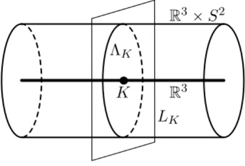
Given a knot K Ă R3 , we can define its conormal Lagrangian LK – tpq, pq P R6| q P K and p@v P TqKq xp, vy “ 0u,
where x., .y is the Euclidean inner product in R3. This is a submanifold of R6 that is diffeomorphic to S1 ˆ R2, and whose intersection with R3q
(the subspace of R6 where all pi “ 0) is the knot K. See Figure 3 for a
geometric depiction that would greatly benefit from additional dimensions. Furthermore, LK is Lagrangian, in the sense that it has half the dimension
of the ambient space R6, and the restriction of the symplectic form ω in (2) to LK vanishes. In addition, the Lagrangian LK is exact, which means the following. The symplectic form ω in R6 has a primitive λ “ř3i“1pidqi and
the restriction λ|L admits a primitive f P C8pLq (in this case, we can take
f to be any constant function). Other exact Lagrangians are R3q and R3p.
We can identify R6 with the tangent bundle1 of R3q and, with respect to the Euclidean inner product in R3, we can identify R3ˆ S2 Ă R6 with the unit tangent bundle of R3q. Recall that the geodesic flow on the unit tangent
bundle of a Riemannian manifold Q takes a point q P Q and a unit vector v P TqQ and follows the geodesic starting at q in the direction prescribed
by v. This is an example of what is called a Reeb flow in contact geometry (hence the name “knot contact homology”), but we will not go further in that direction in this note. The conormal Lagrangian LKintersects R3ˆS2in a
2-torus ΛK, which we call conormal Legendrian (again borrowing terminology from contact geometry).
It will be useful to observe that H2pR3ˆ S2, ΛK; Zq is isomorphic to Z3.
We will explain this point, but a reader less familiar with homology groups might want to skip the details. Let us just mention that this is the reason why the augmentation polynomial below will have three variables.
1From the point of view of symplectic geometry, it would be preferable to think of the
K R3 ΛK
LK
R3ˆ S2
Figure 3: The Lagrangian LK in R6
In this paragraph, consider all homology groups with Z coefficients. The long exact sequence of the pair pR3ˆ S2, ΛKq includes the segment
H2pΛKq Ñ H2pR3ˆ S2q Ñ H2pR3ˆ S2, ΛKq Ñ H1pΛKq Ñ 0.
The first map turns out to vanish. Since H2pR3ˆ S2q – H2pS2q – Z and
H1pΛKq – Z2 (ΛK is a 2-torus), the sequence splits and we get the desired
isomorphism with Z3. We get generators for this group from the choice of a generator t for H2pS2q and of generators x, p for H1pΛKq (and a choice
of splitting). It is customary to let x be a longitude curve (projecting to K under the restriction to ΛK of the projection R3 ˆ S2 Ñ R3), and to let p
be a meridian curve (mapping to a constant under that same projection). Note that such a meridian curve p lies in a cotangent fiber (that is, a 3-dimensional subspace of R6 with constant qi variables), hence the use of the
letter associated with momentum.
4.2 Knot contact homology
We can now use pseudoholomorphic curves to associate a chain complex to the knot K. We will actually get a differential graded algebra (dga), which is a chain complex with a product satisfying the (graded) Leibniz rule. Our chain complex will be a tensor algebra generated by geodesic chords starting and ending in ΛK. By this we mean paths c : ra, bs Ñ R3ˆS2 that follow the
geodesic flow and for which cpaq and cpbq P ΛK. We don’t want to get into
details, but these chords are graded by a Maslov index (which is an integer). Let us specify the ring over which we take the tensor algebra. This will be group ring (over C) of H2pR3 ˆ S2, ΛK; Zq, which, in light of the
discussion at the end of the previous section, can be identified with the Laurent polynomial ring R “ Crλ˘1, µ˘1, Q˘1s, under the identifications
The differential in the chain complex counts pseudoholomorphic curves in RˆpR3ˆS2q “ R4ˆS2(which we can identify with the complement of R3q
in R6), as follows. We define the differential for geodesic chords, and extend by linearity and the Leibniz rule. The differential of a geodesic chord x is
Bx “ ÿ y1,...,yk ¨ ˝ ÿ uPMpx;y1,...,ykq rpuq ˛ ‚y1b . . . b yk
where the first sum is over finite sequences of geodesic chords and the second sum is over elements of the moduli space of pseudoholomorphic curves u in R4ˆ S2, whose domain is a disk with k ` 1 punctures on the boundary. The boundary components map to R ˆ ΛK. At the boundary punctures, u is
asymptotic to the fixed geodesic chords, with x at `8 and the yi at ´8
(both infinities in the first R summand of the target R ˆ pR3 ˆ S2q). See Figure 4 for an illustration of one such u. Finally, the coefficient rpuq P R keeps track of the relative homology class of u in H2pR3ˆ S2, ΛK; Zq. We
will not go into more details at this point, but the reader may have noticed that more choices are necessary, including of “capping half-disks” for the geodesic chords (to obtain a relative homology class).
u P Mpx; y1, y2q x R ˆ ΛK R ˆ pR3ˆ S2q ΛK y1 y2 Figure 4: A contribution to Bx
Theorem 4.1 (Ekholm–Etnyre–Ng–Sullivan [6]). The differential B defined
above squares to zero. The homology of this dga is an invariant of the knot. This homology is called knot contact homology. It is sometimes useful to keep track of the dga, denoted by AK, instead of passing to homology.
Although the technical details of the proof of Theorem 4.1 are quite in-volved, the idea is by now standard in symplectic geometry. To prove an
algebraic identity like B2 “ 0, one interprets the contributions to B2 as ele-ments in the boundary of a suitably defined moduli space of pseudoholomor-phic curves. By showing that this moduli space is a compact 1-dimensional oriented manifold, one concludes that the signed count of the elements in its boundary is zero.
Knot contact homology appears to be a strong knot invariant, but it is not yet clear just how strong. A recent result shows that a small but non-trivial enhancement of knot contact homology is a complete knot invariant (that is, two knots are isotopic if and only if their enhanced knot contact homologies are isomorphic) [7].
4.3 Augmentations
Although the definition of the dga AK involves pseudoholomorphic curves, which can be very difficult to analyze, the dga turns out to admit a combina-torial model, which can be written down explicitly given a braid presentation for the knot K [6]. Nevertheless, since the chain complex (a tensor algebra) is very large, it can be difficult to extract useful information from its homol-ogy. One way of obtining more treatable information about the dga is via its augmentations. An augmentation is a unital dga map
ε : AK Ñ C,
where the field C is thought of as a dga supported in degree zero and with trivial differential. In other words, ε is a graded unital ring map (so, it is only non-trivial on the degree zero part of AK) satisfying ε ˝ B “ 0.
Example 4.2. One important source of augmentations is given by exact La-grangians in R6 “which look like ΛK near infinity” (in some precise sense). A key example is the conormal LK. Given such a Lagrangian, we can define an augmentation by assigning to each geodesic chord of degree 0 the count of pseudoholomorphic disks in R6 with boundary on the Lagrangian and one puncture on the boundary, where the disk is asymptotic to the geodesic chord “at infinity”. The value of the augmentation on the coefficient ring R is constrained by the topology of the Lagrangian and its ambient space. In the case of LK, since the meridian p-curve is contractible in LK and the t-sphere is null-homologous in R6, it turns out that µ “ 1 “ Q, but λ is not constrained. So, for each value λ P Czt0u we get an augmentation of AK.
It turns out to be useful to also think of the space of augmentations geometrically. We define the augmentation variety of K, denoted by VK, to consist of the union of maximal dimensional components of the Zariski closure of the set
tpεpλq, εpµq, εpQqq P pCzt0uq3| ε is an augmentationu.
The existence of the augmentations associated to LK in Example 4.2 im-plies that, for every knot K, the augmentation variety VK contains the line tpλ, 1, 1qu (where λ can be any element in Czt0u).
Theorem 4.3 (Diogo–Ekholm [5]). For every knot K, the augmentation
variety VKis an affine algebraic subvariety of pCzt0uq3of complex dimension
at least 2.
Conjecturally, VK is always 2-dimensional (so it is not all of pCzt0uq3).
Define the augmentation polynomial of K (denoted by AugKpλ, µ, Qq) as a polynomial with no repeated factors that generates the vanishing ideal of this variety: VK “ V pAugKq.
Example 4.4. The augmentation polynomial of the unknot is AugU “ 1 ´ λ ´ µ ` λµQ
and that of the trefoil is
AugT “ λ2pµ´1q`λpµ4´µ3Q`2µ2Q2´2µ2Q´µQ2`Q2q`pµ3Q4´µ4Q3q. The augmentation polynomial has deep and surprising connections to string theory and to other knot invariants. It is conjecturally the same as the so-called Q-deformed A-polynomial, which is relevant for mirror symmetry and is related in a deep way with another important knot invariant called the colored HOMFLYPT polynomial [2, 9].
5
The Alexander polynomial from the
augmenta-tion polynomial
As we have seen, the Alexander polynomial and the augmentation polyno-mial are knot invariants defined in very different ways. Nevertheless, they are related in the following surprising manner.
Theorem 5.1 (Diogo–Ekholm [5]). Recall that λ “ ex, µ “ ep and Q “ et. We have AlexKpµq “ p1 ´ µq exp ˜ ż ´BQAugK BλAugK ˇ ˇ ˇ ˇ pλ,Qq“p1,1q dp ¸ (4)
In formula (4), the integral symbol represents an antiderivative. We will give a brief idea of why one might expect the formula to hold, at least for fibered knots. We will be very imprecise and will not justify most of our claims. Our goal is to illustrate how the study of moduli spaces of pseu-doholomorphic curves can lead to meaningful algebraic identities (we already saw that this is also the idea of the proof that B2“ 0 in the dga A
K). Note
that, according to Milnor’s formula (1), we only need to argue that d dp ¨ ˝ ÿ γ in S3zK σpγq mpγqµ dpγq ˛ ‚“ ´ BQAugK BλAugK ˇ ˇ ˇ ˇ pλ,Qq“p1,1q . (5)
Exercise 2. Apply formula (4) to Example 4.4 to recover the Alexander polynomials of the unknot and the trefoil. The Alexander polynomial is often defined up to a power of µ, and (4) should also be allowed that ambiguity.
5.1 From flow loops to pseudoholomorphic annuli
The left side of (5) involves orbits in S3zK, whereas the right side involves pseudoholomorphic curves in R4 ˆ S2. To get a reformulation of the left side also in terms of pseudoholomorphic curves, we need another geometric ingredient. Recall that the conormal Lagrangian LK Ă R6 intersects R3q in the knot K. There is a procedure called Lagrangian surgery, which produces another Lagrangian submanifold by smoothing out the union of LK with R3q
(the version we need is described in [12]). Denote the new Lagrangian in R6 by MK. This submanifold is diffeomorphic to R3zK. Since LK and R3q
are exact Lagrangians, one can ensure that MK is also exact. In particular,
it has an associated family of augmentations εMK, sending both generators λ and Q of the coefficient ring R to 1, and the generator µ to any element of Czt0u. Hence, the line tp1, µ, 1qu is also contained in the augmentation variety VK for every K. The key role of these augmentations is the reason behind taking λ “ Q “ 1 in formula (4).
In R6, we can consider pseudoholomorphic annuli between R3q and MK.
These are pseudoholomorphic maps u : S1ˆ r0, As Ñ R6 (for some A ě 0) such that the restriction of u to S1ˆ t0u maps to R3q and the restriction to S1ˆ tAu maps to MK. Denote the moduli space of such pseudoholomorphic
annuli by MpR3q; MKq.
The following result is stated in an overly simplified and somewhat im-precise manner.
Proposition 5.2. For suitable choices of g : S3zK Ñ S1, metric on S3 and
pseudoholomor-MK y z1 MK z2 R ˆ ΛK
Figure 5: Definition of F pλ, µ, Qq. The curve at the top could have arbi-trarily many negative punctures capped by disks with boundary in MK.
phic annuli in MpR3q; MKq. Therefore, the sum on the left side of (5) can
be rewritten as Apµq – ÿ uPMpR3 q;MKq σpuq mpuqµ dpuq (6)
for suitable signs σpuq and integers mpuq and dpuq. Equation (5) is thus equivalent to
d dppApµqq “ ´ BQAugK BλAugK ˇ ˇ ˇ ˇ pλ,Qq“p1,1q , (7)
where we recall again that µ “ ep.
5.2 From pseudoholomorphic annuli to knot contact homology
Instead of showing equation (7) directly, we show that d dppApµqq “ ´ BQF BλF ˇ ˇ ˇ ˇ pλ,Qq“p1,1q , (8)
for a suitable holomophic function F pλ, µ, Qq such that BQF BλF ˇ ˇ ˇ ˇ pλ,Qq“p1,1q “ BQAugK BλAugK ˇ ˇ ˇ ˇ pλ,Qq“p1,1q . (9)
The function F is defined as follows. For an appropriately chosen gen-erator y of degree 1 of the dga AK (actually, an R-linear combination of such generators), take its dga differential B, which is an expression in λ, µ, Q and other generators z1, . . . , zn. Then, send the zi to their images under
the augmentation εMK. See Figure 5.
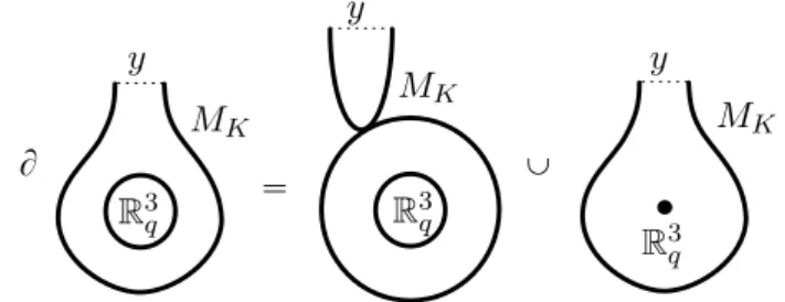
Now, consider the moduli space of pseudoholomorphic annuli in R6, with
y y y MK R3q R3q R3q MK MK B “ Y
Figure 6: The boundary of a 1-dimensional moduli space
above), but with a puncture on the boundary component mapping to MK.
At this puncture, the curve is asymptotic to y. See the left side of Figure 6. This moduli space is compact and 1-dimensional (since y has degree 1) and (if y is chosen carefully) its boundary has components of two types, which are depicted on the center and right in Figure 6. In the center con-figuration, the curve develops a node and breaks into a pseudoholomorphic plane asymptotic to y and an annulus in MpR3q; MKq. The boundaries of the
plane and annulus intersect. In the rightmost configuration, the boundary loop in R3
q shrinks to a point, so the punctured annulus becomes a plane.
A further study of the pseudoholomorphic planes in the center configu-ration reveals that the count of such broken curves (using µ to keep track of the homology of boundaries mapping to MK) is given by
dA dp . BF Bx ˇ ˇ ˇ ˇ pλ,Qq“p1,1q “ dA dp . BF Bλ ˇ ˇ ˇ ˇ pλ,Qq“p1,1q ,
recalling once more that λ “ ex. The derivatives in the formula keep track of the intersection of the boundaries of the disk and annulus. Similarly, the counts of curves in the configuration on the right turn out to be encoded by
BF Bt ˇ ˇ ˇ ˇ pλ,Qq“p1,1q “ BF BQ ˇ ˇ ˇ ˇ pλ,Qq“p1,1q ,
where Q “ et. This time, the derivative keeps track of the fact that the disk intersects R3q. Since these two configurations are the boundaries of
a compact 1-dimensional manifold, the sum of their contributions (with appropriate signs) vanishes. This implies that
dA dp . BF Bλ ˇ ˇ ˇ ˇ pλ,Qq“p1,1q `BF BQ ˇ ˇ ˇ ˇ pλ,Qq“p1,1q “ 0, which gives equation (8), as wanted.
For a brief justification of equation (9), let us just say that one can argue that F vanishes on the augmentation variety VK, so it should be of the form
F “ g AugK
for some analytic function gpλ, µ, Qq. Equation (9) now follows from the product rule for derivatives and the fact that AugK vanishes along the line tp1, µ, 1qu Ă VK (at least if we assume that g|pλ,Qq“p1,1q is not identically
zero, which as it turns out we can).
5.3 Outlook
Theorem 5.1 should not be thought of as an efficient way of computing the Alexander polynomial of a knot, but rather as an unexpected relation between two very different knot invariants. It also suggests further investi-gation in a few directions. For example, one might not set Q “ 1 in equation (4) and get a Q-deformed version of AlexK.
Question 5.3. What is the significance of this deformation of the Alexander
polynomial? Is it related to other deformations, coming for instance from knot Floer homology [15]?
One might also wonder about the condition of non-vanishing of the de-nominator in the theorem. As it turns out, this condition cannot be ne-glected, as it does not hold, for instance, for the 820 knot (as pointed out to us by Lenny Ng).
Question 5.4. Is there an analogue of equation (4) when the denominator
in the formula vanishes?
It is likely that along some branch of the variety VK, corresponding to the augmentation MK, one could find such an analogue.
As a final note, the reader may have wondered about interpreting the integrand in formula (4) via implicit differentiation. Indeed, since VK is the vanishing locus of AugK, that integrand is the partial derivative BQBλ along the line tp1, µ, 1qu Ă VK. This leads to an alternative interpretation of the
right side in the formula, related to curve counts in the resolved conifold (the total space of the bundle OCP1p´1q ‘ O
CP1p´1q), in the spirit of [2].
That is another interesting story, but unfortunately it is beyond the scope of this discussion.
References
[1] M. Abouzaid and I. Smith, “Khovanov homology from Floer cohomology”,
Journal of the American Mathematical Society, Vol. 32 (2019), pp. 1–79.
[2] M. Aganagic, T. Ekholm, L. Ng and C. Vafa, “Topological strings, D-model, and knot contact homology”, Advances in Theoretical and
Mathemat-ical Physics, Vol. 18, No. 4 (2014), pp. 827–956.
[3] L. Amorim, “Open and closed mirror symmetry”, Boletim da Sociedade
Por-tuguesa de Matemática, N. 77 (2019), pp. 15–26.
[4] A. Cannas da Silva, “An invitation to symplectic toric manifolds”, Boletim da
Sociedade Portuguesa de Matemática, N. 77 (2019), pp. 119–132.
[5] L. Diogo, T. Ekholm, “Augmentations, annuli, and Alexander polynomials”, in preparation.
[6] T. Ekholm, J. Etnyre, L. Ng and M. Sullivan, “Knot contact homology”,
Geometry & Topology, Vol. 17, No. 2 (2013), pp. 975–1112.
[7] T. Ekholm, L. Ng and V. Shende, “A complete knot invariant from contact homology”, Inventiones mathematicae, Vol. 211, No. 3 (2018), pp. 1149–1200. [8] Y. Eliashberg, A. Givental and H. Hofer, “Introduction to symplectic field theory”, Geometric and Functional Analysis Special Volume, Part II, 2000, pp. 560–673.
[9] S. Garoufalidis, A. Lauda and T. Lê, “The colored HOMFLYPT function is q-holonomic”, Duke Mathematical Journal, Vol. 167, No. 3 (2016), pp. 397–447. [10] M. Gromov, “Pseudo holomorphic curves in symplectic manifolds”,
Inven-tiones mathematicae, Vol. 82, No. 2 (1985), pp. 307–347.
[11] M. Hutchings and Y.-J. Lee, “Circle-valued Morse theory and Reidemeister torsion”, Geometry & Topology, Vol. 3 (1999), pp. 369–396.
[12] C. Y. Mak and W. Wu, “Dehn twist exact sequences through Lagrangian cobordism”, Compositio Mathematica, Vol. 154, No. 12 (2018), pp. 2485–2533. [13] J. Milnor, “A duality theorem for Reidemeister torsion”, Annals of
Mathemat-ics, Vol. 76, No. 2 (1962), pp. 137–147.
[14] L. Ng, “Framed knot contact homology”, Duke Mathematical Journal, Vol. 141, No. 2 (2008), pp. 365–406.
[15] P. Ozsváth and Z. Szabó, “Holomorphic disks and knot invariants”, Advances
in Mathematics, Vol. 186, No. 1 (2004), pp. 58–116.
[16] J. Rasmussen, “Floer homology and knot complements”, PhD thesis, Harvard University, USA, 2003.